RESEARCH ARTICLE
A graph optimization approach
for motion estimation using inertial
measurement unit data
Kiyoshi Irie
*Abstract
This study presents a novel approach for processing motion data from a six-degree-of-freedom inertial measurement unit (IMU). Trajectory estimation through double integration of acceleration measurements results in the generation and accumulation of multiple errors. Existing IMU-based measurement methods often use constrained initial and final states to resolve these errors. The constraints on the initial and final states lead to a uniform distribution of the accumulated errors throughout the calculated trajectory so that they cancel each other. We develop a generalized method that can incorporate the constraints from the measurements of intermediate states. The proposed approach is inspired by graph-based simultaneous localization and mapping processes from robotics research. We tested the proposed method with simulated and actual IMU data and found that our method estimates trajectories more accu-rately than conventional methods with acceptably higher computational costs.
Keywords: Motion estimation, Inertial measurement unit, Graph-based simultaneous localization and mapping
© The Author(s) 2018. This article is distributed under the terms of the Creative Commons Attribution 4.0 International License (http://creat iveco mmons .org/licen ses/by/4.0/), which permits unrestricted use, distribution, and reproduction in any medium, provided you give appropriate credit to the original author(s) and the source, provide a link to the Creative Commons license, and indicate if changes were made.
Introduction
Background
Measuring athlete motion is an important aspect of sports science. The typical instruments employed for this purpose include high-speed video cameras and infrared motion capture cameras. However, these instruments are expensive and require time and effort for installation.
Recently, small and inexpensive inertial measurement units (IMUs) have become available, making sports motion measurements accessible to a wide range of people. For example, measurement devices that can be attached to a golf club [1, 2] or a tennis racket [3] have been developed.
Considering these applications, this study seeks to improve the data-processing algorithm for extracting trajectories from IMU data. The IMU employed herein is assumed to comprise a three-axis accelerometer and a three-axis gyroscope. We aim to estimate a time series
of the attitude, velocity, and position values with a time series of acceleration and angular velocity measurements.
Main issues to be addressed
The integration of IMU measurements is the simplest way to extract a trajectory from IMU data. Theoreti-cally, attitude can be calculated by integrating the angu-lar velocity, velocity can be calculated by integrating the acceleration, and position can be calculated by the double integration of the acceleration. However, position estima-tion by simple double integraestima-tion amplifies the error [4]. Even a small error in the integration of the acceleration can lead to a bias drift in the velocity values. Additionally, the integration of biased velocity causes rapid generation of the positional errors. In addition, if the measurement is performed for a long period, the attitude and velocity estimations are affected by the bias drift in the angular velocity and acceleration values. Thus, it is necessary to correct the accumulated errors.
Open Access
*Correspondence: [email protected]
Related work
Human gait analysis is a well-studied topic in IMU-based motion estimation. Several methods that can precisely track human gait have been developed [5, 6]. Error cor-rection methods for gait data rely on the assumption that the foot velocity is zero during the stance phase, which is the period during which the foot is in contact with the ground. The errors accumulated in the velocity data can be eliminated using this assumption [6, 7].
A method to correct motion errors without such zero-velocity assumptions needs to be developed because the assumptions are not always applicable to various sports motions. Sagawa et al. developed a method for measur-ing the pitchmeasur-ing motion used in baseball [8]. They con-strained the target motion with a known initial state and a known final state. The accumulated errors are corrected with regard to these constraints.
However, this method is limited as error correction is performed only with one constraint, thereby return-ing inaccurate trajectories for motions that extend over a long period of time. Therefore, a more powerful error correction method is needed to measure longer sets of motions, such as a rally in a tennis match.
Contribution
Herein, we propose a novel error correction method that can incorporate multiple constraints. While the rela-tion between the initial and final states is the only con-straint employed in the conventional motion estimation method, the proposed method employs generalized con-straints that can represent the differences between any two known points in time. The problem is formulated as a least-squares fit of the constraint errors. Steps reducing the computational complexity of the algorithm are also introduced to make computations practical. We quantify the performance of the proposed algorithm with simu-lated and actual data.
IMU‑based motion estimation: review
Problem definition
We consider the problem of estimating a time series of the states of an IMU.
Here, u,v, and t denote the attitude, velocity, and
posi-tion, respectively. We assume that the initial state of the IMU, x0 , is known and that the IMU collects
three-dimensional (3D) acceleration and 3D angular velocity over time {ai,ωi}ni=1.
Herein, we employ a rotation vector [9] to represent the 3D attitude u . The definition of the rotation vector
(1)
{xi}ni=1, xi:=
ui vi ti
.
representation and the operations performed with it are available in Appendix.
Naive integration
The simplest method for IMU state estimation is the naive integration of the measured data. We estimate the attitude by integrating 3D angular velocity data obtained by the IMU. Assuming that the time step t is small, the attitude
at each time step can be incrementally calculated as follows:
where the ∗ operator represents the concatenation of two rotation vectors.
Velocity can be estimated through the integration of the 3D acceleration data. Note that we need to compen-sate for the gravitational acceleration, which is denoted by g , as follows:
where Ri represents the rotation matrix representation of
the attitude ui and Riai represents the acceleration trans-formed into the world frame.
Position can be estimated through the integration of velocity data as follows:
Sagawa et al.’s error correction method
The aforementioned integration typically leads to signifi-cant error accumulation. We now review a method pro-posed by Sagawa et al. [8] for correcting such errors.
This method assumes that the initial and final states are known, so the relative difference between the initial and final states is used as a constraint on trajectory reconstruc-tion. The estimated time-series states are corrected by uni-formly distributing the accumulated errors along the time sequence so that the error at the final state is canceled out.
This method uses the following steps:
1. Initial estimates of attitude are calculated via simple integration. The accumulated errors in these attitude values are corrected using the constraint.
2. Velocities are estimated via integration using the acceleration data and the corrected attitudes. The accumulated errors are again corrected using the constraint.
3. Positions are estimated through the integration of the corrected velocities, and these estimations are cor-rected with respect to the constraint.
Although the algorithm in the original paper [8] was described using the rotation matrix representation, we will detail the steps in rotation vector notation for easy comparison with the proposed algorithm.
(2) ui+1=ui∗(ωi�t),
(3) vi+1=vi+(Riai−g)�t,
Attitude correction
The attitudes estimated via simple integration are denoted as { ˜ui}n
i=1 , and the known final attitude is
denoted by uGTn . The accumulated attitude error can be expressed as a single rotation:
Attitude error correction is accomplished by uniformly distributing the error according to the time sequence as follows:
Velocity correction
The velocity error is corrected so that the estimated final velocity v˜n matches the given final velocity vGTn . The accu-mulated error is assumed to be caused by a constant acceleration bias, aE , which is calculated as follows:
The corrected velocity sequence {ˆvi}n
i=1 is then calculated
as follows:
Position correction
Although the position correction step was not detailed in the original paper [8], we assume that Sagawa et al. repeated the above process. The difference between the final position estimated via simple integration t˜n and the given final position tGTn assumed to be caused by a
constant velocity bias, vE , which satisfies the following relation:
The corrected position sequence {ˆti}n
i=1 is then calculated as follows:
uE=(− ˜un)∗uGTn .
ˆ
ui= ˜ui∗( i nu
E).
aEnt=vGTn − ˜vn.
ˆ
vi= ˜vi+aEit.
vEnt=tGTn − ˜tn.
ˆ
ti= ˜ti+vEit.
Proposed method
The aforementioned error correction employed a sin-gle constraint. Thus, we extend the problem to multiple constraints.
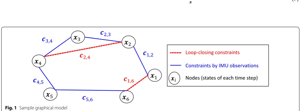
We treat the problem as an optimization of a graphical model shown in Fig. 1. The state at each time is modeled as a graph node. The constraints representing a relation between two nodes are modeled as graph edges.
Objective function
We define a vector containing all time-series state param-eters as follows:
This vector is used as an objective variable in our optimi-zation problem.
Next, given a set of constraints, we aim to find the opti-mal vector x∗ . Constraint cij is a nine-dimensional
vec-tor representing the state of xj relative to xi , which is
obtained from IMU measurements and prior knowledge about the target motion. The problem is formulated as the maximization of the posterior density as follows:
Assuming that the errors in the constraints are statisti-cally independent of each other and Gaussian, we can express the posterior density as follows:
where f(x|µ,�) is the probability density function of the
normal distribution N(µ,�) and eij(x) denotes the error
of the constraint cij.
By taking the logarithm of Eq. (6), the optimization problem can be rewritten as follows:
x:= [x⊤1,. . .,x⊤n]⊤.
(5) x∗=arg max
x
p(x|{cij}�i,j�∈C).
(6) p(x|{cij}�i,j�∈C)=
�i,j�∈C
f(eij(x)|0,ij),
(7) x∗=arg min
x
F(x),
Constraints
Each component (attitude, velocity, and position) in the constraint cij is denoted as u(ij),v(ij) , and t(ij) , respectively.
Two types of constraints are employed: a constraint between consecutive nodes ( j=i+1 ) and that between non-sequential nodes (loop-closing constraints). The former type of constraints can be calculated using IMU measurements as follows:
In contrast, the non-sequential constraints can be obtained from prior knowledge about the motion or observations with external sensors. The single constraint used in Sagawa et al.’s method is given in this form. For example, a constraint that the initial (time t=0 ) and final (time t=n ) states are identical can be expressed as
follows:
Error function
We define the error function as follows:
The error function returns a zero vector when the state of node j relative to node i matches cij.
Optimization
We employ the Gauss–Newton method to minimize function F in Eq. (8). This method is a gradient descent method that can be used for nonlinear least-squares problems. We initiate the objective variable with an ini-tial estimate, xˆ , and iterate over the following three steps
until convergence:
1. Linearization: Calculate F¯xˆ(d) , i.e., the linear approx-imation of F(x) at x=xˆ.
2. Minimization: Determine the update vector d , which
minimizes F¯xˆ(d).
3. Update: Update the current estimate xˆ using d.
Linearization
In the first step, we obtain the linearized objective func-tion F¯xˆ(d) as follows:
(8)
F(x):= �i,j�∈C
eij(x)⊤ijeij(x),
(9) ij :=−ij1.
cij=
ωi�t
(Riai−g)�t
vi�t
.
c0,n= [0, 0, 0, 0, 0, 0]⊤.
eij(x):=
(−u(ij))∗(−ui)∗(uj) −v(ij)+vj−vi
−t(ij)+tj−ti
.
Here, Jij is the Jacobian matrix of eij(x) at x=xˆ.
The linearized objective function F¯xˆ(d) can be expanded into a quadratic function as follows:
Minimization
By setting the derivative of Eq. (10) to zero, the minimizer ˆ
d is obtained by solving the following linear equation:
H is a 9n × 9n matrix, and it grows rapidly as the
num-ber of nodes increases. Therefore, naive methods, includ-ing Gauss–Seidel minimization, require a large amount of time for computations. Since H is symmetric,
posi-tive-definite, and sparse (i.e., the number of loop-closing constraints is small), the linear system can be efficiently solved via sparse Cholesky decomposition or the precon-ditioned conjugate gradient method [10, 11].
Update
Finally, using the obtained minimizer dˆ , we update the
current estimates using the following equation:
Relevance to graph‑based simultaneous localization and mapping
The formulation can be considered as an extension of graph-based simultaneous localization and mapping (SLAM) [12, 13]. Graph-based SLAM produces atti-tude and position estimates, and the proposed method extends the state vector with velocity as an extra degree of freedom.
Improving initial estimates
The computational cost of the proposed method is higher than those of the graph-based SLAM methods for the same number of nodes and constraints as H becomes
larger. Therefore, to achieve practical processing time,
F(xˆ+d)= �i,j�∈C
eij(xˆ+d)⊤ijeij(xˆ+d)
≈
�i,j�∈C
(eij(x)ˆ +Jijd)⊤ij(eij(x)ˆ +Jijd)
:= ¯Fxˆ(d).
(10) ¯
Fxˆ(d)=d⊤H d+2b⊤d+const.,
(11)
where
H :=
�i,j�∈C
J⊤ijijJij,
b:=
�i,j�∈C
eij(x)ˆ ⊤ijJij.
(12)
H d = −b.
(13) ˆ
we employ an initialization technique, which is described below.
The positions estimated via simple integration are typi-cally far from the optimum value. If we begin optimiza-tion with such poor initial estimates, the optimizaoptimiza-tion will require a large amount of time to converge.
Therefore, we improve the initial estimates by solv-ing a sub-problem. The sub-problem employs the same graph-based formulation as the main problem and only optimize the attitude and velocity estimates. More specifically,
is used as an objective variable. The attitude and velocity components of the constraints were also extracted and employed.
We initialize the position estimates for the main prob-lem by integrating the attitudes and velocities returned by sub-problem optimization, thereby reducing the itera-tions required for convergence in the main optimization problem.
Results
Simulation experiments
Experiments with simulated data were conducted as follows. IMUSim [14] was employed to generate 100 different random trajectories with ideal 100-Hz IMU measurements. The duration of each generated trajectory was 3 s.
To improve the realism of the simulation, artificial white noise was added to the ideal measurements. The standard deviations of the noise terms were 0.1 m/s2 for
acceleration and 0.3°/s for angular velocity. Bias errors of 0.2°/s were also added to the angular velocity data.
First, we tested the processing methods for motions with only one constraint. The estimation accuracy of the
x′:=u⊤0,v⊤0,u1⊤,v⊤1,. . .,u⊤n,v⊤n ⊤
proposed method was compared with those of the naive integration and Sagawa et al.’s conventional method [8].
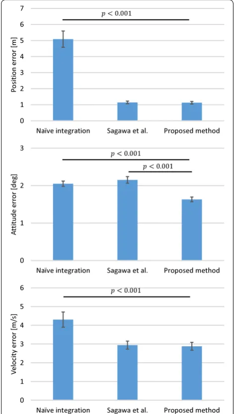
The examples of estimated trajectories and RMS errors of each method are shown in Fig. 2 and summarized in Fig. 3. Regarding position and velocity estimations, the proposed method returned errors that were almost same as those returned by the other methods, which makes sense because both methods used the same information.
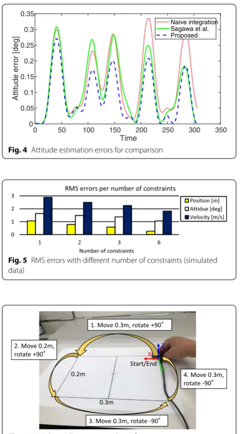
However, the proposed method exhibited significantly smaller attitude errors in comparison with Sagawa et al.’s method ( p<0.001 using the Wilcoxon signed-rank test). The typical attitude estimation results are plot-ted in Fig. 4, which is generated using the same motion as shown in Fig. 2. This plot shows that both correction
Fig. 2 Sample trajectory estimation result
methods accurately estimated the final attitude; however, Sagawa et al.’s method exhibited larger errors for inter-mediate states. This was because the method uniformly distributed the attitude errors along a single rotation axis. Thus, the correction was not expected to necessarily match with the direction of the errors.
Next, we tested the method with multiple constraints. Several observation points were chosen in the simulated data sequences, and the true IMU states at these points were used as additional constraints. The relation between the number of constraints used and the estimation accu-racy is summarized in Fig. 5. This figure clearly shows that the estimation accuracy improves as the number of constraints increases.
Trajectory estimation using real IMU data
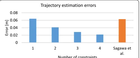
The accuracy of trajectory estimation was evaluated using real IMU data collected with an Xsense MTi-3 IMU at 100 Hz. The motion measured is shown in Fig. 6. The IMU was moved to four vertices of a 0.3 m × 0.2 m
rectangle and returned to the initial position and orien-tation. The motion lasted approximately 7 s. To perform the calibration of the IMU’s acceleration and angular velocity bias, approximately 3.0 s of motionless time was included at the beginning of the motion.
We again compared the proposed method and Sagawa et al.’s method [8] in terms of estimation accuracy. Both methods were provided the same constraint, i.e., the ini-tial and final states were identical. Extra constraints were employed in the proposed method, which are defined by the relative positions of three vertices and the assump-tion that the device stops moving at these vertices. The times when the IMU visited the vertices was calculated based on the acceleration spikes caused by collisions with the table surface.
The estimated 3D trajectories were projected into a two dimensional plane (Fig. 7) for comparison with the reference trajectory. The Fréchet distance (a similarity measure) between the estimated trajectory and reference trajectory was employed for measuring errors. The errors were 0.062 m from Sagawa et al.’s method and 0.022 m from the proposed method.
The changes in the estimation accuracy for different number of constraints are plotted in Fig. 8. This figure shows that the estimation accuracy improves as the num-ber of constraints increases.
The processing times for the proposed method and Sagawa et al.’s method were 0.58 and 0.022 s, respectively, on a laptop equipped with a Core i7-7600U processor
0 50 100 150 200 250 300 350 Time
0 0.05 0.1 0.15 0.2 0.25 0.3 0.35
Attitude error [deg
]
Naive integration Sagawa et al. Proposed
Fig. 4 Attitude estimation errors for comparison
Fig. 5 RMS errors with different number of constraints (simulated data)
Fig. 6 IMU data collection procedure of trajectory estimation experi-ment
(mean of 10 trials). Although the proposed method per-formed slower than Sagawa et al.’s method, the perfor-mance of our method does not appear to be a significant problem for the purpose of offline motion analysis.
Attitude estimation using real IMU data
The attitude estimation accuracy was also evaluated using the MTi-3 IMU. In this evaluation, the IMU was rotated randomly and returned to the initial state, as depicted in Fig. 9. The constraint that the initial and final states are identical was employed. The mean attitude errors for the collected 53 sequences of the IMU data are shown in Fig. 10. As can be seen from the figure, the estimation error of the proposed method was smaller than that of Sagawa et al.’s method ( p=0.0376).
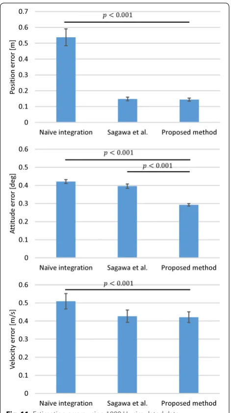
Analysis of the effect of data frequency and length
To evaluate how the data acquisition rate affects the performance of the proposed method, we conducted an additional experiment using simulated IMU data of 1000 Hz from the same 100 random motions employed in the abovementioned simulation experiments. The estimation results are summarized in Fig. 11. The graph shows similar trend with that of 100 Hz (Fig. 3). The mean processing time of the proposed method was 3.4 s
for 1000 Hz data and it is 15 times slower than that for 100 Hz (0.23 s).
The estimation accuracy for longer motions was evalu-ated using the same settings as the trajectory estimation experiments using the MTi-3 IMU. Two additional data sequences were collected by slowly moving along the rectangle (same procedure as shown in Fig. 6); the dura-tion of the data was approximately 14 and 21 s. Trajec-tory estimation results are summarized in Fig. 12. It was observed that the estimation accuracy of both the pro-posed method and Sagawa et al.’s method degraded rap-idly as motion length increased.
Conclusions and future work
Using IMU data, the proposed motion estimation method corrects the accumulated errors via least-squares fitting with constraints that are obtained from IMU measurements and from prior knowledge of the motion. This method can incorporate more than one constraint in error correction steps, thereby improving the estima-tion accuracy. The effect of accuracy improvement was
Fig. 8 Trajectory estimation errors with different number of con-straints (real IMU data)
Fig. 9 IMU data collection procedure of attitude estimation experiment
0.4403 0.4748
verified by experiments using simulated and real data. When using a single constraint, the proposed method estimated attitude more accurately than the conventional methods. The computation time of the proposed method was practical for motions with duration of several
seconds, thanks to the use of an initialization technique. Nevertheless, the computational cost will be large on data with long duration or high frequency. One way to alleviate the problem would be node thinning.
In future work, we plan to apply this method to actual sports data. An analysis of table tennis rallies is in progress.
The proposed method has a limitation: it assumes that the constraints are independent; however, biased meas-urements can violate this assumption. A mathematical model that considers gyroscope and accelerometer biases can compensate for this limitation.
Authors’ contributions
The author read and approved the final manuscript.
Competing interests
The author declares that he has no competing interests.
Ethics approval and consent to participate Not applicable.
Appendix
Rotation vector definition
A rotation vector is a 3D vector representing a 3D rota-tion. It can be calculated from a 3D unit vector represent-ing the rotation axis a= [ax,ay,az]⊤ and the angle of
rotation θ[rad] as follows:
The inverse rotation can be calculated as follows:
For brevity, the norm of v is denoted as v.
Conversion between unit quaternion
Conversion from a rotation vector to unit quaternion q= [qw,qx,qy,qz]⊤ can be expressed as follows:
Conversion from unit quaternion to rotation vector can be expressed as follows:
Rotation vector to rotation matrix
A rotation vector can be converted to a rotation matrix as follows (Rodrigues’s formula):
(14)
v:=θa.
(15) v−1= −v.
(16) qv(v):=
cosv2
v1
v sinv2
v2
v sin v
2
v3
v sinv2
.
(17) vq(q):=
2 arccos(qw)
� 1−q2
w
qx
qy
qz
.
(18)
R=I3+sinvK+(1−cosv)K2,
Fig. 11 Estimation errors using 1000 Hz simulated data
Rotation vector multiplication
The product of the two rotation vectors v and u is repre-sented by v∗u , which is calculated in terms of the
qua-ternion product.
This operation represents the concatenation of two rota-tions (first rotation by v , and the next rotation by u).
Derivatives of rotation vector multiplication
Derivatives of three rotation vector multiplication are calculated as follows:
Here, H, G, Q, and Q¯ are given as follows [9]:
wherec:= 11 −q2
w, d:=
arccos(√ qw) 1−q2
w
,
whereS:=sinv2, a:=vcosv2−2S,
(19)
K :=1 v
0 −v3 v2
v3 0 −v1
−v2 v1 0
.
(20)
v∗u:=vq(qv(v)qv(u))
(21)
∂(u∗v∗w)
∂v =H(qv(u∗v∗w))Q(q
u)¯
Q(qw)G(v)
:=U2(u,v,w),
(22)
∂(u∗v∗w)
∂w =H(qv(u∗v∗w))Q(q
u)
Q(qv)G(w)
:=U3(u,v,w).
(23)
H(q):= ∂vq(q) ∂q
=
2cqx(dqw−1) 2d 0 0
2cqy(dqw−1) 0 2d 0
2cqz(dqw−1) 0 0 2d
,
(24) G(v):=∂qv(v)
∂v = S 2v
−v1 −v2 −v3
2 0 0
0 2 0
0 0 2
+ a 2v3
0 0 0
v12 v1v2 v1v3
v1v2 v22 v2v3
v1v3 v2v3 v32 , (25)
Q(q):=
qw −qx −qy −qz
qx qw −qz qy
qy qz qw −qx
qz −qy qx qw
,
Jacobian matrix calculation
The Jacobian matrix of eij(x) at x= ˆx has the following
sparse structure:
Here, J(i)ij and J(j)ij are the partial derivatives of eij(x) by xi
and xj , respectively, and they can be calculated as:
Publisher’s Note
Springer Nature remains neutral with regard to jurisdictional claims in pub-lished maps and institutional affiliations.
Received: 31 January 2018 Accepted: 16 May 2018
References
1. Seaman A, McPhee J (2012) Comparison of optical and inertial tracking of full golf swings. Procedia Eng 34:461–466
2. TruSwing™. http://www.garmi n.com.hk/produ cts/intos ports /trusw ing/ (26) ¯
Q(q):=
qw −qx −qy −qz
qx qw qz −qy
qy −qz qw qx
qz qy −qx qw
.
Jij=
· · ·0· · ·J(i)
ij · · ·0· · ·J (j) ij · · ·0· · ·
.
(27) J(ijj):=∂eij(x)
∂xj � � �
x=ˆx
= ∂ ∂xj
(−u(ij))∗(−u
i)∗(uj) −v(ij)+v
j−vi
−t(ij)+t
j−ti � � � �
x=ˆx
=
∂ ∂xj(−u
(ij))∗(−u
i)∗(uj) � �
x=ˆx 0 0
0 I3 0
0 0 I3
=
U3(−u(ij),− ˆui,uˆj) 0 0
0 I3 0
0 0 I3
,
(28) J(i)ij :=∂eij(x)
∂xi
� � �
x=ˆx
= ∂∂
xi
(−u(ij))∗(−ui)∗(uj)
−v(ij)+vj−vi
−t(ij)+tj−ti
� � � �
x=ˆx
=
∂
∂xi(−u(ij))∗(−ui)∗(uj)
� �
x=ˆx 0 0
0 −I3 0
0 0 −I3
= −
U2(−u(ij),− ˆui,uˆj) 0 0
0 I3 0
0 0 I3
3. Smart Tennis Sensor for Tennis Rackets. https ://www.sony.com/elect ronic s/smart -devic es/sse-tn1w
4. Woodman OJ (2007) An introduction to inertial navigation. Technical report, University of Cambridge
5. Madgwick SOH, Harrison AJL, Vaidyanathan R (2011) Estimation of IMU and MARG orientation using a gradient descent algorithm. In: IEEE inter-national conference on rehabilitation robotics, pp 1–7
6. Ojeda L, Borenstein J (2007) Non-GPS navigation for security personnel and first responders. J Navig 60(3):391–407
7. Sagawa K, Ohkubo K (2015) 2D trajectory estimation during free walking using a tiptoe-mounted inertial sensor. J Biomech 48(10):2054–2059 8. Sagawa K, Abo S, Tsukamoto T, Kondo I (2009) Forearm trajectory
meas-urement during pitching motion using an elbow-mounted sensor. J Adv Mech Design Syst Manuf 3(4):299–311
9. Diebel J (2006) Representing attitude: Euler angles, unit quaternions, and rotation vectors. Report, Stanford University
10. Konolige K, Grisetti G, Kummerle R, Burgard W, Limketkai B, Vincent R (2010) Efficient sparse pose adjustment for 2D mapping. In: Proceed-ings of the IEEE international conference on intelligent robots & systems (IROS), pp 22–9
11. Montemerlo M, Thrun S (2006) Large-scale robotic 3-D mapping of urban structures. In: Ang MH, Khatib O (eds) Experimental robotics IX: the 9th international symposium on experimental robotics, vol 21. Springer, Berlin, pp 141–150
12. Lu F, Milios E (1997) Globally consistent range scan alignment for environ-ment mapping. Auton Robots 4:333–349
13. Grisetti G, Kummerle R, Stachniss C, Burgard W (2010) A tutorial on graph-based slam. IEEE Intell Transp Syst Mag 2(4):31–43