Digital spotlighting filtering optimization for SAR imaging

R E S E A R C H

Open Access

Digital spotlighting filtering

optimization for SAR imaging

Eric J. Balster

, David B. Mundy

, Andrew M. Kordik

and Kerry L. Hill

Abstract

In this paper, a synthetic aperture radar (SAR) image formation simulator is used to objectively evaluate the parameter selection within the digital spotlighting process. Specifically, recommendations for the filter type and filter order of the low-pass filters used in the range and azimuth decimation processes within the digital spotlighting algorithm are determined to maximize image quality and minimize computational cost. Results show that a finite impulse response low-pass filter with a Taylor(n=5)window applied provides the highest image quality over a wide range of filter orders and decimation factors. Additionally, a linear relationship between filter length and decimation factor is found.

Keywords: Spotlight SAR simulator, Digital spotlighting, Filter order, Filter windowing

1 Introduction

Of the several methods for synthetic aperture radar (SAR) image formation, back-projection has many attrac-tive attributes. A SAR image may be iteraattrac-tively formed by back-projecting each pulse return independently and using a simple summation of the back-projected returns to form the SAR image. Thus, each pulse return may be processed in parallel. Additionally, the back-projection process automatically ortho-rectifies the image allowing for ease of geo-location of the processed imagery. How-ever, there is a significant computational cost to back-projection. Although it is a conceptually straightforward algorithm, it carries a computational complexity ofO(N3) which does not scale.

A common way to combat the non-scalable nature of the back-projection algorithm is to break the SAR phase history into manageable pieces and back-project differ-ent locations of the SAR image independdiffer-ently. This pro-cess, called digital spotlighting [1], lends itself to further parallel processing and scalability of the back-projection algorithm.

Several methods in the literature have used digital spot-lighting in SAR image formation. In [2], a new algorithm

*Correspondence:[email protected]

1_{Department of Electrical and Computer Engineering, Kettering Laboratory,} University of Dayton, Rm. 341, 300 College Park, Dayton, OH 45469, USA Full list of author information is available at the end of the article

for circular SAR imaging is developed using digital spot-lighting for acceleration. Additionally, in [3], digital spot-lighting is used to enhance the back-projection process in terms of reduced Doppler aliasing. In [4], digital spot-lighting is used to processes wide bandwidth and wide beamwidth P-3 SAR data.

However, many of the methods provided in the litera-ture do not give guidance on several of the parameters involved in the digital spotlighting process, namely filter order and filter type. The choice of filter and the length of its impulse response play a large role in the formed SAR image quality and the computational complexity of the digital spotlighting algorithm.

This paper presents a series of tests to determine fil-ter design guidelines for digital spotlighting in the SAR image formation process. A SAR image formation simu-lator is used which generates synthetic SAR video phase history (VPH) from digital imagery [5,6]. The synthetic VPH data is then formed into SAR imagery via digital spotlighting, inverse Fourier transform (iFFT) processing, and back-projection. Because the synthetic VPH is gen-erated from digital imagery, the quality of the formed SAR imagery is able to be objectively evaluated with well-known image processing metrics. In this study, structured similarity (SSIM) is used to provide simple guidelines on filter design in SAR digital spotlighting [7].

Test results show that a finite impulse response (FIR) filter Taylor window(n = 5)provides the highest image

Fig. 1SAR simulator processing overview

quality over several windowing methods tested, and a sim-ple linear relationship between the number of digitally spotlit segmentsDand filter orderMis discovered.

Following the introduction, Section 2 provides an overview of the SAR simulator for image formation. Section3provides a detailed overview of the digital spot-lighting algorithm. Section4shows the results of FIR filter window evaluation, and Section5provides an evaluation of the filter order. Section 6 provides some concluding remarks.

2 SAR processing overview

In order to objectively evaluate different parameters of the digital spotlighting processing chain, a spotlight SAR simulator is used to generate synthetic VPH from digital imagery. Then, traditional SAR processing methods are used to generate imagery from the synthetic VPH data. Because the synthetic VPH is generated from imagery,

traditional image processing metrics may be used to objectively evaluate the processing methods. Figure 1

gives a block diagram of the SAR simulator process. As shown in Fig.1, the SAR simulator is comprised of six processing steps. The first set of processing steps in the simulator form the VPH from a digital image I[·]. This set of functions are referred to as theradar process-ing functions. TheCalculate Rangefunction determines the range from the beginning of the imaging patch to each pixel in the image,d[h,v,θ], whereθ is the angular posi-tion of the radar with respect to the image. TheGenerate Return function sums up delayed and scaled linear fre-quency modulated (LFM) pulses to form the return SAR signal, given by:

xret(t,θ)=

i,j

Is[i,j]xp

t−2d[i,j,θ] c

, (1)

where xp(t) is the emitted radar pulse, and Is[·] is the

digital imageI[·] scaled in magnitude.

TheDemodulate, Sample, and Matched filterfunction is a set of standard SAR processing techniques to generate the VPH fromxret(t,θ). The synthetic VPH is labeled as

Xph[k,θ] in Fig.1.

The next set of functions are referred to asimage pro-cessingfunctions. These functions take the synthetic VPH data and form SAR imagery. The first image processing function is the digital spotlighting function. This func-tion allows segmentafunc-tion of the VPH data so that different sections of the imaging scene may be formed indepen-dently. The next process is the iFFT and Oversample function which utilizes the inverse fast Fourier Transform to convert the VPH data into a range profile, Rp[k,θ].

The final image processing function is theback-projection function which paints the range profile over the imaging scene, provides phase error correction, and sums up each back-projected pulse return to form the SAR image.

Each of the processing functions given in Fig. 1 is developed in detail in [8], with the exception of digital spotlighting, which is detailed in Section3.

2.1 SAR dynamic range

Generally, SAR imagery is displayed in decibels due to its large dynamic range. Typical imagery, however, has a rel-atively limited dynamic range. Thus, to effectively utilize imagery in creating synthetic phase history, the dynamic range of the imagery is stretched. First, we can deter-mine the dynamic range of the radar by determining the number of bits in the A/D process.

RdB=20 log10(2−b), (2)

whereRdBis the resolution of the A/D converter in

deci-bels, and b is the number of bits resolved in the A/D converter. Consider we have an imageI[·], whereI[h,v], wherehis the horizontal pixel index (column), andvis the vertical index (row). To stretch the dynamic range of imagery, we have:

Is[h,v]=10(max(I[·])−I[h,v])

RdB

20 _{, (3)}

whereIs[·] is the stretched image. If the original image,

I[·], has a range of [ 0, 1], the scaled imagery Is[·] also

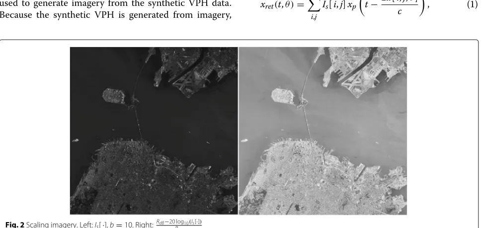
ranges from [ 0, 1]. However, its dynamic range is shifted to match that of the A/D converter. Figure 2 gives an

example of the “San Francisco” image scaled tob = 10 (i.e.,RdB= −60.21).

As shown in Fig. 2, the scaled imagery is then best visualized in decibels.

3 Digital spotlighting method

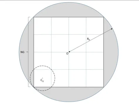
Assume a scene with alias-free imaging region of radius R0. From that scene, a SAR image of(NG)×(NG)meters

may be formed, where N is the number of row/column pixels, andGis the ground sample distance.

NG=√2R0. (4)

BothNandGare determined by:

G= c

2BWp

, (5)

and

N= c

2√2Gf, (6)

whereBWp is the LFM pulse bandwidth,f = T1r is the

frequency step size, Tr is the duration of the return

sig-nal, andcis the speed of light. A depiction of the imaging region is given in Fig.3.

One of the uses of digital spotlighting is to mitigate the computational burden of back-projection of the SAR VPH to image the scene. Since back-projection is an O(N3) algorithm, it does not scale, so digital spotlighting is a way to break up the phase history into computationally manageable sections for imaging via back-projection.

Given the imaging scene in Fig. 3, the original imag-ing canvas is N×N pixels. Through digital spotlighting, D2digitally spotlit segments are back-projected to form

N

D×NDpixel images. First, the central position of each

of the the digitally spotlit scenes, given by Ci,j, is

deter-mined. The digitally spotlit scenes are indexed byiandj row and column indices (i.e.,i,j∈[ 0,D−1]). The center

Fig. 5Filter windowing results

Fig. 7Zoomed in portion of Fig.6

of the digitally spotlit scene(i,j)is given by:

hC(i,j)= 2j+₂1N_D

vC(i,j)= 2i+₂1N_D

. (7)

The pixel locations are converted to distances to the cen-ter of the imaging scene (scene cencen-ter), indicated byOin Fig.3, by:

dh(i,j)=

hC(i,j)− N₂

G dv(i,j)=

_N

2 −vC(i,j)

G. (8)

Digital spotlighting consists of four major processing steps:

• Repositioning of the antenna

• Re-centering of the phase history data

• Decimation in the range dimension

• Decimation in the azimuth dimension

3.1 Repositioning of the antenna

For each pulse return of the phase history, the position of the antenna must be updated to reflect the position of the new scene center. Assume we have an antenna position of P = (X,Y,Z), whereX,Y, andZ are the latitude, longi-tude, and altilongi-tude, respectively, of the antenna, in meters. The new antenna position is, then, given by:

PC(i,j)=

Rx(i,j),Ry(i,j),Rz

, (9)

where

Rx(i,j)=X−XO+dh(i,j),

Ry(i,j)=Y−YO+dv(i,j),

Rz=Z−ZO,

(10)

andPO = (XO,YO,ZO)is the position of scene centerO.

When back-projecting the digitally spotlit area,PCis used

for all distance calculations.

Fig. 9Zoomed in portion of Figure8

3.2 Re-centering of the phase history data

Re-centering of the phase history data applies a phase shift in order to place the digitally spotlit scene at zero fre-quency. Because the phase history is frequency dependent upon range, the differential range from the center of the spotlit scene to scene center is first calculated.

R=(X−XO)2+(Y−YO)2+(Z−ZO)2

RC(i,j)=

Rx(i,j)2+Ry(i,j)2+R2z

dR(i,j)=RC(i,j)−R

. (11)

The re-centered phase history is then given by:

XC,i,j[k,θ]=Xph[k,θ]e−

j4πf[k]dR(i,j)

c _{, (12)}

where

f[k]=fc−

BWp

2 +fk. (13)

Xph[·] is the original phase history data of the scene, and

XC,i,j[·] is the re-centered phase history about position

Ci,j.f[k] are the frequency bins in range, wherek∈[ 0,K),

andKis the number of range samples inXph[·].fcis the

center frequency of the radar’s LFM pulse.

3.3 Decimation in the range dimension

The re-centered data is then low-pass filtered with a dis-crete cutoff frequency of π_D radians per sample, in which we obtain:

Xrlf,i,j[k,θ]=Fr XC,i,j[k,θ]

, (14)

whereFr{·}is the low-pass filtering operation in the range

dimension. Then, the low-pass-filtered data may be down-sampled by a factor ofD.

Xrd,i,j[k,θ]=Xrlf,i,j[Dk,θ] . (15)

X_rd,i,j[·] is the phase history decimated in range for spotlit area(i,j).

3.4 Decimation in the azimuth dimension

The alias-free azimuth resolution is used to determine the amount of decimation in the cross-range. The new azimuth step size is given by:

θn=

cD 4 cos(φ)R0

fc+BW₂p

, (16)

whereφ is the minimum elevation angle of the radar to the spotlit scene, given by:

φ =arctan Rz

maxRx(i,j)2+Ry(i,j)2

. (17)

The decimation factor in azimuth is given by:

L= _θ

n

θ

−1, (18)

and the decimated phase history used in back-projection of the digitally spotlit area is given by:

Xalf,i,j[k,θ]=Fa Xrd,i,j[k,θ]

, (19)

Xsp,i,j[k,θ]=Xalf,i,j[k,Lθ] . (20)

Fa{·} is the low-pass filtering operation applied in the

azimuth dimension, and Xsp,i,j[·] is the digitally spotlit

VPH for region(i,j). The digitally spotlit phase history can then be back-projected to form a subsegment of the origi-nal imaging scene, whose center isPC(i,j). The complexity

of the back-projection process of Xsp,i,j[·] is significant

reduction from the back-projection ofXph[·] considering

there are a factor of DLfewer samples in Xsp,i,j[·], and

those samples are projected onto an imaging plane which has a factor ofD2fewer samples.

4 Filter window results and discussion

A number of windowing functions have been used in the literature for SAR processing. In [9], a Hamming window is used on the LPF for digital spotlighting. Additionally, subsequent articles have used Taylor windows and raised cosine windows in different SAR processing techniques [10,11]. In the following study, six different windows are compared: rectangular, Hamming, Blackman, Taylor(n= 5), raised cosine, and Kaiser(β = 5). The Blackman and Kaiser windows are included due to their powerful stop-band suppression capabilities, and Taylor order(n = 5) and Kaiser (β = 5) parameters are set because those particular variants performed the best over a number of values tested.

In the study, four images are considered: “Stockton,” “San Francisco,” “Pentagon,” and “Washington, D.C.” All of the images can be found at [12]. Each image is a 1024×1024 color image, and they are converted to grayscale. Additionally, each image is cropped from the center to form four 512×512 grayscale images. Each of these eight images is fed into the SAR simulator with digital spotlighting enabled to test different variables of the digital spotlight processing. The converted grayscale images are given in Fig.4.

The simulator options are as follows: We definePO =

(0, 0, 0)andP= (3696, 1531, 2800)m at the center of the synthetic aperture.R0 = 707.1 m. All radar parameters,

number of pulses, and azimuth step size are determined by [13].

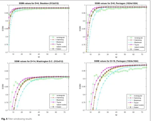
For image quality analysis, the Structured Similarity (SSIM) metric is used [7]. For filter window analysis, each of the windows is used over a range of filter orders on each of the test images. SSIM results are collected and analyzed over a range of D ∈[ 3, 20]. The filter length is 2M+ 1 where M ∈[ 5, 75] is incremented in steps of 2. Results for four of the images and different decimation factors are given in Fig.5.

In Fig. 5, two conclusions can be made. First, all win-dowing methods eventually result in good overall digital spotlighting performance with the exception of the rect-angular window. Regardless of filter order, the rectrect-angular window performs below that of the other windowing methods. Second, the Taylor window (n = 5) performs the best of the windows tested. Although only D ∈

{6, 8, 14, 18}digital spotlighting segments are shown for a few images in Fig.5, the Taylor window outperforms the others through the entire range of D =[ 3, 20] across all test images. We can visually see the effects of varying the type of filter window in digital spotlighting. Figure6gives a digitally spotlit “San Francisco” image with both rectan-gular and Taylor(n = 5)windowing applied. A zoomed in section of Fig. 6 is provided in Fig. 7. In addition to synthetic VPH, the AFRL GOTCHA phase history from a 2006 data collect [14] is processed with the simulator to validate the digital spotlighting process. The results of dig-ital spotlighting the GOTCHA dataset are given in Fig.8, with a zoomed in section given in Fig.9.

As shown in Figs.6 and7, when utilizing the rectan-gular window, aliased regions are prominent, and there are visual bordering effects at the intersection between spotlit regions. Conversely, when applying a Taylor(n = 5) window, these artifacts are significantly reduced and not readily visible. Additionally, we can see the improved image quality utilizing a Taylor window over a rectangular window in the GOTCHA data, provided in Figs.8and9.

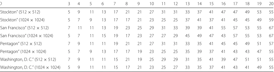
Table 1Masmfor various decimation factors and imagery

D 3 4 5 6 7 8 9 10 11 12 13 14 15 16 17 18 19 20

“Stockton” (512_×512) 5 9 11 13 17 21 21 27 31 31 33 37 41 47 47 49 53 55

“Stockton” (1024×1024) 5 7 9 13 17 17 21 23 25 25 37 41 37 41 45 45 49 59

“San Francisco” (512×512) 7 11 11 13 19 23 25 29 31 33 39 39 41 55 57 53 55 67

“San Francisco” (1024×1024) 5 7 11 15 19 17 23 27 27 29 45 49 47 43 57 55 53 67

“Pentagon” (512×512) 7 9 11 11 19 21 21 27 31 31 33 35 41 45 45 49 51 57

“Pentagon” (1024×1024) 5 7 9 13 17 17 19 23 25 25 35 39 37 41 43 43 47 55

“Washington, D. C.” (512×512) 7 9 11 11 15 21 19 25 29 29 31 35 41 39 47 51 51 55

5 Filter order results and discussion

An additional parameter for digital spotlighting is the fil-ter order, or length of the FIR filfil-ter’s impulse response in the decimation in range and azimuth. According to Kaiser’s FIR-length approximation, the required filter orderMis linearly proportional to the digital spotlighting segmentsD. Figure10shows SSIM values of the “Wash-ington D.C.” image across several filter orders and several decimation factors and applying a Taylor(n=5)window to the filter coefficients.

In Fig.10, it is readily shown that as the decimation fac-tor increases, the required filter orderMincreases as well. Careful analysis of these curves allow us to determine the minimum value of Mfor each decimation factor which maximizes the SSIM value. This filter order is referred to asMasm.Masmis defined as the minimum value ofM

where the SSIM score is greater than or equal to 0.99 of the maximum SSIM score over the range ofM(i.e., asymp-totically close to the maximum SSIM score). Table1gives Masmgenerated from all test images.

From the Kaiser FIR approximation, it is known that Masm linearly increases with increasingD. A linear fit is

applied to the data in Table1to create a simple calculation for the required filter order for digital spotlighting. Fitting the data to a line, we obtain:

Masm[D]= (sD+b)+0.5, D>1, (21)

where s = 2.95, and b = −4.15. Figure 11 gives a visual representation of the data in Table1and calculated

Masm[·].

As shown in Fig.11, the values forMasm over a fairly

wide range can be fairly well approximated with a lin-ear fit for each of the images tested. Thus, the FIR filter order required for digital spotlighting in general may be estimated using Eq.21.

Fig. 11Decimation factorD, verses filter lengthM, andMasm[·]

6 Conclusion

This paper presents an objective evaluation of fil-ter paramefil-ter selection for digital spotlighting in SAR imagery. The analysis is generated from a SAR image for-mation simulator which uses imagery to form the phase history of the radar. Because of this, the quality of the reconstructed SAR image may be objectively evaluated using well-known image processing metrics. From the analysis, it is shown that the Taylor window(n=5) pro-vides the best image quality over a wide range of filter lengths and decimation factors. Additionally a simple lin-ear relationship between the decimation factor and filter order is found.

Abbreviations

FIR: Finite impulse response; iFFT: Inverse Fourier transform; LFM: Linear frequency modulated; SAR: Synthetic aperture radar; VPH: Video phase history

Acknowledgements

The authors would like to thank the US Air Force Research Laboratory for funding this effort.

Authors’ contributions

The authors’ contributions to digital spotlighting processing are as follows: We have created a SAR simulator which can objectively evaluate different parameter selection of the digital spotlighting process, namely filter order and filter type used in the decimation of the VPH. We have additionally found a simple linear relationship between appropriate filter order and decimation factor. SAR processing developers can use this relationship to easily calculate the proper filter order to use for digital spotlighting. All authors read and approved the final manuscript.

Funding

Funding of this work was provided by the US Air Force Research Laboratory, Sensors Directorate.

Availability of data and materials

Images used in this study can be found at [12]. Additionally, the GOTCHA VPH data is available at [14].

Competing interests

The authors declare that they have no competing interests.

Author details

1_{Department of Electrical and Computer Engineering, Kettering Laboratory,} University of Dayton, Rm. 341, 300 College Park, Dayton, OH 45469, USA. 2_{University of Dayton Research Institute, 300 College Park, Dayton, OH 45469,} USA.3_{Sensors Directorate, United States Air Force Research Laboratory,} Wright-Patterson AFB, Dayton, OH 5433, USA.

Received: 28 March 2018 Accepted: 9 September 2019

References

1. M. Soumekh, inProceedings of 1st International Conference on Image Processing, vol. 1. Digital spotlighting and coherent subaperture image formation for stripmap synthetic aperture radar (IEEE, 1994), pp. 476–480 2. A. Dallinger, S. Schelkshorn, J. Detlefsen, Efficientω-k-algorithm for

circular SAR and cylindrical reconstruction areas. Adv. Radio Sci. 4.B.3, 85–91 (2006)

3. L. Nguyen, et al.,Enhancement of backprojection SAR imagery using digital spotlighting preprocessing(IEEE, 2004)

4. M. Soumekh, et al., Signal processing of wide bandwidth and wide beamwidth P-3 SAR data. IEEE Trans. Aerospace Electr. Syst.37(4), 1122–1141 (2001)

6. E. J. Balster, et al., inProceedings of the 5th International Workshop on OpenCL. Gpgpu acceleration using opencl for a spotlight sar simulator. (ACM, 2017), p. 1

7. Z. Wang, et al., Image quality assessment: from error visibility to structural similarity. IEEE Trans. Image Process.13(4), 600–612 (2004)

8. E. J. Balster, F. A. Scarpino, A. M. Kordik, K. L. Hill, Synthetic aperture radar imaging simulator for pulse envelope evaluation. J. Appl. Remote Sensing.11(4), 046022 (2017)

9. K. E. Dungan, L. A. Gorham, L. J. Moore, inAlgorithms for Synthetic Aperture Radar Imagery XX. Vol. 8746. SAR digital spotlight implementation in MATLAB (International Society for Optics and Photonics, 2013) 10. A. W. Doerry,Anatomy of a SAR impulse response. No. SAND2007-5042.

(Sandia National Laboratories, 2007)

11. C. V. J. Jakowatz, et al.,Spotlight-Mode Synthetic Aperture Radar: A Signal Processing Approach. (Springer Science & Business Media, 2012) 12. USC Signal and Image Processing Institute.http://sipi.usc.edu/database.

Accessed 31 July 2019

13. L. A. Gorham, L. J. Moore, inAlgorithms for Synthetic Aperture Radar Imagery XVII. Vol. 7699. SAR image formation toolbox for MATLAB (International Society for Optics and Photonics, 2010)

14. GOTCHA 2008 Dataset.https://www.sdms.afrl.af.mil/index.php? collection=gotcha. Accessed 31 July 2019

Publisher’s Note