O R I G I N A L P A P E R
Open Access
Planning urban pavement maintenance by
a new interactive multiobjective
optimization approach
Maria Grazia Augeri
1*, Salvatore Greco
2,3and Vittorio Nicolosi
1Abstract
Pavement maintenance is essential to prevent the deterioration of asset value and to satisfy the expectations of all stakeholders (objectives). However, the budgets are often insufficient to keep the road pavement at optimum levels. Therefore, a decision making process ought to be used for prioritizing different maintenance activities in order to achieve pre-defined goals by optimizing the use of the available budget. One of the biggest difficulties in multiobjective optimization method is the large number of the feasible solutions (Pareto optimal set or its approximation), which makes it hard for the Decision Maker to select the best solution.
To support interaction with the decision maker for identifying the best combination of maintenance actions,
this paper proposes a new methodology named “Interactive Multiobjective Optimization-Dominance Rough
Set Approach” (IMO-DRSA), using a decision-rule preference model.
The preference information, obtained by the Decision Maker (DM) during the course of the interaction, is processed using the Dominance-based Rough Set Approach in order to achieve a decision model expressed in terms of easily understandable “if ….then …” decision rules. This approach makes possible an interaction between the analyst and the decision maker and helps the decision maker to classify maintenance options and allocate limited funds according to predefined objectives (quantitative or qualitative). An application of the proposed methodology to road pavements of an Italian urban sub-network is presented.
Keywords: Pavement management, Multi-criteria decision-making, Maintenance, Rehabilitation, Road performance
1 Introduction
Efficient sustainable rural, urban and inter-urban port infrastructure in combination with affordable trans-port services drive commerce, mobility and access to social services and underpin development in all countries. Roads, averaging 80% worldwide, dominate the transport sector in many countries and are the principal means of passenger and freight movement. As matter of fact, in de-veloped countries, the road network constitutes one of the largest public assets. By way of example, the EU road net-work comprises about 5,5 million km of paved roads, and the total investment in transport infrastructure during the period 2000–2006 was€859 billion [1].
Despite the key role that road infrastructure plays in economic and social development, the tendency to give priority to new construction, the lack of understanding of the importance of maintenance, and chronic under-funding (imbalance between the rate of deterioration and the level of funding allocated) risk quickly jeopardis-ing this valuable asset, which has been built in developed countries over the past 70 years.
Road administrations have the difficult task of main-taining, operating, improving and preserving roads, at the same time, carefully managing the limited financial and human resources. Asset management has been widely accepted by central and local governments/ad-ministrations as a means to deliver a more efficient and effective long term approach to the management of highway infrastructure. This approach enables a better use of resources, while fulfilling legal obligations, deliv-ering stakeholder, social and environmental needs, and
* Correspondence:[email protected]
1Department of Enterprise Engineering, University of Rome“Tor Vergata”, Via
del Politecnico 1, 00133 Rome, Italy
Full list of author information is available at the end of the article
safeguarding the value of the network. To achieve stra-tegic asset management objectives, optimal maintenance and rehabilitation (M&R) programs must be defined and implemented over a planning horizon for system facil-ities (road pavements, footways, bridges, tunnels, etc).
In a traditional approach to asset management, opti-mal M&R programs are identified for each “sub-asset” (system facility) in the road transport system, more or less separately, but using the same strategic objectives and with the aid of a decision support system. Pavement is a significant component (sub-asset) of infrastructure systems, so that pavement maintenance and rehabilita-tion accounts for on average 40% (ranging from 19% to 65%) of total maintenance and operation expenses in Europe [2]. Software tools, referred to as pavement man-agement systems (PMS), have been used to support road administration in finding the best M&R plans (what treatment, when, and where) since the 1980s. All these systems have similar framework consisting of a central database, performance and cost models, and a decision support element (DSE). The DSE assists decision makers in determining pavement network work plans, which allow them to best meet the defined objectives under budgetary and other agency constraints, while taking into account the evolution of pavement performance.
Since the invention of the first PMSs, prioritization (ranking) or optimization models have been used in the DSE to face the problem of determining pavement M&R plans. In the approach based on prioritization, M&R re-sources are allocated by ranking all the pavement sec-tions on the basis of one or more parameters (e.g. road class, traffic volume, etc.), which are evaluated based on current year condition data. Therefore, this approach does not assure the selection of the best possible M&R strategy, nor does it allow multi-year programming.
The optimization approaches applied in the last cen-tury determined optimal maintenance pavement strat-egies using a single objective (e.g. minimizing costs or maximizing performance) and multiple constraints across one or more years of the analysis scope due to the fact that single objective optimization problems can be easily solved mathematically by linear or nonlinear programming. In order to integrate technical and eco-nomic aspects, cost-effectiveness (CE) and cost-benefit (CB) methods were extensively used in single objective optimization problems. Both CE and CB are analytical ways of comparing different forms of input or output, in this case by giving them money values, and could be regarded as an expedient multi-criteria analysis.
The main limitation of this approach is that it may be difficult to quantify in economic terms some social and environmental objectives identified in the asset manage-ment strategy [3,4]. A possible approach for the integra-tion of all strategic aspects is the use of multiobjective
optimization (MOO) methods. Due to the complexity of these methods, applications have got off the ground slowly, as data are often lacking and the methods are not easy to apply.
Many researchers [5, 6] have discussed the applica-tions and performance of optimization techniques when dealing with decision-making problems in road mainten-ance. Generally, in multiobjective optimization problems there is no one solution that is better than any other for all the considered objectives. In order to obtain a good solution to these problems, the concept of“Pareto opti-mality”was applied. A possible solution to a multiobjec-tive optimization problem is “Pareto optimal” if there is not another possible solution that improves one object-ive without worsening at least one other objectobject-ive [7]. Mathematically, all the Pareto optimal points are alike good solutions of the optimization problem. However a desirable outcome, for the decision maker, would be to select only one solution, from a set of Pareto optimal so-lutions, basing on his/her own judgment or preference. Depending on the role of the DM in preferences articu-lation, MOO methods can be categorized in methods with a priori articulation of preferences, methods with a posteriori articulation of preferences and interactive methods, as better explained in the following.
In this paper, the authors propose the application of new interactive MOO methods for road maintenance management. The MOO method combines the “ Inter-active Multiobjective Optimization” (IMO) with the
“Dominance-based Rough Set Approach” (DRSA) [8– 10] and is based on the idea of constrain the set of feasible solution, in the Pareto front, using some tar-get value of objective function (lower bound or upper bound in case of minimization) which result from the preference of DM.
2 Literature review
Multiobjective optimization has been widely used to allocate resources in pavement management and a large number of papers are present in literature about this topic. Some authors [3, 11] presented a good de-scription of multiobjective optimization technics ap-plied to this field.
The review presented below is not a comprehensive one, but only a description of the main approaches which have appeared in the literature, with the aim to describe their features, advantages and weakness, and to compare them with the proposed method.
as the one that corresponds to the ‘best’ value of the weighted sum. The main advantage of the WSM is the simplicity of its implementation and many researchers applied therefore this method [12, 13]. Its main weaknesses are the need for normalization, to solve multi-dimensional problems, and the subjectivity in-volved in setting weights and in the formal understand-ing of the decision maker’s preferences.
Other authors [14,15] have proposed to adopting mul-tiattribute utility theory, which is an axiomatized math-ematical framework for analyzing and quantifying choices involving multiple competing outcomes. The main advantages of this method are its ability to quantify the preferences of the DM and the easiness of combing it with other optimization methods. Instead, its weakness can be found in the difficulty it has in constructing the utility function in a practical situation, primarily because as it has numerous input needs and preferences have to be precise.
In other studies, analytic hierarchy process (AHP) was used. The method is based on obtaining preferences or weights of importance to the criteria and alternatives. The major characteristic of the AHP method is the use of pair-wise comparisons, which are used both to com-pare the alternatives with respect to the various criteria and to estimate criteria weight. In this method, both cri-teria and alternatives can be structured in a hierarchical way. This approach was applied in the field of pavement management by some authors [16–19]. The main advan-tage of this method is how easy it is to use, due to the use of pairwise comparisons that allow decision makers to weigh coefficients and compare alternatives with rela-tive ease. Moreover, it is scalable and can easily be ad-justed in size to accommodate decision making problems due to its hierarchical structure. The main limitation of AHP is the necessity of complex and time-consuming computation [20] in situation in which a large number of alternatives have to be considered. Additionally, it can lead to biased outcomes.
Artificial intelligence techniques, such as genetic-algorithm-based procedures, are also used for solving the multi-objective optimization problems. The main reason for the widespread of these methods is their cap-ability of providing good solutions both in the case of simple linear optimization problems or in that of diffi-cult combinatorial optimization problems. Several appli-cations appear in the literature [21–27]. The weaknesses of this method are its relatively high computational cost, the high programming complexity required and limited capacity to fine-tune solutions. To improve the perform-ance of the evolutionary algorithms in terms of effi-ciency, in some research studies a combination of genetic algorithm with local search heuristics, named
“memetic algorithms”was proposed [28].
No method can be considered better than another method. Rather, it is opportune to analyse the advan-tages and disadvanadvan-tages of each method in order to choose the one best suited to solve a specific problem.
Considering the specific issues related to pavement management process and some limitations observed in the most commonly used methods, in this paper the possibilities of applying a new method (IMO-DRSA), never applied in the field of pavements management, have been assessed [29].
A detailed description of the IMO-DRSA and its ad-vantages compared to other more commonly used methods is presented in the following sections.
3 Methods
3.1 Basic concepts about multiobjective methods for determining optimal pavement network work plans In multi-year multiobjective optimization, the goal is to identify a multi-annual works plan that can best meet the multiple objectives and the constraints (e.g. budget). In the multi-annual works plan a set of strategies are ap-plied to the road network (i.e. a set of individual road sections). Strategys(among a set of possible strategiesS, withs∈S) is usually defined as a series of required treat-ments initiated every yeartwithin the time period T of the analysis scope (with t∈T). To make the complexity of the problem manageable, the set of possible treat-ments for each road section can be restricted by utilizing decision trees (or other methods) in order to identify a reasonable subset of possible treatments. Therefore, the strategy may be considered the application of a mainten-ance decision criteria (e.g. decision tree) to define a series of treatments during the periodTon a section.
The problem may be expressed in mathematical terms as follows:
Minimize or maximize F(x) = [F1(x), F2(x), …, Fk(x)]T subject to gj(x)≤0, j = 1, 2,…, m, and hl(x) = 0, l = 1, 2,…, e,
where
k is the number of objective functions, m is the num-ber of inequality constraints, and e is the numnum-ber of equality constraints.
x∈En is a vector of design variables (also called deci-sion variables), and n is the number of independent vari-ables xi(is the strategy applied in the road section i).
conflicting goals. Essentially, a vectorx∗∈X is said to be Pareto optimal for a multi-objective problem if all other vectorsx∈X have a higher value for at least one of the objective functions Fi, withi= 1, …,k, or have the same value for all the objective functions. Therefore, you only dispose of a partial order among solutions and need extra preference information coming from the decision maker to be able to select the most preferred solution for the problem involving multiple conflicting objectives. Then the approaches existing in the literature to solve such problems can be categorized depending on how the decision-maker articulates these preferences and the fol-lowing classification into three families is usually adopted [30]: a priori preference methods, progressive preference methods, a posteriori preference methods.
In the “a priori preference methods” the decision maker defines the trade-off to be applied before run-ning the optimization methods (e.g. constraint method or aggregative methods where the objective functions are gathered into one objective function like a weighted sum).
The “a posteriori” approach is composed of two phases; in the first phase, a specialized algorithm is used to search for a representative set of trade-offs between a generally small number of objectives. In the second phase, the decision maker picks a final solution from that set using higher order preferences, which were not expressed explicitly in the objective functions.
In the “progressive preference methods” the decision maker improves the trade-off to be applied during the running of the optimization (e.g. interactive method be-long to this family). Unlike a posteriori techniques, which work in batch mode, an interactive method pre-sents information sparingly to the user and gets refined preferences from him/her in return.
Some multiobiective optimization methods exist, which do not fit exclusively into one family. For ex-ample, an “a posteriori” approach mixed with an inter-active method can be used.
The objective of this work is to present how the IMO-DRSA method can be efficiently used as decision support tool to develop pavement maintenance plans at network level in a multiobjective PMS, which is fully in-tegrated in an asset management system.
3.2 Interactive multiobjective mixed-integer optimization using dominance-based rough set approach (IMO-DRSA) A new recently proposed methodology for dealing with interactive multiobjective optimization (IMO) is intro-duced in this work to identify the solution that best matches the DM’s preferences [29].
Generally, an interactive procedure is composed of two phases: the computation phase and the dialogue phase. In the computation phase, a subset of feasible
solutions is calculated and presented to the DM. Then, in the dialogue phase, the DM evaluates the proposed solutions and, if one of them is completely satisfactory and Pareto efficient, the procedure stops.
Unfortunately, with this type of problem, there can be too many solutions making it difficult for the DM to choose the best solution.
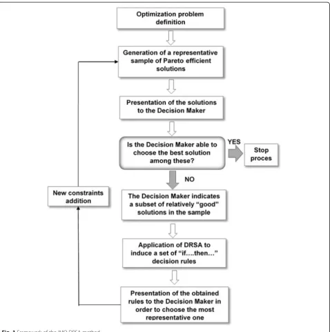
3.2.1 Framework of the method
The proposed method is innovative in that it assists the DM in the selection process. In other words, the critical assessment of the offered solutions represents a prefer-ence information useful to obtain a preferprefer-ence model of the DM, which is then used to determine a new subset of feasible solutions and to better suit the DM prefer-ences. DRSA accepts a set of exemplary decisions as in-put and in return gives a preference model in terms of easily understandable “if … , then …” decision rules explaining the exemplary decisions.
This approach can be useful in the case of an Inter-active Multiobjective Optimization procedure as pre-sented below.
Therefore, the IMO-DRSA explores the set of feasible solutions of a multiobjective optimization problem and proceeds stepwise as follow (where X is the considered set of solutions and Fi: X→R,i = 1,….,k are the object-ive functions to be maximized):
1. Generate a representative set of Pareto optimal solutions.
2. Submit such a set to the Decision Maker (DM). 3. If the DM is satisfied with one solution of the set
the procedure stops, otherwise continue. 4. Ask the DM to specify a subset of quite“good”
solutions in the sample (“good”means better that the rest in the current sample).
5. Apply DRSA to the current sample of solutions sorted into“good”and“others”, in order to induce a set of decision rules with the following syntax:“if Fi(x)≥αithen the solution is good”.
6. Submit the obtained set of rules to the DM. 7. Ask the DM to select the most representative
decision rule in the set.
8. Add the rule selected in step 7 to the set of constraints of the optimization problem at hand, in order to focus on a more interesting region of feasible solutions from the point of view of the preference of the DM.
9. Go back to step 1.
The syntax of rules induced in step 5 agrees with the maximization of objective functions. For the minimization of an objective function, the corresponding function would beFi(x)≥αi.
The constraints introduced in Step 8 are kept in the following iterations of the procedure, but they are not ir-reversible. Indeed, the DM can withdraw the set of opti-mal solutions of one of previous iterations and carry on from this point.
The framework of the IMO-DRSA method is shown in Fig.1.
3.2.2 Advantages of the proposed approach
The new method, proposed in this paper, has been intro-duced in order to overcome some of the disadvantages typical of the alternative methods.
Most of the previously listed approaches needed differ-ent input information given by the decision maker (e.g. fixing the coefficients of objectives and constraints in mathematical programming models or defining of the at-tribute weights in weighting methods).
Instead, other approaches, process the data in a way that is unclear and does not allow the decision maker to
retrieve and understand the relationship between the in-put information and the final solution. Therefore, the decision model is detected as a“black box”by the deci-sion maker.
Hence, the main difference between the proposed method and the other methods is the way in which data are introduced and processed.
The whole proposed procedure has an exploratory character. The exploration does not aim to find an objectively optimal strategy because it does not exist. As a decision aiding procedure, it facilitates explor-ation of the solution space in view of finding the best compromise strategy. This exploration is driven by preferences. The decision maker moves in this space by choosing a representative subset of the current Pa-reto frontier and by applying a rule that best fits his/ her current intentions of focusing on a more interest-ing part of the Pareto frontier.
The guidance by rules has several advantages over other preference models. As matter of fact, it is com-monly recognized that “people often prefer to make ex-emplary decisions and cannot always explain them in terms of specific parameters. For this reason, the idea of inferring preference models from exemplary decisions provided by the DM is very attractive”. [10].
The rules provide easily understandable arguments supported by pieces of preference information (decision examples) and avoid arbitrary suggestions. Moreover, the decision maker can always return to some previous point of the procedure. Step by step, the decision maker acquires deeper knowledge of the relationships between attainable values of objectives and forms his/her prefer-ences with a trial and error procedure. This interactive multiobjective optimization procedure stops when the decision maker feels convinced that the arguments in favour of a given solution that can be considered good enough to be selected.
This approach fits very well with the pavement man-agement process in which interactions among diverse stakeholders and the experts are necessary and the transparency is an important condition.
Briefly, the main features that distinguish DRSA from others methods are as follows:
Preference information is requested from decision maker merely in the form of exemplary decisions;
No prior discretization of quantitative condition attributes or criteria is necessary;
Heterogeneous data (qualitative and quantitative, ordered and no ordered, nominal and ordinal) can be treated;
The methodology is based on simple notions and mathematical tools, without using any algebraic or analytical structures.
4 Case study: The multiobjective model for optimal M&R plan
To demonstrate the applicability of IMO-DRSA, a simple example is presented. The sample road network is a large part of main road network of IX Municipality in Rome, consisting of 46 road sections, with a total length of 23 km. The starting state of the pavement network, in terms of weighted average value of performance indicators, is as follows: PCI (Pavement Condition Index) =43,3, PSI (Present Serviceability Index) =2,6, IRI (International Roughness Index) = 2,51 [m/km], average accident num-ber over a 3 years period before starting year = 29,5 [crash / year * km] (see also“snapshot”reported in Fig.2) .
Each section may be maintained with 3 mutually ex-clusive strategies (S = 3) namely Strategy 1 “do mini-mum”, Strategy 2 “functional & preservation maintenance”, Strategy 3 “structural maintenance”, which reflect the three general types of maintenance philosophies (i.e. corrective or holding maintenance, preservation or corrective maintenance, and reconstruc-tion and rehabilitareconstruc-tion maintenance). The generareconstruc-tion of candidate treatments for each strategy are made by deci-sion tree shown in Fig. 2, which are defined basing on the actual selection made by municipality. The Highway Development and Management “HDM-4” deterministic pavement performance prediction models are applied, after due calibration, to predict pavement condition, as done in many studies for urban road network [31].
The proposed model formulation considers the follow-ing data:
xi,udecision variable, which is implementation of
main-tenance strategyuth,u= 1,…s, on sectioni, (i= 1,…,n); xi,u = 1 indicates that the strategy u is applied to
sec-tion i,
xi,u = 0 indicates that the strategy u is not applied to
section i;
S set of all possible maintenance strategies u that might be applied alternatively on road sectioni,;
Ci,ucost of maintenance strategy u on sectioni;
CTOTbudget constraint in the planning period; CYEARLY yearly budget constraint in the planning period;
ci,u,ythe cost obtained applying the treatment provided by strategy u on section i in the year y of the analysis period (y = 1,…..t).
integrity of the pavement based on the distress observed on the surface of the pavement (i.e. photholes, cracking, etc.). Furthermore, the structural condition provides a convenient substitute or alternative measure of pave-ment asset value and it is used in sample formulation to quantify pavement value.
The present serviceability index “PSI” is used to characterize the contribution of the road pavement to the user comfort (ASTM E867), it is obtained from mea-surements of roughness and distress (single PIs used in the decision tree Fig.2).
Mathematically, the problem is defined as follows: Maximize:
pavement structural condition during the planning time-span
F1 xi;u
¼E¼ Xn
i¼1
Xs
u¼1
Xt
y¼1
PCIi;u;ylixi;u
L ð1Þ
user comfort during the planning time-span
F2 xi;u
¼C¼ Xn
i¼1
Xs
u¼1
Xt
y¼1
PSIi;u;yTIilixi;u
L
ð2Þ
average safety improvement during the planning time-span
F3 xi;u
¼ΔAC¼
Xn
i¼1
Xs
u¼1
Xt
y¼1
ACiCMFi;u;y
!
xi;u
" #
Lt
ð3Þ
percentage of road network in sufficient serviceability condition during the planning time-span
F4 xi;u
¼PSIS¼ Xn
i¼1
Xs
u¼1
lixi;u
Xt
y¼1
PSISi;u;y
!
Lt
ð4Þ
percentage of road network in good serviceability con-dition during the planning time-span
F5 xi;u
¼SIG¼ Xn
i¼1
Xs
u¼1
lixi;u
Xt
y¼1
PSIGi;u;y
!
Lt
ð5Þ
percentage of road network in sufficient structural condition during the planning time-span
F6 xi;u
¼PCIA¼ Xn
i¼1
Xs
u¼1
lixi;u
Xt
y¼1
PCISi;u;y
!
Lt
ð6Þ
percentage of road network in good structural condi-tion during the planning time-span
F7 xi;u
¼PCIG¼ Xn
i¼1
Xs
u¼1
lixi;u
Xt
y¼1
PCIGi;u;y
!
LT
ð7Þ
Where:
li is the length of the road section i and L¼X
i
li is
the total length of the road network;
PCIi;u;y is the annual average value of pavement
condi-tion index (ASTM D5340 standard) on the road seccondi-tion i, in the year y of the analysis period obtained applying treatment provided by strategy u;
PSIi;u;y is the annual average value ofthe Present
ser-viceability Index on section i, in the year y of the analysis period obtained applying treatment provided by strategy u;
TI is the traffic impact factor (TI = 1 if AADT≤10,000 veic/day TI = 2 if 10,000 < AADT ≤20,000 and TI = 3 if AADT> 20,000).
ACiis the expected number of accidents on site i with-out maintenance activity implementation. It is evaluated as the average accident number over a 3 years period be-fore maintenance activity implementation, assuming that the accident history before will represent the future safety performance without changes. This approach is not the most rigorous, as historical accident data suffer from the weakness of being highly variable. Because of the random nature of accidents, in the after period they may be higher or lower than in the before period even if no improvement is made (regression to the mean). The Empirical Bayes method is widely used to estimate the long term expected number of accidents in order to overcome the effects of the regression to the mean phenomenon [32–34]. However, considering the lack of appropriate data needed to use the Empirical Bayes ap-proach and also that the main topic of the paper is not safety analysis, the most simplistic method was used.
CMFi,u,y is the crash modification factor associated with the maintenance activity of strategyu on the section i in the year y; it is assumed to be a linear function of the friction index evaluated by deterioration model:
CMFi;j;y¼
0
minCMFmax;CMFmax
FIi;j;y−FImin
FIcritic−FImin
(
if FIi;j;y<FImin
FIi;j;y≥FImin
FIi,u,y is the sideway force coefficient (SFCS) on the road section i, in the year y of the analysis period, ob-tained applying treatment provided by strategy j [35].
FIcriticis the friction level (SFCS) below which the risk of accidents increases significantly (e.g. investigatory level) [36–40];
FImin is the minimum friction levels (SFCS) admitted (e.g. intervention level);
CMFmax is the maximum crash modification factor evaluated considering only the accidents correlated to the pavement condition [41–44];
PSISi,u,yis a boolean variable,PSISi,u,y= 1 indicates that
PSIi;u;y≥2:5,PSISi,u,y= 0 otherwise;
PSIGi,u,y is a boolean variable, PSIGi,u,y = 1 indicates
thatPSIi;u;y≥3:0,PSIGi,u,y= 0 otherwise;
PCIAi,u,y is a boolean variable, PCIAi,u,y = 1 indicates
thatPCIi;u;y≥20,PCIAi,u,y= 0 otherwise;
PCIGi,u,y is a boolean variable, PCIGi,u,y = 1 indicates
thatPCIi;u;y≥40,PCIAi,u,y= 0 otherwise.
Budget constraints in the planning period are intro-duced in order to ensure that the capital investment C neither exceeds the available total budget nor is at the same time too high with respect to yearly budgets. These constraints are defined as follow:
Xn
i¼1 Xs
u¼1 Xt
y¼1
ci;u;yxi;u≤CTOT and Xn
i¼1 Xs
u¼1
ci;u;yxi;u≤CYEARLY y¼1;…;t
ð8Þ
wherei= 1,…,N
in such a way that at least onexi.u,u∈S, must be equal
to 1, that is at least one maintenance strategyi must be implemented on each section.
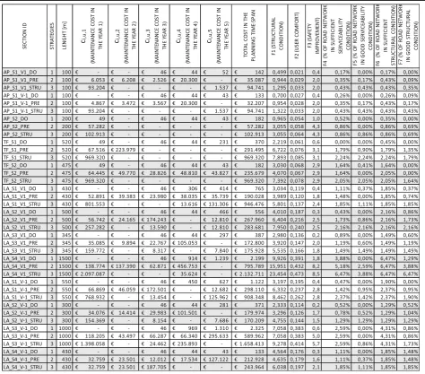
The performances (during the planning time-span) and costs (yearly and total in the planning time-span) obtained implementing the strategies considered, on some of the 46 sections of the sample, are shown in Table1, for the sake of example only. The description of the strategies 1, 2 and 3 is reported in Fig. 2. As the three strategies generated for each sections are mutually exclusive, the DM will have to choose which of these to implement on each section in order to optimize the con-sidered objective functions, within budget constraints.
A set of Pareto optimal solutions is found and submitted to the DM. Since the considered problem is a Multiple Objective Linear Programming, the Pareto optimal solu-tions are found using classical linear programming,.
In this problem, the variables are xi,u, u= 1, …,s, i= 1,
The objective functions and the constraints considered in the optimization problem are those defined previously in expressions defined by items (1) to (8).
In the presented example the budget constraints are:
CTOT≤4:034:300€ and CYEARLY≤1:049:000€
Within the total budget, the annual budget may be dif-ferent year by year (± 30% of the average annual budget) in order to guarantee a minimum spending flexibility from year to year.
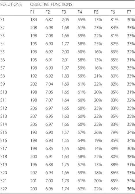
A set of 22 Pareto optimal solutions was found, main-taining the fixed budget constraints and then maximiz-ing Fkunder the constraint of attaining some targets on the other objective functions (see Table2).
Each solution reported in Table 2 corresponds to a combination of countermeasures (generated by the im-plementation of a strategy) to be implemented in the road sections of the considered sample and, from among these, the DM was not able to choose the best solution to be implemented.
5 Results and discussion about application of IMO-DRSA to the case study
To refine the search for more satisfying solutions, the DRSA was used to induce decision rules from the DM’s preferences (for more details about the method see [8– 10]). For this aim, the DM was requested to indicate, among the proposed solutions in Table2, a subset of (rela-tively)“good”solutions, which are reported in the“ evalu-ation” column of the same table. In this case, the DM selected the solutions S5, S6, S7, S21 and S22 as“good”.
Taking into account the sorting by the DM of Pareto optimal solutions into“good”and “others”, five decision rules were induced from the lower approximation of
“good”solutions.
The following are the most supported induced rules (the identification numbers of solutions supporting the rule are in parenthesis):
rule1)if the user comfort (F2) is at least 6,9 and the safety improvement (F3) is at least 1,97, then the solution is good; (S5, S6, S7)
rule 2)if the structural condition (F1) is at least 193 and the safety improvement (F3) is at least 2, then the solution is good; (S5, S6)
rule 3)if the percentage of road network in acceptable structural condition (F6) is at least 83% and the safety improvement (F3) is at least 2, then the solution is good; (S5, S6)
rule 4)if the percentage of road network in acceptable serviceability condition (F4) is at least 59% and the safety improvement (F3) is at least 1,97, then the solution is good; (S5, S7)
rule 5)if the percentage of road network in good serviceability condition (F5) is at least 16% and the safety improvement (F3) is at least 1,97, then the solution is good; (S5, S7)
rule 6)if the percentage of road network in acceptable structural condition (F6) is at least 82% and the safety improvement (F3) is at least 1,97, then the solution is good; (S5, S6, S7)
rule 7)if the percentage of road network in acceptable serviceability condition (F2) is at least 61% and the safety improvement (F3) is at least 1,73, then the solution is good; (S21, S22)
rule 8)if the percentage of road network in good structural condition (F7) is at least 34% and the safety improvement (F3) is at least 1,73, then the solution is good; (S7, S21, S22).
These rules were presented to the DM and he was re-quested to select the most representative based on own preferences. The DM selected rule 6) and this rule per-mitted the definition of the following constraint thereby reducing the feasible region of the problem:
F3 (safety improvement) > 1,97
F6 (percentage of road network in acceptable struc-tural condition) > 82%
These new constraints were used together with the original constraints in order to update the Pareto fron-tier zone interesting from the point of view of DM’s preferences. At this point, a new multiobjective model with the addition of the new constraints was constructed and a new set of efficient solutions was induced by means of another process analogous to the first one. From the so restricted efficient frontier, five solutions were selected to be presented to the DM (see Table3).
The DM was asked again if he was satisfied with one of the proposed Pareto optimal solutions.
In general, two scenarios are possible:
1) The DM is satisfied with one of the presented Pareto optimal solutions and this ends the interactive procedure.
2) The DM is not satisfied with any of the presented Pareto optimal solutions and, in this case, the
Table 2Sample of Pareto optimal solutions proposed in the
first interaction
SOLUTIONS OBJECTIVE FUNCTIONS
F1 F2 F3 F4 F5 F6 F7
S1 184 6,87 2,05 55% 13% 81% 30%
S2 208 6,98 1,68 61% 23% 84% 35%
S3 198 7,08 1,66 59% 22% 81% 33%
S4 195 6,90 1,77 58% 25% 82% 33%
S5 193 6,92 2,00 60% 16% 83% 32%
S6 195 6,91 2,01 58% 13% 85% 31%
S7 198 6,90 1,97 59% 16% 82% 35%
S8 192 6,92 1,83 59% 21% 80% 33%
S9 202 7,04 1,69 61% 22% 82% 35%
S10 198 7,05 1,66 61% 20% 85% 31%
S11 198 7,07 1,64 60% 20% 83% 32%
S12 206 6,97 1,65 60% 25% 83% 35%
S13 207 6,95 1,63 60% 22% 85% 35%
S14 206 6,97 1,66 60% 25% 83% 35%
S15 193 6,90 1,57 57% 26% 79% 34%
S16 198 6,93 1,55 64% 19% 85% 34%
S17 198 6,85 1,55 60% 14% 89% 30%
S18 200 6,91 1,63 58% 22% 80% 38%
S19 196 6,88 1,75 57% 13% 88% 31%
S20 202 6,94 1,66 59% 18% 86% 33%
S21 201 7,00 1,73 61% 20% 85% 34%
S22 200 6,96 1,74 62% 22% 84% 36%
Table 3Sample of Pareto optimal solutions proposed in the
second interaction
SOLUTIONS OBJECTIVE FUNCTIONS
F1 F2 F3 F4 F5 F6 F7
S1’ 200 6,90 226 58% 15% 84% 33%
S2’ 199 6,96 227 59% 16% 84% 33%
S3’ 191 7,01 226 58% 17% 82% 31%
S4’ 196 6,93 227 60% 16% 84% 34%
interactive procedure must be reapplied until the DM is satisfied with one of the presented solutions.
In our case study, the DM was satisfied with S2’, so the interactive procedure was concluded.
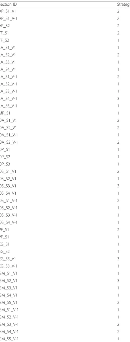
The strategies to be implemented on each section ac-cording to the solution S2’ is shown in Table4 and the resulting optimum budget for each year of the analysis period is shown in Table5.
To induce the decision rules a tool, called jMAF, was used. In this tool an algorithm based on the DRSA methodology is implemented and it is available free of charge in the web. The computational time was less than 1 ms, in the case study and, as stated by Augeri et al., it should be less than 4 s for larger information table (e.g. 1400 objects and 16 attributes) [45].
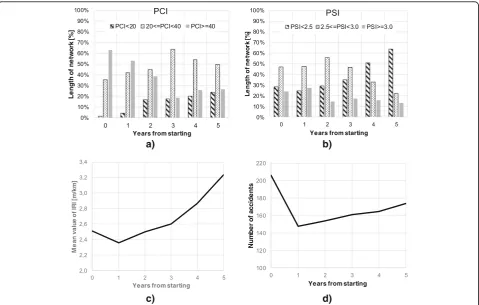
An overview of the pavement network starting and fu-ture performances is given in Fig.3, where detailed data of PCI and PSI indicators are aggregated in three classes (as in the objective functions) and reported next to the mean values roughness and number of crashes related to pavement condition. Despite all the optimization work, the figure clearly indicates a generally worsening of structural and serviceability condition and an improve-ment of safety in the example network. The results are a consequence of the sensitivity the decision maker have to safety issues, and, above all, of the small budget in the example. As far as the budget is concerned, the real meagre economic resource destined to road pavement maintenance by municipality was considered an excel-lent opportunity for checking the method in very strict condition.
The results obtained shows that IMO-DRSA is a useful tool to reduce the Pareto optimal set in multiobjective optimization problems, allowing the DM to select the best solution among a large number of feasible solutions. The proposed method is based on a decision rule prefer-ence model that gives argumentation for preferprefer-ences in a logical form and, therefore, is understandable for the DM. Although a small subset of road sections was used to demonstration purposes, the method can also be ap-plied to practical application involving a larger subset of sections.
6 Conclusion
In this paper, a methodology for pavement management and optimal allocation of funds is presented. For this pur-pose, an interactive optimization method using a decision-rule preference model (IMO-DRSA) was used to support interaction with the DM. With regard to the meth-odological procedure, any multiobjective optimization method that finds the Pareto optimal set, or its approxima-tion, is generally well complemented by the IMO-DRSA.
Table 4Strategies to be implemented on each section for
preferred solution S2
Section ID Strategy
AP_S1_V1 2
AP_S1_V-1 2
AP_S2 2
TF_S1 2
TF_S2 1
LA_S1_V1 1
LA_S2_V1 2
LA_S3_V1 1
LA_S4_V1 1
LA_S1_V-1 2
LA_S2_V-1 1
LA_S3_V-1 1
LA_S4_V-1 3
LA_S5_V-1 1
MP_S1 1
OA_S1_V1 2
OA_S2_V1 2
OA_S1_V-1 1
OA_S2_V-1 2
OP_S1 1
OP_S2 1
OP_S3 1
OS_S1_V1 2
OS_S2_V1 1
OS_S3_V1 3
OS_S4_V1 1
OS_S1_V-1 2
OS_S2_V-1 1
OS_S3_V-1 1
OS_S4_V-1 1
PF_S1 2
VF_S1 1
EG_S1 1
EG_S2 1
EG_S3_V1 3
EG_S3_V-1 1
GM_S1_V1 1
GM_S2_V1 3
GM_S3_V1 1
GM_S4_V1 1
GM_S5_V1 2
GM_S1_V-1 1
GM_S2_V-1 1
GM_S3_V-1 2
GM_S4_V-1 2
In fact, one of the biggest difficulties in a prioritization problem is the large number of the feasible solutions, which makes it hard for the DM to select the best solu-tion. Therefore, the strong point of the proposed method is to provide a tool that helps him or her in this step of the decision process.
As for the input, the DM gives preference information by answering easy questions about the sorting of some representative solutions into two classes (“good” and
“others”). The output is a model of preferences in terms of “if …, then …” decision rules, which is then used to reduce the Pareto optimal set iteratively until the DM selects a satisfactory solution.
The transparency and intelligibility in the transform-ation of the input informtransform-ation into the preference model allows us to consider the proposed method as a “glass box”, contrary to the “black box” effect typical of many methods that give a result without any clear explanation. This is because the decision rules explain the final deci-sion, which is not the result of a simple application of a
technical method, but rather, is derived from a decision process based on the active participation of the DM.
The decision rule preference model is very convenient for decision support because it gives argumentation for preferences in a logical form and, therefore, is intelligible for the DM.
Decision rules provide a well understandable link be-tween the calculation stage and the decision stage. Due to this feature, the final decision does not arise from an automatic application of a method, but rather from the conclusion of a decision process based on active partici-pation of the DM.
Unlike any method including scalarization, the sug-gested technique does not require to aggregate the ob-jectives, avoiding operations such as averaging, weighted sum, different types of distance, which always derive from subjective judgments. Indeed, the IMO-DRSA works on data using only ordinal comparisons, which would not be affected by any increasing monotonic transformation of scales, and this ensures the meaning-fulness of results from the point of view of measurement theory.
With the aim of demonstrating the strength of the method, an application on a sample of road pavements of an Italian urban sub-network, considering a number
a) b)
c) d)
Fig. 3Summary of pavement performance over the analysis period for the solution S2’: distribution of the network in the classes of PCI and PSI (aandb), average roughness (c) and yearly frequency of crashes correlated to the pavement condition (d)
Table 5Yearly budget for solution S2
Budget year 1 Budget year 2 Budget year 3 Budget year 4 Budget year 5
of mutually exclusive strategies at each section, is presented.
A five-year analysis period is considered, but the pro-posed model is generic and scalable with flexibility in in-cluding different types of maintenance strategies, planning periods, policy options and budget (yearly or overall).
The case study application has shown the suitability of the IMO-DRSA methodology in order to identify the best combination of maintenance actions given budget constraints.
Abbreviations
CB:Cost-benefit; CE: Cost-effectiveness; DM: Decision Maker; DSE: Decision support element; IMO-DRSA: Interactive Multiobjective Optimization-Dominance Rough Set Approach; IRI: International Roughness Index; M&R: Maintenance and rehabilitation; MOO: Multiobjective optimization; PCI: Pavement Condition Index; PMS: Pavement management systems; PSI: Present Serviceability Index
Acknowledgements
Not applicable.
Funding
Not applicable.
Availability of data and materials
The datasets used in the study are available from the corresponding author on reasonable request. To induce the decision rules a tool, called jMAF, was used. It is available free of charge in the web.
Authors’contributions
SG carried out and applied the new interactive multiobjective optimization method. MGA and VN designed the study and carried out the experimental application. All authors read and approved the final manuscript.
Competing interests
The authors declare that they have no competing interest.
Publisher’s Note
Springer Nature remains neutral with regard to jurisdictional claims in published maps and institutional affiliations.
Author details
1Department of Enterprise Engineering, University of Rome“Tor Vergata”, Via
del Politecnico 1, 00133 Rome, Italy.2Department of Economics and
Quantitative Methods, University of Catania, Corso Italia 55, 95129 Catania, Italy.3Portsmouth Business School, Centre of Operations Research and
Logistics (CORL), University of Portsmouth, Portsmouth, UK.
Received: 14 September 2018 Accepted: 19 February 2019
References
1. Bruun M (2013). Social benefit report (ERANET). Joint research collaborations ERA-NET ROAD and CEDR, http://http://www.cedr.eu/download/other_ public_files/research_programme/eranet_road/call_2010_asset_ management/end_of_programme_report/2013-Asset-management-Social-benefit-report.pdf(ISBN: 9788770607568, 9788770607551 digital). 2. Benchmarking of expenditures and practices of maintenance and opera
Report (BEXPRAC), 2010. Conference of European directors of roads (CEDR), Paris.
3. Wu, Z., Flintsch, G., Ferreira, A., & Picado-Santos, L. (2012). Framework for multiobjective optimization of physical highway assets investments.J Transp Eng, 138(12), 1411–1421.
4. Highway Infrastructure Asset Management Guidance Document (HMEP). (2013).Maintenance efficiency Programme. London: Queen’s Printer and
Controller of Her Majesty’s Stationery Officehttp://www. ukroadsliaisongroup.org/download.cfm/docid/5C49F48E-1CE0-477F-933ACBFA169AF8CB.
5. Dekker, R., & Scarf, P. A. (1998). On the impact of optimisation models in maintenance decision making: The state of the art.Reliability Engineering & System Safety, 60(2), 111–119.
6. Marler, R. T., & Arora, J. S. (2004). Survey of multi-objective optimization methods for engineering.Struct Multidiscip Optim, 26(6), 369–395. 7. Pareto V (1906). Manuale di Economica Politica, Società Editrice Libraria.
Milan; translated into English by A.S. Schwier as Manual of Political Economy, edited by A.S. Schwier and A.N. Page (1971). New York: A.M. Kelley.
8. Greco, S., Matarazzo, B., & Slowinski, R. (2001). Rough sets theory for multicriteria decision analysis.Eur J Oper Res, 129, 1–47.
9. Greco, S., Matarazzo, B., & Slowinski, R. (2005). Decision rule approach. In J. Figueira, S. Greco, & M. Ehrgott (Eds.),Multiple criteria decision analysis: State of the art surveys(pp. 507–555). New York: Springer-Verlag.
10. Branke, J., Branke, J., Deb, K., Miettinen, K., & Slowiński, R. (Eds.). (2008). Multiobjective optimization: Interactive and evolutionary approaches (Vol. 5252). Springer Science & Business Media.
11. Kabir, G., Sadiq, R., & Tesfamariam, S. (2014). A review of multi-criteria decision-making methods for infrastructure management.Struct Infrastruct Eng, 10(9), 1176–1210.
12. Dissanayake, S., Lu, J. J., Chu, X., & Turner, P. (1999). Use of multicriteria decision making to identify the critical highway safety needs of special population groups.Transportation Research Record, 1693, 13–17.
13. Lambert, J. H., Wu, Y. J., You, H., Clarens, A., & Smith, B. (2012). Future climate change and priority setting for transportation infrastructure assets.ASCE J Infrastruct Syst.https://doi.org/10.1061/(ASCE)IS.1943-555X.0000094. 14. Gharaibeh, N., Chiu, Y., & Gurian, P. (2006). Decision methodology for
allocating funds across transportation infrastructure assets.J Infrastruct Syst, 12(1), 1–9.
15. Li, Z., & Sinha, K. C. (2004). Methodology for multicriteria decision making in highway asset management.Transportation Research Record, 1885, 79–87. 16. Selih, J., Kne, A., Srdic, A., & Zura, M. (2008). Multiple-criteria decision support
system in highway infrastructure management.Transport, 23(4), 299–305. 17. Shelton, J., & Medina, M. (2010). Integrated multiple-criteria decision-making
method to prioritize transportation projects.Transp Res Rec, 2174, 51–57. 18. Farhan, J., & Fwa, T. F. (2009). Pavement maintenance prioritization using
analytic hierarchy process.Transp Res Rec, 2093, 12–24.
19. Sun, L., & Gu, W. (2011). Pavement condition assessment using fuzzy logic theory and analytic hierarchy process.J Transp Eng.https://doi.org/10.1061/ (ASCE)TE.1943-5436.0000239.
20. Chou, S. Y., Chang, Y. H., & Shen, C. Y. (2008). A fuzzy simple additive weighting system under group decision-making for facility location selection with objective/subjective attributes.Eur J Oper Res, 189(1), 132–145.
21. Pilson, C., Hudson, W. R., & Anderson, V. (1999). Multiobjective optimization in pavement management by using genetic algorithms and efficient surfaces.Transportation Research Record, 1655(1), 42–48.
22. Fwa, T., Chan, W., & Hoque, K. (2000). Multiobjective optimization for pavement maintenance programming.J Transp Eng.https://doi.org/10.1061/ (ASCE)0733-947X(2000)126:5(367.
23. Chan, W. T., Fwa, T. F., & Tan, J. Y. (2003). Optimal fund-allocation analysis for multidistrict highway agencies.Journal of Infrastructure System.https://doi. org/10.1061/(ASCE)1076-0342(2003)9:4(167.
24. Chootinan, P., Chen, A., Horrocks, M. R., & Bolling, D. (2006). A multi-year pavement maintenance program using a stochastic simulation-based genetic algorithm approach.Transp Res A Policy Pract, 40(9), 725–743. 25. Morcous, G., & Lounis, Z. (2005). Maintenance optimization of infrastructure
networks using genetic algorithms.Autom Constr, 14(1), 129–142. 26. Mathew, B. S., & Isaac, K. P. (2014). Optimisation of maintenance strategy for
rural road network using genetic algorithm.International Journal of Pavement Engineering, 15(4), 352–360.
27. Elhadidy, A. A., Elbeltagi, E. E., & Ammar, M. A. (2015). Optimum analysis of pavement maintenance using multi-objective genetic algorithms.HBRC Journal, 11(1), 107–113.
28. Santos, J., Ferreira, A., & Flintsch, G. (2017). An adaptive hybrid genetic algorithm for pavement management.International Journal of Pavement Engineering.https://doi.org/10.1080/10298436.2017.1293260.
Miettinen, & R. Slowiski (Eds.),Multiobjective optimization: Interactive and evolutionary approaches(pp. 121–155). Berlin: Springer-Verlag. 30. Cohon, J. L. (1985).Multicriteria programming: Brief review and application.
New York, NY: Academic Press.
31. Jorge, D., & Ferreira, A. (2012). Road network pavement maintenance optimisation using the HDM-4 pavement performance prediction models. International Journal of Pavement Engineering, 13(1), 39–51.
32. Elvik, R. (2008). The predictive validity of empirical Bayes estimates of road safety.Accid Anal Prev, 40(6), 1964–1969.
33. Hauer, E. (1997).Observational Before–After Studies in Road Safety: Estimating the Effect of Highway and Traffic Engineering Measures on Road Safety. Oxford: Pergamon Press, Elsevier Science Ltd..
34. Hauer, E., Harwood, D. W., & Griffith, M. S. (2002).Estimating safety by the empirical Bayes method: A tutorial, transportation research record, 1784(pp. 126–131). Washington, D. C: National Research Council, Transportation Research Board.
35. CEN/TS5901–6. (2009). Road and airfield surface characteristics. InProcedure for determining the skid resistance of a pavement surface by measurement of the sideway force coefficient (SFCS)SCRIM (ISBN 978 0 580 67241 5). 36. Bullas J C (2004). Tyres, road surfaces and reducing accidents-a review.
Report prepared for AA Foundation, United Kingdom.
37. Erwin, T., & Tighe, S. (2008). Safety effect of preventive maintenance: A case study of microsurfacing.Transportation Research Record: Journal of the Transportation Research Board, 2044, 79–85.
38. Gothié, M. (2000). Apport à la sécurité routière des caractéristiques de surface des chaussées.Bulletin des laboratoires des Ponts et Chaussées, 224, 5–11.
39. Larson, R. M., & Smith, K. L. (2010).Relationship between pavement surface characteristics and crashes, Volume 1: Synthesis Report.
40. Wallman CG, Åström H (2001). Friction measurement methods and the correlation between road friction and traffic safety: A literature review. Statens väg-och transportforskningsinstitut.
41. Smith KL, Larson R. (2011). Engineering Safer Road Surfaces to Help Achieve US Highway Safety Goal. Proc.3rd International Conference on Road Safety and Simulation.
42. Shen J, Rodriguez A, Gan A, Brady P (2004). Development and application of crash reduction factors: a state-of-the-practice survey of State Departments of Transportation, Proc., 83th Transportation Research Board Annual Meeting.
43. ARRB (Australian Road Research Board) (2012). Austroads Road Safety Engineering Toolkit.
44. FHWA (Federal Highway Administration) (2013). Crash modification factors clearinghouse. Retrieved fromhttp://www.cmfclearinghouse.org/ 45. Augeri, M. G., Colombrita, R., Greco, S., Lo Certo, A., Matarazzo, B., &