R E S E A R C H
Open Access
A variant of the Hough Transform for the
combined detection of corners, segments,
and polylines
Pilar Bachiller-Burgos
*, Luis J. Manso and Pablo Bustos
Abstract
The Hough Transform (HT) is an effective and popular technique for detecting image features such as lines and curves. From its standard form, numerous variants have emerged with the objective, in many cases, of extending the kind of image features that could be detected. Particularly, corner and line segment detection using HT has been separately addressed by several approaches. To deal with the combined detection of both image features (corners and segments), this paper presents a new variant of the Hough Transform. The proposed method provides an accurate detection of segment endpoints, even if they do not correspond to intersection points between line segments. Segments are detected from their endpoints, producing not only a set of isolated segments but also a collection of polylines. This provides a direct representation of the polygonal contours of the image despite imperfections in the input data such as missing or noisy feature points. It is also shown how this proposal can be extended to detect predefined polygonal shapes. The paper describes in detail every stage of the proposed method and includes experimental results obtained from real images showing the benefits of the proposal in comparison with other approaches.
Keywords: Hough Transform, Corner detection, Line segment detection, Polyline detection
1 Introduction
Corner and line segment detection is essential for many computer vision applications. Corner detection is used in a wide variety of applications such as camera calibration [1], target tracking [2], image stitching [3], and 3D model-ing [4]. The detection of line segments can also be helpful in several problems including robot navigation [5], stereo analysis [6], and image compression [7]. Going a step fur-ther, the combined detection of both image features may result in the identification of polygonal structures, which plays an important role in many applications such as aerial imagery analysis [8, 9] and cryo-electron microscopy [10]. The Hough Transform (HT) [11] is one of the most popular and widely used techniques for detecting image features such as lines, circles, and ellipses [12]. Its effec-tiveness emerges from its tolerance to gaps in feature boundaries and its robustness against image noise. These
*Correspondence: [email protected]
Department of Computer and Communication Technology, University of Extremadura, Avda. de la Universidad s.n., 10003 Caceres, Spain
properties make HT a powerful tool for detecting image features in real images. To exploit its benefits, we propose a new variant of the HT, called HT3D, for the combined detection of corners and line segments.
The basic form of the Hough Transform, also known as the Standard Hough Transform (SHT) [13], has been established as the main technique for straight line detec-tion [14–16]. The line detecdetec-tion problem is transformed by the SHT into a peak detection problem. Each feature point, obtained from a previous pre-processing stage such as edge detection, is mapped to a sine curve following the expression d = xcos(θ)+ ysin(θ). The parameter space defined by(θ,d)is discretized into finite intervals, called accumulator cells or bins, giving rise to the Hough space (also referred to as the accumulator array). Using this discrete version of the parameter space, each feature point votes for the lines passing through it by increment-ing the accumulator cells that lie along the correspondincrement-ing curve. After this voting process, lines are located at those positions forming local maxima in the Hough space.
The SHT for straight line detection does not provide a direct representation of line segments, since feature points are mapped to infinite lines in the parameter space. To deal with segment representation, we propose a 3D Hough space that, unlike SHT, uses several bins to represent each line. This 3D Hough space not only provides a segment representation but also encloses canonical configurations of two kinds of distinctive points: corners and non-intersection endpoints. Corners are points at which two line segments meet at a particular angle. Non-intersection endpoints are extreme points of line segments that do not intersect any other segment. Both types of points iden-tify line segment boundaries, but corners can additionally be considered connection points among segments. This makes it possible to extend line segment detection to the identification of chains of segments. Thus, the pro-posed parameter space constitutes a suitable structure for detecting three kinds of image features: corners, line segments, and polylines.
The use of HT for individual detection of corners and line segments has been explored from different approaches over the last few decades.
For segment detection, two main approaches have been proposed. The first group of methods is based on image space verification from the information of the HT peaks. Song and Lyu [17] propose an HT-based segment detec-tion method which utilizes both the parameter space and the image space. Using a boundary recorder for each parameter cell, the authors develop an image-based line verification algorithm. The boundary recorder of each cell includes the upper and lower boundaries which enclose all feature points contributing to that cell. Gerig [18] sug-gests a backmapping which links the image space and the parameter space. After the accumulation phase, the transform is used a second time to compute the loca-tion of the cell most likely to be related to each image point. This backmapping process provides a connection between edge points and Hough cells in the detection of line segments. Matas et al. [19] present PPHT (Progressive Probabilistic Hough Transform), a Monte Carlo variant of the Hough Transform. PPHT obtains line segments by looking along a corridor in the image specified by the peak in the accumulator modified during pixel voting. Nguyen et al. [20] propose a similar strategy, but in this approach, the method is based on SHT with some extensions.
The other group of methods for segment detection detects properties of segments by analyzing the data in the parameter space. Cha et al. [21] propose an extended Hough Transform, where the Hough space is formed by 2D planes that collect the evidence of the line segment that passes through a specific column of the input image. Using this scheme, a feature extraction method is pro-posed for detecting the length of a line segment. In the study by Du et al. [22], the authors propose a segment
detection method based on the definition and analysis of the neighborhoods of straight line segments in the param-eter space. In another study [23], the paramparam-eters of a line segment are obtained by analyzing the distinct distribu-tion around a peak in the accumulator array. This distri-bution is called butterfly distridistri-bution due to its particular appearance. Xu and Shin [24] propose an improvement of the peak detection by considering voting values as prob-abilistic distributions and using entropies to estimate the peak parameters. Endpoint coordinates of a line segment are then computed by fitting a sine curve around the peak. In relation to corner detection using HT, various meth-ods can be found in the literature. Davies [25] uses the Generalized Hough Transform [26] to transform each edge pixel into a line segment. Corners are found at peaks in the Hough space, where lines intersect. Barret and Petersen [27] propose a method to identify line intersec-tion points by finding collecintersec-tions of peaks in the Hough space through which a given sinusoid passes. Shen and Wang [28] present a corner identification method based on the detection of straight lines passing through the ori-gin in a local coordinate system. For detecting such lines, the authors propose a 1D Hough Transform.
Unlike other methods, our proposal provides an inte-grated detection of corners and line segments, which has important benefits in terms of accuracy and applicability of the results. Thus, segments are detected from pre-viously extracted endpoints, which guarantees a better correspondence between detected and actual segments than other approaches. Corners are detected by search-ing for points intersectsearch-ing two line segments at a given range of angles. This makes it possible to detect features that other methods miss, such as obtuse-angle corners. Besides corners, our technique detects the location of any segment endpoint with high accuracy, even if such an end-point does not belong to any other segment. In addition, the proposed method produces chains of segments as a result of segment detection, providing a complete repre-sentation of the polygonal contours of the image despite imperfections in the input data such as missing or noisy feature points.
with real images, comparing the methods proposed in this paper with other approaches. Finally, Section 4 summa-rizes the main conclusions of this paper.
2 The proposed method
2.1 The 3D Hough space
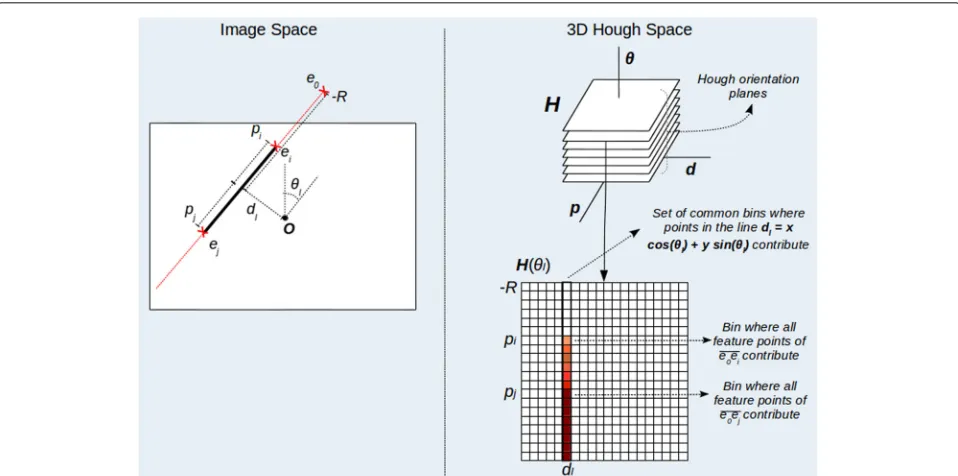
To deal with the detection of line segments using HT, a parametrization of the geometric model of this kind of image features must be established. Thus, assume that two pointsei = (xi,yi)andej = (xj,yj)define an image segment of the line l(d,θ) ≡ d = xcos(θ)+ ysin(θ). Letpi andpjbe the positions ofei andejrelative to the linel(d,θ). To compute these relative positions, consider a coordinate system local to the line where the vertical axis coincides with the line and the horizontal one passes through the image origin (see Fig. 1). Using this local sys-tem, the relative position (p) of a pointe=(x,y)of the line l(d,θ)can be computed by determining they-coordinate of the point as follows:
p= −xsin(θ)+ycos(θ) (1)
According to this and takingpi < pj, a pointe =(x,y) belongs to the segmenteiejif it fulfills the following two expressions:
d = xcos(θ)+ysin(θ) (2)
pj> = −xsin(θ)+ycos(θ) >=pi (3)
Equation 2 determines whether the pointebelongs to the line l(d,θ). The additional condition expressed by Eq. 3 forces the pointeto be situated betweeneiandej.
Considering the conditions imposed by these two expressions, a line segment can be described by four parameters:d,θ,pi, andpj. It is assumed that the origin of the image coordinate system is located at its center. Thus,
Fig. 1Relative positionpof an image pointeto the linel(d,θ). The relative positionpis computed by determining they-coordinateof the pointein a coordinate system local to the linel(dotted red lines). It is considered that the image reference system (dotted blue lines) is situated at the image center (O)
θ ∈[0,π), andd,pi,pj∈[−R,+R], withRbeing the half of the length of the image diagonal. This leads to a 4D param-eter space, where each feature point(x,y) in the image contributes to those points(θ,d,pi,pj)of the parameter space that verify Eqs. 2 and 3.
This parameter space provides a complete representa-tion of image line segments. Nevertheless, in practice, the use of a 4D structure could make the detection method excessively demanding in terms of memory and time. To tackle this problem, a 3D parameter space representing a subset of line segments is proposed (Fig. 2). This seg-ment subset is defined by the point pairse0−ej, withe0
being a fixed endpoint situated at the smallest line posi-tion(p0= −R)andeja variable endpoint situated at any positionpwithin a line. Thus, the proposed Hough space is parametrized by (θ,d,p), withθanddbeing the param-eters of the line representation (l(d,θ)≡ d =xcos(θ)+ ysin(θ)) as in the standard HT. The additional parame-terpdefines the relative position ofejfor a given segment e0ejof the linel(d,θ). Using this representation, any point (x,y) contributes to those points (θ,d,p) in the Hough space verifying Eq. 2 and the expression of Eq. 3, taking pias−Randpj asp. Since the parameterpranges from −RtoR, the last inequation of expression 3 is always true. Thus, such an expression can be rewritten as follows:
p>= −xsin(θ)+ycos(θ) (4)
Although this 3D Hough space does not directly rep-resent every possible segment of the image, it allows computing the total number of points included in any given segment (see Fig. 2). For instance, take a segment of a given linel(dl,θl)defined by the endpointsei =(xi,yi) andej = (xj,yj). Assuming that, for the linel,pi is lower thanpj, it can be stated that segmente0ei is included in e0ej. Thus, the number of points belonging toeiej, which is denoted byHi↔j, can be computed as:
Hi↔j= |H(θl,dl,pi)−H(θl,dl,pj)| (5)
withHbeing the proposed 3D Hough space.
This last equation leads into the quantification of the segment strength, which for two points ei andej can be expressed as:
ss(ei,ej)=Hi↔j/
(xi−xj)2+(yi−yj)2 (6) The values ofss(ei,ej)range from 0 to 1. The higher the value, the higher the likelihood of the existence of a line segment betweeneiandej.
2.1.1 The voting process
Fig. 23D Hough space and line segment representation. Points of a linel(dl,θl)contribute to a subset of cells situated atdlin the Hough plane H(θl). Specifically, a pointeisituated at a positionpirelative to the linel(dl,θl)contributes to the subset of cells for whichp>=pi. As a
conse-quence, the binH(θl,dl,pi)contains the total number of feature points of the segmente0ei. Likewise, the binH(θl,dl,pj)contains the number of
feature points ofe0ej. Thus, the difference between the contents of both bins provides the total number of feature points of the segmenteiej
and 4. This process is computationally expensive, since it entails running two nested loops for every feature point. However, this complexity can be reduced by dividing the voting process into two stages: (a) points only vote for the first segment they could belong to in every orienta-tion plane, i.e.,pis computed using only the equality of expression 4; (b) starting from the second discrete value of p (pd = pmin + 1), each cell in H(θd,dd,pd) accu-mulates with H(θd,dd,pd − 1) forθd ∈[θmin,θmax] and dd ∈[dmin,dmax]. Algorithms 1 and 2 describe these two stages. As it can be observed, in the second stage, each cell inHis saturated topbefore accumulation takes place. Cell saturation means that every cell crossed by a segment must contain a minimum contribution for it to be con-sidered an actual segment. This reduces false positives in the detection of segments caused by the contribution of different line points to common bins.
To improve the efficiency of this voting scheme, addi-tional optimizations can be introduced. Thus, as sug-gested in some approaches, the local orientation of the edges can be used to limit the range of angles over which a point should vote [26]. This reduces the computational cost of Algorithm 1. In relation to Algorithm 2, a possible optimization consists of storing, for every line, the mini-mum value ofpd for which points have voted and using this value to start each accumulation loop. This means that if a line of the Hough space has no points, it will not be taken into account at the accumulation stage, and so the time needed to execute that stage is reduced.
Algorithm 1First stage of the voting process 1: foreach edge point(x,y)do
2: forθd=θmin. . .θmaxdo
3: Compute the real valueθassociated toθd 4: Computed=xcos(θ)+ysin(θ)
5: Compute the discrete valueddassociated tod 6: Computep= −xsin(θ)+ycos(θ)
7: Compute the discrete valuepdassociated top 8: IncrementH(θd,dd,pd)by 1
9: end for
10: end for
Algorithm 2Second stage of the voting process 1: forθd=θmin. . .θmaxdo
2: fordd=dmin. . .dmaxdo 3: ifH(θd,dd,pmin) > pthen 4: H(θd,dd,pmin)←p
5: end if
6: forpd=pmin+1 . . .pmaxdo 7: ifH(θd,dd,pd) > pthen 8: H(θd,dd,pd)←p
9: end if
10: H(θd,dd,pd)←H(θd,dd,pd)+H(θd,dd,pd−1)
11: end for
12: end for
Fig. 3Representation of two segments of a linel(dl,θl)in the 3D Hough space
2.1.2 Interpreting the 3D Hough space
Using the proposed parameter space, segment detection cannot be treated as a traditional peak detection prob-lem, since each cell only contains information about one of the two endpoints of a given segment. Complete segment parametrization is held in pairs of cells with common values of θ and d. Thus, segment detection is accom-plished by searching for pairs of cells belonging to the same line that exhibit a ratio of close to 1 between the difference of content (number of points included between segment endpoints) and the difference of position (seg-ment length). To avoid detecting seg(seg-ment parts as inde-pendent segments, it is required that a line segment may not belong to a longest segment. Figure 3 shows this idea. This figure graphically depicts the content of the cells associated with a given linel(dl,θl) using a continuous function in parameter space for simplification. The evolu-tion of cell contents shows the existence of two (ideal) line segments: the first one situated between line positionspi andpjand the other one betweenpkandpl.
This strategy for segment detection presents two main drawbacks. Firstly, the computational cost of checking the segment feature for every pair of cells of each line is excessive. In addition, in the discrete parameter space, the accuracy of segment representation could not be enough to obtain useful results. To solve both problems, we pro-pose detecting segment endpoints instead of complete segments and using the resulting positions to confirm the existence of line segments. The benefit of applying this process is twofold: in the first place, segment end-points can be detected from local cell patterns, reduc-ing considerably the cost of feature detection; secondly, starting from the initial positions of points detected in the parameter space, segment endpoints can be accu-rately located in the image space computing the pixel
locations that maximize an endpoint measure in a local environment.
The following subsections describe this approach to fea-ture detection. Starting from segment endpoints detection (Subsection 2.2), it is detailed how to extract line seg-ments from the 3D Hough space with good precision (Subsection 2.3) as well as more complex image features (Subsection 2.5).
2.2 Detection of segment endpoints
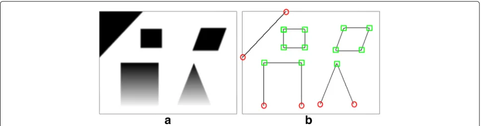
In our proposal, segment endpoints are classified into two types of distinctive points: corners and non-intersection endpoints. A corner point is a point that belongs to at least two segments. A non-intersection endpoint is an extreme point of a segment which does not belong to any other segment. Figure 4 shows some representative examples of both kinds of points.
Fig. 4Examples of the different kinds of line segment endpoints considered in the proposed detection method.aOriginalgrayimage.bLine segments obtained by an edge detection process. In this second image, corners are marked withgreen squaresand non-intersection endpoints with
red circles. Corners correspond to the crossing points of two line segments at a certain range of angles. Non-intersection endpoints appear in the intersections of line segments with the image boundaries as well as in the start and end points of the open polylines resulting from image areas with progressive gray-level variations
with a corner, black cells must be situated beside white cells to reduce the number of false corners and endpoints caused by nearby image segments. In addition, since the proposed parameter space only covers the orientation range [0,π), it is also considered a flipped version of each Hough segment representation.
According to the correspondence between a line seg-ment in the image and Hough spaces, the detection of corners and non-intersection endpoints can be solved by searching for the aforementioned configurations of segments in the 3D Hough space. To check these config-urations, cells are grouped into vertical full (black cells) or empty (white cells) segments. A vertical full segment verifies that the difference between its last and first cell is greater than a threshold τF. On the other hand, this
Fig. 5Relation between a non-intersection segment endpoint in the image space and its representation in the 3D Hough space.a
Non-intersection segment endpoint in the image space (endpoint position is represented by a green circle).bRepresentation of an image endpoint in the 3D Hough space. Cells associated with the endpoint are marked with agreen“x”
difference must be lower than a near to zero threshold (τE) in an empty segment. Thus, given a certain position in the Hough space(θd,dd,pd)and takingηas the number of cells of a full piece of segment in the Hough represen-tation, to verify if that position contains, for instance, a corner, the following must be fulfilled:
H(θd,dd,pd+η−1)−H(θd,dd,pd−1) > τF (7)
and
H(θd,dd+1,pd+η−1)−H(θd,dd+1,pd) < τE (8)
or
H(θd,dd−1,pd+η−1)−H(θd,dd−1,pd) < τE (9)
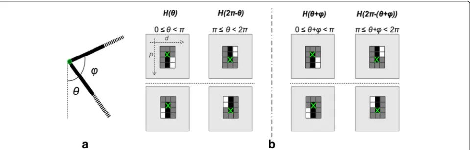
for the planeH(θd)and the same expressions for the cor-responding position of the plane H((θ + ϕ)d), given a certain range ofϕand assumingθ < πand(θ+ϕ) < π.
The value ofηshould be chosen according to the need for detecting approximations of line segment endpoints in curvilinear shapes. Small values ofηprovide additional feature points that are the result of changes of curva-ture on curvilinear boundaries. Nevertheless, these points are less stable than rectilinear corners and segment end-points. Thus, if the stability of detected features along image sequences is essential, greater values ofηmust be chosen.
2.2.1 Reducing the computational complexity
Fig. 6Relation between an image corner and its representation in the 3D Hough space.aImage corner (corner position is represented by agreen circle).bRepresentation of an image corner in the 3D Hough space. Cells associated with the corner are marked with agreen“x”
a cell contains the total number of points belonging to that line. Another important question that should be consid-ered is that, in the discrete parameter space, the relative positions of the cells crossed by a piece of image seg-ment remain the same in several consecutive orientation
planes. Thus, it is not necessary to run the detection pro-cess for every orientation plane, but only for those planes representing a certain increase in angle (φ).
To compute φ, consider the positions (d1,p1) and
(d2,p2)(Eqs. 1 and 2) in a given orientation planeH(θ)of
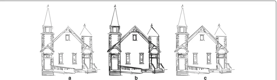
Fig. 8Results of segment detection of the image in Fig. 7a.aDetected segments without considering segment endpoints of neighboring lines.b
Detected segments without non-maximum suppression.cDetected segments using endpoints of neighboring lines and non-maximum suppression
any two image points(x1,y1)and(x2,y2). Assuming that
d1andd2 are the positions indof these two points for an angleθ+φ, the differences indof(x1,y1)and(x2,y2)for
the two angles are related as follows:
(d1−d2)=(d1−d2)cos(φ)+(p1−p2)sin(φ) (10)
Givend1 −d2 ≥ 0 and 0 < φ < π/2, Eq. 10 can be rewritten as:
(d1−d2)≤(d1−d2)+(p1−p2)tan(φ) (11)
Assuming(d1−d2)−(d1−d2)≥01, the last equation
provides an expression of the maximum change of posi-tion in dof the segment defined by (x1,y1) and(x2,y2)
for an increase in angle φ (a similar expression can be obtained for changes inp):
(d1−d2)−(d1−d2)≤(p1−p2)tan(φ) (12)
In order to make this maximum change (Cd) only dependent onφ, the maximum possible value of(p1−p2)
is considered. This value, for pieces of segment formed by ηcells in the Hough representation of corners and end-points, can be set toηp. Thus, Eq. 12 can be rewritten as follows:
Cd =(ηp)tan(φ) (13)
Taking into account the rounding and aliasing effects of the coordinate transformation between image and param-eter spaces, a constant value of 1 pixel forCdis considered, which leads to the following final expression forφ:
φ=arctan 1
ηp (14)
This reduces the number of orientation planes that must be checked for corners and endpoints detection. In addi-tion, since φ andp are inversely related, the increase of computations in each orientation plane caused by a decrease ofpis compensated by a reduction of the
ber of planes where the search must be done. Another important result of this definition forφ is that its value does not change withθ. Thus, reducing the angular res-olution does not increase the computational time of the detection process.
2.2.2 Locating corners and endpoints in the image
Once Hough cells containing corners and endpoints are detected, the next step is to compute their positions in the image. The set of image points belonging to a Hough cell (H(θd,dd,pd)) can be approximated using an image win-dow of sizew×w, withwthe maximum betweendand p, centered on(xc,yc):
xc = dcos(θ)−psin(θ) (15) yc = dsin(θ)+pcos(θ) (16)
with θ,d, and p being the real values associated with θd,dd, and pd. Thus, given a Hough cell (H(θd,dd,pd)) containing a corner or endpoint, locating its image posi-tion can be solved by searching for the pixel within the corresponding image window that maximizes some cor-ner/endpoint criterion. For this purpose, the minimum eigenvalue of the covariance matrix of gradients over the pixel neighborhood is used [29]2. Such a function pro-vides maximum values at corners and endpoints in the point neighborhood.
Figure 7 shows the result of applying this process to a real image. Firstly, using the edge image of Fig. 7b,
Fig. 10Results ofrectangledetection of the image in Fig. 7a
the initial positions of corners/endpoints are obtained by detecting corner/endpoint patterns in the Hough space (Fig. 7c). Then, these positions are adjusted looking for the maximum of the minimum eigenvalue function in the pixel neighborhood (Fig. 7d).
2.3 Detection of segments and polylines
Once corners and endpoints have been extracted, image segments can be detected by checking the strength of any segment formed by a pair of points (Eq. 6). In order to avoid testing segments for every pair of points, detected segment endpoints are placed on the Hough space apply-ing the correspondapply-ing transformation for every orienta-tion value. This provides, for each line representaorienta-tion, a list of points with which segment validation should be done. Assuming that points on that list are ordered by the value of the parameterp, segment detection can be easily solved using Algorithm 3.
Algorithm 3Segment detection 1: forθd=θmin. . .θmaxdo 2: fordd=dmin. . .dmaxdo
3: ifpointList(θd,dd).size() >1then 4: ei←pointList(θd,dd)[0]
5: j←1
6: insertSegment←false
7: maxSS←0
8: whilej<pointList(θd,dd).size()do 9: ej←pointList(θd,dd)[j]
10: newSS←ss(ei,ej)
11: ifnewSS> μsandnewSS>=maxSSthen
12: ef ←ej
13: insertSegment←true
14: maxSS←newSS
15: j←j+1
16: else
17: ifinsertSegmentthen
18: segmentList.add(ei,ef)
19: ei←ef
20: insertSegment←false
21: maxSS←0
22: else
23: ei←ej
24: j←j+1
25: end if
26: end if
27: end while
28: ifinsertSegmentthen
29: segmentList.add(ei,ef) 30: end if
31: end if
In this algorithm,pointList(θd,dd)represents the afore-mentioned list of detected segment endpoints of the line defined by θd and dd. If this list contains at least two points, a segment validation process begins. Given an ini-tial segment endpoint (starting from the first element of the list), this process involves searching for the final end-point of a common line segment (among the subsequent elements of the list) that produces the highest segment strength above a threshold μs. This search stops if the current final endpoint provides a lowerstrengththan the previous one. In such a case, the previous validated seg-ment is stored and the process is restarted taking the last valid final endpoint as the initial endpoint of a new segment.
The rounding step of the coordinate transformation between image and Hough spaces could make an almost vertical segment divide into two pieces. To deal with this problem, if an image corner or endpoint falls near a cell
of the neighboring line, it is included in the list of points of that line. This mostly solves the segment breakdown problem, although it may increase the number of false positives. Nevertheless, they can be discarded applying a subsequent non-maximum suppression step to the seg-ments with a common endpoint. Thus, taking the angle defined by two segments with a common endpoint as a proximity measure, if two segments are considered near enough, the one with the smallest strength is removed from the set of detected segments.
Figure 8 shows the result of detecting the segments of image in Fig. 7a using the corners and endpoints of Fig. 7d. Figure 8a shows the result of segment detection with-out considering segment endpoints of neighboring lines. Figure 8b shows the result of using endpoints close to each line without applying the non-maximum suppression pro-cess. Finally, Fig. 8c depicts detected segments using extra endpoints with non-maximum suppression.
Since segments are confirmed from their endpoints, they are implicitly interconnected forming polylines. These polylines can be extracted from the graph repre-sentation that is obtained taking endpoints as vertices and segments as edges connecting vertices. Thus, each disconnected subgraph resulting from this representation corresponds to a polyline in the image. In the ideal case, when each node has one or two edges, this is the only valid interpretation of the graphs. However, if there exist vertices with more than two connections, each polyline can be decomposed into simple pieces. In such cases, a graph partitioning technique [30] can be applied in order to obtain a more realistic polyline representation.
2.4 Computational complexity of the corner and segment detection method
The analysis of the computational complexity of the pro-posed corner and segment detection method can be
studied by considering its five different phases: (a) first stage of the voting process (line voting); (b) second stage of the voting process (accumulation); (c) corner/endpoint detection; (d) corner/endpoint mapping between image and Hough spaces; and (e) segment detection. Assuming the Hough space is formed bylorientation planes of size m×mand takingnas the number of edge points, the two stages of the voting process can be performed with com-putational costsO(mn)andO(lm2), respectively. Using a single voting process would entail a computational cost of O(lmn) instead. It must be noted that generally n is much bigger thanm, so in practice, the two-stage voting scheme is much less time-consuming. Corner detection is solved with a computational cost ofO(lrm2), with lr being the number of orientation planes usingφ (Eq. 14) as angle resolution. lr is significantly smaller than any of the dimensions of the Hough space, so this computa-tional cost can be considered sub-cubic. Takingpas the
number of detected corners/endpoints, the mapping of these points from the image space to the Hough space, as a previous step to segment detection, is achieved with cost O(lp). This is also the computational cost of seg-ment detection, since each plane will containppoints and each point can at most confirm two segments in the same orientation plane.
Despite all the included optimizations, the proposed method presents a clearly higher computational cost than many existing approaches for independent detection of corners and line segments. Nevertheless, all its phases iteratively carry out the same processing over indepen-dent elements of both image and Hough spaces, which makes them inherently parallelizable. Taking advantage of this, we have developed a parallel implementation of the proposed corner and segment detector on a GPU. This implementation attempts to approximate the computa-tional cost of each phase to linear time in relation to the
image size. Regarding the sequential version, speedups above 400×in some of the phases and about 35×in the whole method, including data exchanges between CPU and GPU, have been obtained3. Although this implemen-tation significantly outperforms its sequential counter-part, we are working on new optimizations to improve the speedup dealing with GPU programming issues such as coalesce memory accesses and optimal occupancy.
2.5 Detection of other image features
As explained above, the segment detection process pro-vides not only a set of segments but also a set of polygo-nal chains. These polygopolygo-nal chains have arbitrary shapes since they are the result of the implicit connection of the detected segments. Nevertheless, the proposed Hough space can also be used for the detection of predefined polygonal shapes. One of the simplest cases is the detec-tion of rectangles [31, 32].
Since a rectangle is composed of four segments, the 3D Hough space makes it possible to compute the total number of points included in the contour of the rectan-gle. Thus, considering a rectangle expressed by its four verticesV1 = (x1,y1),V2 = (x2,y2),V3 = (x3,y3), and
V4 = (x4,y4) (see Fig. 9), the number of points of its
contour, denoted asHr, can be computed as:
Hr =H1↔2+H2↔3+H3↔4+H4↔1 (17)
where each Hi↔j denotes the number of points of the segment defined byViandVj(Eq. 5).
Figure 9 shows an example of rectangle representation in the discrete parameter space. Each pair of parallel seg-ments of the rectangle is represented in the corresponding orientation plane of the Hough space:H(αd)for one pair of segments andH((α+π/2)d) for the other one, with αd and(α+ π/2)d being the discrete values associated toα (rectangle orientation) and(α+π/2), respectively.
For each orientation plane, there is a representation of how many points contribute to each cell (dd,pd), i.e., how many points belong to every segment of the corre-sponding orientation. A high histogram contribution is represented in the figure with a dark gray level, while a low contribution is depicted with an almost white color. As it can be observed, the highest contributions are found in parallel segments with displacements of wd and hd, which are the discrete values associated to the rectangle dimensions.
Taking this rectangle representation into account and considering continuous values of each parameter for sim-plification, eachHi↔jof expression 17 can be rewritten as follows:
H1↔2= |H(α,d1↔2,d4↔1)−H(α,d1↔2,d2↔3)| (18)
H2↔3= |H(α+π/2,d2↔3,−d1↔2)
−H(α+π/2,d2↔3,−d3↔4)| (19)
H3↔4= |H(α,d3↔4,d2↔3)−H(α,d3↔4,d4↔1)| (20)
H4↔1= |H(α+π/2,d4↔1,−d3↔4)
−H(α+π/2,d4↔1,−d1↔2)| (21)
with di↔j being the parameter d of the straight line defined by the pointsViandVj, which are related with the rectangle dimensions as follows
w=d3↔4−d1↔2 (22)
h=d2↔3−d4↔1 (23)
According to these expressions, rectangle detection can be solved by searching for those combinations of (α,d1↔2,d2↔3,d3↔4,d4↔1)for whichHr/(2∗w+2∗h) > τr, given a certain value ofτr near to 1. To improve the efficiency of this process, instead of checking each combi-nation of these parameters, previously detected segment endpoints can be used to preselect an initial subset of
Table 1Number of detected corners/endpoints (NEpd) for the ten test images
NEpd
FAST Harris HT3D
1 273 330 375
2 318 401 477
3 1084 1165 1369
4 1306 1315 1753
5 833 910 1336
6 1400 1662 1984
7 1139 1264 1341
8 1395 1561 1866
9 799 846 1108
10 1615 1714 1950
combinations. Thus, a similar procedure to the one shown in Algorithm 3 can be applied forθ < π/2 to find the first segment of a potential rectangle, which provides values for α,d1↔2,d2↔3andd4↔1. Then, using the list of points of
the Hough line corresponding tol(d2↔3,α+π/2),
possi-ble values ford3↔4are obtained, completing the quintuple
defining a rectangle.
Figure 10 shows the result of applying the above pro-cess to the image in Fig. 7a. During the detection propro-cess, the segment endpoints of Fig. 7d are used for restrict-ing the parameters of potential rectangles as previously described.
3 Results and discussion
To evaluate the performance of the proposed detec-tion methods, they have been applied to a set of real images with ground truth. This section shows the results,
comparing them with the ones obtained using other approaches.
A critical point when using an HT-based approach is to decide the resolutions of the parameter space. Finer quantizations do not always provide better results. Indeed, noise sensitivity grows for higher precision with regard to d[33]. Zhang [34] proposes determiningdby con-sidering the digitization of the spatial domain and then computesθusing the following relation:
nd= lθ
2d (24)
withndwithin the interval [0.5, 2] andlthe length of the longest line segment.
Fixing a value for d (and also for p) depends not only on the need for a detailed result but mainly on the nature of the image. Thus, for a noisy image, the detection method will perform better using a value ofd that is not too small. In addition, if the image complexity is not too high, understanding complexity in terms of the num-ber and distribution of edge point chains, a low value of dwill provide a similar result to a higher one. For the test images used to evaluate our proposal, a value of 2 for d and p has been chosen. However, it must be pointed out that, for some of them, higher resolutions pro-duce a comparable detection rate.θhas been fixed using expression 24 withnd=1 andl=400.
Results for corner and segment detection have been obtained using the YorkUrbanDB dataset [35]. This dataset contains 102 marked images of urban environ-ments. Each image is labeled to identify the subset of line segments that satisfy theManhattan assumption[36]. Both quantitative and qualitative evaluations have been carried out for the whole set of images, comparing our corner and segment detector (HT3D) with two corner
Table 2Comparison of detected corners/endpoints with the ground truth for the ten test images
NEpc
FAST Harris HT3D
dEp 4 3 2 4 3 2 4 3 2
NEPg
1 78 35 33 25 45 40 32 53 47 33
2 222 118 96 70 127 115 93 143 128 99
3 170 81 71 59 93 90 73 125 120 94
4 1104 551 471 359 552 497 406 710 631 508
5 538 230 197 133 238 208 160 347 284 213
6 790 408 364 281 452 410 359 524 488 406
7 644 265 227 171 293 262 234 352 323 271
8 577 336 289 201 369 333 234 394 354 297
9 248 106 94 67 112 103 90 146 137 117
10 346 190 170 138 215 197 175 246 220 189
Fig. 16Ratio betweenNEpc(number of correct matchings between ground truth and detected points) andNEpd(total number of detected points)
for the whole dataset consideringdEp=3 (distance between ground truth and detected points). A low value of this ratio for one detector in
relation to other methods is indicative of a high number of false alarms. As it can be observed in this figure, the ratio remains almost constant in the three methods for most of the test images, which denotes similar rates of false alarms in the three detectors
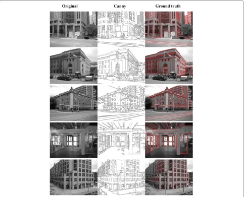
detectors and two segment detectors. A quantitative com-parison of the different approaches using the 102 images composing the dataset is shown here. Complete results for a subset of ten images are also included. This subset corre-sponds to the ten scenes of Figs. 11 and 12. For each scene, these figures show the original image, the Canny image, used as input in our approach, and the ground truth. Every image has been smoothed using a 5×5 Gaussian filter with a standard deviation of 1 before being applied to each method, except for one of the segment detectors (LSD), since it includes its own smoothing step.
For corner and endpoint detection, our method has been compared with Harris [37] and FAST [38].
Parameters of these methods have been experimentally chosen trying to favor the detection results as much as possible according to the relation between true and false corners. Specifically, for the Harris method, a neighbor-hood size of 5 pixels and a sensitivity factor of 0.04 have been used. Likewise, the intensity comparison threshold of FAST has been set to 15. In the proposed method, a length of 4 cells has been taken for the pieces of seg-ments defining corners and endpoints in the Hough space (parameterη). Also, the angle range to confirm corners has been set to [75◦, 105◦].
Figures 13 and 14 show the corner/endpoint detection results for the two sets of images in Figs. 11 and 12
Fig. 17Ratio betweenNEpc(number of correct matchings between ground truth and detected points) andNEpd(total number of detected points)
for the whole dataset consideringdEp=2 (distance between ground truth and detected points). No significant variations of this ratio can be
Fig. 18Ratio betweenNEpc(number of correct matchings between ground truth and detected points) andNEpg(number of ground truth points)
for the whole dataset consideringdEp=3 (distance between ground truth and detected points). This ratio quantifies the hit rates of the three corner
detection methods. In general, clearly higher hit rates can be observed when using the proposed method in the large majority of the test images
using FAST, Harris, and the proposed method. Figure 15 shows some representative regions of these images where the differences among the detection results of the com-pared approaches can be clearly appreciated. As it can be observed, the three methods perform well in the detec-tion of corners resulting from the intersecdetec-tion of straight perpendicular edges. However, in most cases, the pro-posed method provides additional corner points. Some of them correspond to corners with non-right angles, mainly obtuse-angle corners, and to corners with low intensity
in one of its edges (see the first three rows of images in Fig. 15). In addition, as it was expected, only our method detects non-intersection segment endpoints (see the last two rows of Fig. 15). They can be mostly found in the intersections between image lines and image limits. All these additional distinctive points are essential for line segment detection.
In order to quantitatively evaluate the three methods, each group of detected points has been compared with the segment endpoints of the ground truth data. Three
Fig. 19Ratio betweenNEpc(number of correct matchings between ground truth and detected points) andNEpg(number of ground truth points)
for the whole dataset consideringdEp=2 (distance between ground truth and detected points). The hit rates of the proposed method remain
higher than the hit rates of the other two methods when reducingdEp. No significant differences in the accuracy of the three methods can be
measures were considered in this comparison: number of detected corners/endpoints (NEpd), number of points of the ground truth data (NEpg), and number of cor-rect matchings between ground truth and detected points (NEpc). To compute NEpc, different values of the max-imum euclidean distance (dEp) between detected and ground truth points were considered. Tables 1 and 2 show the results obtained for the ten test images. Table 1 contains the total number of detected corners/endpoints using each method. Table 2 shows the number of ground truth points of each image and the number of correct matchings of the different detectors taking values of 4, 3, and 2 fordEp. Results show greater values ofNEpd in HT3D than in FAST and Harris, although NEpc grows linearly. This behavior can also be observed in the entire dataset from the results depicted in Figs. 16 and 17. These figures show the ratio betweenNEpcandNEpdfor each image of the dataset considering values fordEpof 3 and
2, respectively. Since the ground truth only includes a subset of potential line segments, false alarm rates can-not be directly measured. Nevertheless, the ratio between the number of correct matchings and the total number of detected features constitutes a false alarm indicator in the comparison among different methods. Thus, if a method presents a clearly low value of this ratio in relation to other approaches, it can be stated that the number of false detec-tions of that method is significantly higher. For the present comparison among the corner/endpoint detectors, as it can be seen in Figs. 16 and 17, the ratio remains almost constant in the three methods for all the tests, which denotes similar rates of false detections in all of them. In relation to the hit rate of each approach, which has been measured as the ratio between the number of correct matchings and the number of ground truth points, Figs. 18 and 19 show higher values for HT3D than for the other two methods, regardless of the value ofdEp. Thus, on the
basis of this ratio, HT3D performs better than FAST in almost 100% of the images and better than Harris in about 95% of the tests. Since the difference among the hit rates of the three detectors does not significantly vary when reducingdEp, the accuracy provided by all the methods can be considered comparable.
Regarding segment detection, our method has been compared with two segment detectors: PPHT [19] (see Section 1 for a brief description) and LSD [39], a non-Hough-based line segment detector, which works without parameter tuning. In PPHT, the parameter space has been discretized using values of 1 andπ/180 for distance and angle resolutions. Also, a minimum number of line votes of 20 and a value of 5 for the minimum segment length and the maximum gap of points of the same line have been used. In our method, segments have been detected con-sidering a minimum segment strengthof 0.8. Results of both Hough-based methods have been obtained from the same edge images.
The detected segments using the three methods for the ten test images are displayed in Figs. 20 and 21. Some zoomed representative regions of these images are shown in Fig. 22. The three segment detectors have also been quantitatively evaluated considering, firstly, the number of detected segments (NSd) and the percentage of con-nected segments (CS). In images of real environments, segments do not usually appear as isolated entities, but as part of more complex features that allow object con-tours to be described. This is especially true in man-made environments, where, for instance, windows, doors, and walls are composed of sets of segments which are con-nected forming polylines. In this regard, we believe that the ability of a segment detector to obtain not individ-ual segments but chains of segments makes the detec-tion results more reliable. Table 3 shows a quantizadetec-tion of the segment-connectivity ability of the three meth-ods through the measurementCS. As it can be observed, PPHT, with the chosen parametrization, does not provide
Fig. 22Zoomed representative regions of the images in Figs. 20 and 21. In this figure, the differences in the line segment detection results of the three methods can be clearly appreciated
any connections among detected segments for any of the test images. Detected segments from LSD do present some degree of connectivity, but the connectivity rate is much lower than the one obtained by HT3D, which pro-vides results in greater accordance with the kind of scenes in the image set.
Results of the three segment detector have also been compared with the ground truth data, using the Hausdorff distance [40] to determine the correct matchings. Given
two segmentssi = (ei1,ei2)andsj = (ej1,ej2), the
Haus-dorff distance betweensi andsj, denoted as hd(si,sj), is defined as follows:
hd(si,sj)=min(max(|ei1−ej1|,|ei2−ej2|),
max(|ei1−ej2|,|ei2−ej1|))
(25)
Table 3Number of detected segments (NSd) and percentage of connected segments (CS) for the ten test images
PPHT LSD HT3D
NSd CS(%) NSd CS(%) NSd CS(%)
1 352 0 329 21 263 67
2 434 0 515 13 335 74
3 1847 0 751 17 912 69
4 2376 0 1274 15 1213 77
5 1655 0 838 13 907 63
6 2768 0 1034 20 1321 62
7 1079 0 1058 14 924 76
8 2622 0 1112 14 1269 62
9 1295 0 839 15 738 71
10 2194 0 1301 28 1355 77
The percentage of connected segments is indicative of the ability of a segment detector to provide chains of segments corresponding to the polygonal image contours. According to this measure, the proposed method (HT3D) produces clearly better results than the other two approaches
greater than a maximum distance dS. Using this crite-rion, Table 4 shows the number of correct matchings (NSc) of the three methods from the total number of ground truth segments (NSg) considering values of 4, 3, and 2 for dS. From the results obtained, it can be seen that PPHT detects a lower number of correct matchings than the other two approaches, even though the total number of detected segments is considerably greater in many cases. LSD clearly improves on the results of PPHT, but the hit rates are generally lower than those provided by HT3D. The difference in performance between HT3D and the other two segment detectors becomes more evident as
Table 4Comparison of detected segments with the ground truth for the ten test images
NSc
PPHT LSD HT3D
dS 4 3 2 4 3 2 4 3 2
NSg
1 42 5 4 3 18 12 4 24 21 9
2 120 21 17 11 64 47 17 75 61 45
3 111 23 13 5 59 43 19 59 47 32
4 628 92 56 20 272 174 61 291 236 124
5 306 58 34 17 120 65 23 124 82 37
6 434 57 34 12 174 112 32 194 158 89
7 373 54 27 9 154 101 46 155 121 73
8 350 70 44 13 159 105 42 155 113 61
9 139 14 11 5 45 30 18 60 50 29
10 209 70 54 36 136 112 45 159 145 92
The number of correct matchings of each method (NSc) is shown considering different values of the distance between ground truth and detected segments (dS). The total number of ground truth segments (NSg) is shown in the first column
dS decreases. This can be observed, not only in the ten test images but also in the whole dataset, through the results depicted in Figs. 23, 24, 25 and 26. These figures show the ratiosNSc/NSdandNSc/NSg4for each image of the dataset considering values of 3 and 2 fordS. Regard-ing the ratio between the number of correct matchRegard-ings and the total number of detected segments (NSc/NSd), HT3D gives much greater values than PPHT in almost 100% of the tests for the different values ofdS. The main reason is that PPHT detects a high rate of false posi-tives, which considerably diminishes this ratio. They can be reduced by increasing the minimum number of line votes, but at the expense of proportionally reducing the number of correct matchings. In HT3D, false positives are avoided by requiring that Hough cells in contigu-ous positions to the ones defining a segment do not also define full segments on both sides. This solves to a great extent the problem of detecting false segments, although this means that parallel segments must be situated some distance away from each other in order to be correctly detected.
In relation to the comparison between HT3D and LSD, although the differences are less notable than in the com-parison with PPHT, better results are obtained in most cases when using HT3D. Differences between the results of both methods become more obvious fordS = 2. The principal cause is that segments detected by LSD repeat-edly break off before reaching their actual endpoints. In addition, when segments are crossed by other segments, they break into shorter segments, which affects not only the number of correct segments but also the total number of detected segments. Both problems also occur in PPHT (see Fig. 22).
Fig. 23Ratio betweenNSc(number of detected segments matching the ground truth data) andNSd(total number of detected segments) for the
whole dataset consideringdS=3 (distance between ground truth and detected line segments). Higher values of this ratio can be observed in most
of the test images for the proposed method when comparing with the other two approaches. This indicates a better performance of HT3D in relation to LSD and PPHT. In addition, the low values associated to PPHT are indicative of a high number of false detections
some structures, the proposed method correctly detects most of the rectangular contours. There are some false detections caused by two different factors. False positives corresponding to small areas are due to the fact that these kinds of regions are less affected by edge gaps than bigger ones and so they should be confirmed with higher values ofτr. In this sense, instead of using a constant threshold, a variable threshold obtained as a function of the region size should be applied to improve the results. The other group of false detections corresponds to areas close to actual rectangular regions that share several corners with them. For better performance, those rectangles sharing more than one corner and presenting a similar orientation must be separately analyzed to determine which of them
are finally considered. Both improvements, however, are beyond the scope of this paper since they are specific to rectangle detection.
4 Conclusions
This paper presents an extension of the Hough Transform, called HT3D, for the combined detection of corners, seg-ments, and polylines. This new variant of HT uses a 3D parameter space that facilitates the detection of segments instead of lines. It has been shown how this representa-tion also encloses canonical configurarepresenta-tions of corners and non-intersection endpoints, making it a powerful tool, not only for the detection of line segments but also for the extraction of such kinds of points.
Fig. 24Ratio betweenNSc(number of detected segments matching the ground truth data) andNSd(total number of detected segments) for the
whole dataset consideringdS=2 (distance between ground truth and detected line segments). The differences among the three methods when
Fig. 25Ratio betweenNSc(number of detected segments matching the ground truth data) andNSg(total number of segments of the ground truth
data) for the whole dataset consideringdS=3 (distance between ground truth and detected line segments). This ratio measures the hit rates of the
three methods for every test image. In general, it is possible to observe a greater correspondence of the results provided by the proposed method with the ground truth data
One of the main novelties of our proposal is that line segments are not directly searched for in the image. Instead, they are verified from their endpoints using a segment measure obtained from the segment represen-tation provided by the Hough space. This makes line segment detection robust to line gaps, edge deviations, and crossing lines. In addition, this segment detection strategy improves the accuracy of the results in relation to other approaches. Thus, methods based on the analysis of edge or gradient information in the image space miss the
actual boundaries of line segments, since gradient at those points presents a high uncertainty [28]. Instead of building chains of aligned edge pixels, the presented approach con-firms the existence of line segments between couples of previously detected endpoints. Experiments have shown how thisinversestrategy provides more accurate results than the segment generation approach. The main draw-back of using a segment measure is that it could produce high responses for non-real line segments in noisy or complex images. False positives are mainly false segments
Fig. 26Ratio betweenNSc(number of detected segments matching the ground truth data) andNSg(total number of segments of the ground truth
data) for the whole dataset consideringdS=2 (distance between ground truth and detected line segments). Differences in the hit rates between
the proposed method and the other two approaches for segment detection become more obvious when reducingdS. This denotes the greater
Fig. 27Set of images used for testing the proposed rectangle detection method
crossing several real segments. Thus, false detections can be controlled by requiring that the Hough cells situated in contiguous positions to the pair of cells defining a line segment do not produce high values for the segment mea-sure. Depending on the resolution of the Hough space, this additional criterion might discard true positive detections corresponding to close parallel line segments. Neverthe-less, it significantly reduces the number of false positives, producing reliable results.
Regarding corner detection, our proposal provides an alternative to intensity-based detectors. These methods present some limitations in the detection of corners of obtuse angles, since in the local environment of those points significant intensity changes are only perceived in one direction [42]. In our approach, corners are con-sidered as image points intersecting two line segments at a given angle range. This corner definition is con-sistent with certain cell patterns in the Hough space.
Fig. 29Detected rectangles in the Fig. 27 images
Thus, applying a pattern matching process, corners are detected in the Hough space and then located in the image space. If a corner is identified in the Hough space, it is accepted as a valid detection and the intensity image is only used to find the most likely pixel position associ-ated to the corresponding corner position in the Hough space. This coarse-to-fine method avoids applying any threshold related to changes of intensity in the corner local environment, which allows the identification of cor-ner points that other methods miss. The same proposed strategy for corner detection is also used for detecting other kinds of distinctive points corresponding to seg-ment endpoints that do not intersect other line segseg-ments. This set of points, called non-intersection endpoints, is key for obtaining reliable results in the detection of seg-ments, since segment endpoints do not always correspond to corners. The experimental evaluation presented in this paper shows good detection rates of both types of points when comparing with the ground truth. Thus, our pro-posal matches up to 20% more ground truth points than the compared methods.
Besides the accuracy benefits, the combined detection of corners and line segments produces the direct identi-fication of polygonal structures in the image, which has additional applications. Moreover, we have shown how the segment measure can be extended to detect predefined polygonal shapes, which are important image features in a variety of problems, such as those related to the identification of man-made structures in aerial images.
The whole detection method entails five processing stages on a 3D memory structure, so it presents a
higher computational complexity than methods devoted to the detection of individual features. Nevertheless, all the stages present a characteristic structure that makes them inherently parallelizable. In this regard, some initial results of a parallel implementation of the method have been obtained, showing a significant time reduction. We are working on this parallel implementation and devel-oping new optimizations to reduce execution times even further.
Endnotes
1Otherwise, the same reasoning can be done using the
expressions ofd1andd2from(d1,p1)and(d2,p2)instead
of Eq. 10.
2It must be noted that this function is only computed
for those pixels detected as potential corners/endpoints in the Hough space and not for the whole image.
3These results have been obtained on images of size
640×480 with around 15% edge points using an Intel i7 2.67 GHz processor for the sequential version and a NVIDIA GTX 1060 GPU for the parallel implementation.
4Both ratios remain moderate in all the methods for
Acknowledgements
This work has partly been supported by grants TIN2015-65686-C5-5-R and PHBP14/00083, from the Spanish Government.
Authors’ contributions
PBB wrote the main part of this manuscript. LJM modified the content of the manuscript. PB participated in the discussion. All authors read and approved the final manuscript.
Competing interests
The authors declare that they have no competing interests.
Publisher’s Note
Springer Nature remains neutral with regard to jurisdictional claims in published maps and institutional affiliations.
Received: 2 August 2016 Accepted: 12 April 2017
References
1. A De la Escalera, JM Armingol, Automatic chessboard detection for intrinsic and extrinsic camera parameter calibration. Sensors.10(3), 2027–2044 (2010)
2. L Forlenza, P Carton, D Accardo, G Fasano, A Moccia, Real time corner detection for miniaturized electro-optical sensors onboard small unmanned aerial systems. Sensors.12(1), 863–877 (2012)
3. R Chandratre, VA Chakkarwar, Article: Image stitching using harris and ransac. Int. J. Comput. Appl.89(15), 14–19 (2014)
4. A Dick, P Torr, R Cipolla, inProceedings of the British Machine Vision Conference. Automatic 3d modelling of architecture (BMVA Press, UK, 2000), pp. 39–13910
5. P Kahn, LJ Kitchen, EM Riseman, A fast line finder for vision-guided robot navigation. IEEE Trans. Pattern Anal. Mach. Intell.12(11), 1098–1102 (1990)
6. CX Ji, ZP Zhang, Stereo match based on linear feature. ICPR.88, 875–878 (1988)
7. P Fränti, E Ageenko, H Kälviäinen, S Kukkonen, inProc. Fourth Joint Conference on Information Sciences JCIS’98. Compression of Line Drawing Images Using Hough Transform for Exploiting Global Dependencies (Association for Intelligent Machinery, Research Triangle Park, 1998), pp. 433–436
8. H Moon, R Chellappa, A Rosenfeld, Performance analysis of a simple vehicle detection algorithm. Image Vis. Comput.20(1), 1–13 (2002) 9. S Noronha, R Nevatia, Detection and modeling of buildings from multiple
aerial images. IEEE Trans. Pattern Anal. Mach. Intell.23(5), 501–518 (2001) 10. Y Zhu, B Carragher, F Mouche, CS Potter, Automatic particle detection
through efficient Hough transforms. IEEE Trans. Med. Imaging.22(9), 1053–1062 (2003)
11. PVC Hough, Method and means for recognizing complex patterns. Google Patents. Patent 3, US 069,654 (1962). http://www.google.com/ patents/US3069654. Accessed Apr 2017
12. P Mukhopadhyay, BB Chaudhuri, A survey of Hough Transform. Pattern Recognit.48(3), 993–1010 (2014)
13. RO Duda, PE Hart, Use of the Hough transformation to detect lines and curves in pictures. Commun. ACM.15(1), 11–15 (1972)
14. Y Ching, Detecting line segments in an image—a new implementation for Hough Transform. Pattern Recognit. Lett.22(3/4), 421–429 (2001) 15. H Duan, X Liu, H Liu, inPervasive Computing and Applications, 2007. ICPCA
2007. 2nd International Conference On. A nonuniform quantization of hough space for the detection of straight line segments (IEEE, Birmingham, 2007), pp. 149–153
16. LAF Fernandes, MM Oliveira, Real-time line detection through an improved Hough transform voting scheme. Pattern Recognit.41(1), 299–314 (2008)
17. J Song, MR Lyu, A hough transform based line recognition method utilizing both parameter space and image space. Pattern Recognit.38(4), 539–552 (2005)
18. G Gerig, inProc. of First International Conference on Computer Vision. Linking image-space and accumulator-space: a new approach for object recognition (Computer Society Press of the IEEE, London, 1987), pp. 112–117
19. J Matas, C Galambos, J Kittler, Robust detection of lines using the progressive probabilistic hough transform. Comput. Vis. Image Underst. 78(1), 119–137 (2000)
20. TT Nguyen, XD Pham, J Jeon, inProc. IEEE Int. Conf. Industrial Technology. An improvement of the standard hough transform to detect line segments (IEEE, Chengdu, 2008), pp. 1–6
21. J Cha, RH Cofer, SP Kozaitis, Extended Hough transform for linear feature detection. Pattern Recognit.39(6), 1034–1043 (2006)
22. S Du, BJ van Wyk, C Tu, X Zhang, An improved Hough transform neighborhood map for straight line segments. Trans. Img. Proc.19(3), 573–585 (2010)
23. S Du, C Tu, BJ van Wyk, EO Ochola, Z Chen, Measuring straight line segments using ht butterflies. PLoS ONE.7(3), 1–13 (2012)
24. Z Xu, B-S Shin, inImage and Video Technology. Lecture Notes in Computer Science. Line segment detection with Hough transform based on minimum entropy, vol. 8333 (Springer, Berlin Heidelberg, 2014), pp. 254–264
25. ER Davies, Application of the generalised hough transform to corner detection. IEE Proc. E (Comput. Digit. Tech.)135, 49–545 (1988) 26. DH Ballard,Readings in computer vision: issues, problems, principles, and
paradigms, Chap. Generalizing the Hough Transform to Detect Arbitrary Shapes. (Morgan Kaufmann Publisher Inc., San Francisco, 1987), pp. 714–725
27. WA Barrett, KD Petersen, inComputer Vision and Pattern Recognition, 2001. CVPR 2001. Proceedings of the 2001 IEEE Computer Society Conference On, vol. 2. Houghing the hough: peak collection for detection of corners, junctions and line intersections (IEEE, Kauai, 2001), pp. 302–3092 28. F Shen, H Wang, Corner detection based on modified hough transform.
Pattern Recognit. Lett.23(8), 1039–1049 (2002)
29. J Shi, C Tomasi, in1994 IEEE Conference on Computer Vision and Pattern Recognition (CVPR’94). Good features to track (Cornell University, Ithaca, 1994), pp. 593–600
30. Buluç, H Meyerhenke, I Safro, P Sanders, C Schulz, Recent advances in graph partitioning. CoRR.abs/1311.3144, 1–37 (2013)
31. MA Gutierrez, P Bachiller, L Manso, P Bustos, Nú, P,ñez, inProceedings of the 5thEuropean Conference on Mobile Robots, ECMR 2011, September 7-9,
2011, Örebro, Sweden. An incremental hybrid approach to indoor modeling (Learning Systems Lab, AASS, Örebro University, Örebro, 2011), pp. 219–226
32. P Bachiller, P Bustos, LJ Manso, inAdvances in Stereo Vision, ed. by JRA Torreao. Attentional behaviors for environment modeling by a mobile robot (InTech, Croatia, 2011), pp. 17–40
33. V Shapiro, Accuracy of the straight line hough transform: The non-voting approach. Comp. Vision Image Underst.103(1), 1–21 (2006)
34. M Zhang, inIn Proc. of IEEE (ICPR’96). On the discretization of parameter domain in Hough transformation (IEEE Computer Society, Los Alamitos, 1996), pp. 527–531
35. P Denis, JH Elder, FJ Estrada, inECCV (2). Lecture Notes in Computer Science, ed. by DA Forsyth, PHS Torr, and A Zisserman. Efficient edge-based methods for estimating manhattan frames in urban imagery, vol. 5303 (Springer, Berlin Heidelberg, 2008), pp. 197–210
36. JM Coughlan, AL Yuille, Manhattan world: orientation and outlier detection by bayesian inference. Neural Comput.15, 1063–1088 (2003) 37. C Harris, M Stephens, inProc. of Fourth Alvey Vision Conference. A
combined corner and edge detector (Organising Committee AVC 88, Manchester, 1988), pp. 147–151
38. E Rosten, T Drummond, inProceedings of the 9th European Conference on Computer Vision - Volume Part I. ECCV’06. Machine learning for high-speed corner detection (Springer-Verlag, Berlin, 2006), pp. 430–443
39. R Grompone von Gioi, J Jakubowicz, J Morel, G Randall, Lsd: a line segment detector. Image Processing On Line.2, 35–55 (2012) 40. J Henrikson, Completeness and total boundedness of the Hausdorff
metric. MIT Undergrad. J. Math.1, 69–80 (1999)
41. J Yuan, SS Gleason, AM Cheriyadat, Systematic benchmarking of aerial image segmentation. IEEE Geosci. Remote Sensing Lett.10(6), 1527–1531 (2013)