RESEARCHARTICLE
Discovery of topological constraints
on spatial object classes using a
refined topological model
Ivan Majic, Elham Naghizade, Stephan Winter, and Martin
Tomko
Department of Infrastructure Engineering, The University of Melbourne, Australia
Received: August 16, 2018; returned: September 25, 2018; revised: November 6, 2018; accepted: February 7, 2019.
Abstract: In a typical data collection process, a surveyed spatial object is annotated upon creation, and is classified based on its attributes. This annotation can also be guided by tex-tual definitions of objects. However, interpretations of such definitions may differ among people, and thus result in subjective and inconsistent classification of objects. This problem becomes even more pronounced if the cultural and linguistic differences are considered. As a solution, this paper investigates the role of topology as the defining characteristic of a class of spatial objects. We propose a data mining approach based on frequent itemset mining to learn patterns in topological relations between objects of a given class and other spatial objects. In order to capture topological relations between more than two (linear) objects, this paper further proposes a refinement of the 9-intersection model for topological relations of line geometries. The discovered topological relations form topological con-straints of an object class that can be used for spatial object classification. A case study has been carried out on bridges in the OpenStreetMap dataset for the state of Victoria, Australia. The results show that the proposed approach can successfully learn topological constraints for the class bridge, and that the proposed refined topological model for line geometries outperforms the 9-intersection model in this task.
1
Introduction
Responsive maintenance of spatial data and its quality is becoming difficult due to the increase of the volume of collected data and its heterogeneity. In the traditional data collec-tion processes, when a spatial object is created it is annotated with attributes, where at least the class of the object it belongs to is captured (e.g., a spatial object annotated as a bridge be-longs to the bridge class). To help with this process of annotation, textual definitions of the class semantics are supplied in taxonomies (or object catalogues) and often standardized for interoperability. The association of a surveyed or manually vectorized spatial object with an object class is performed by a human operator, interpreting the definition and de-ciding which class the object belongs to. This may happen during data collection (e.g., a surveyor annotating the measured geometries) or in a separate, consecutive process.
Consider the definition of abridgefrom the Merriam-Webster dictionary: “a structure carrying a pathway or roadway over a depression or obstacle (such as a river).”Such a classifica-tion is problematic because it depends on human judgment. (Is what this bridge carries a pathwayor aroadway? Could arailwayalso be carried by abridge?) Uncertainty in the inter-pretation of a definition leads to inconsistent or even erroneous object classifications across the dataset, especially if performed by different operators [3]. This is becoming a salient problem in the context of global datasets where cultural and linguistic differences may im-pact the definition interpretations [30]. Furthermore, volunteered geographic datasets [20], such as OpenStreetMap (OSM) often do not prescribe strict object classifications and often impose only vague and fluid rules. For example, the OSM wiki page for the attribute key bridgedescribes a bridge as “an artificial construction that spans features such as roads, railways, waterways or valleys and carries a road, railway or other feature.” It also lays out guidelines on how to map and tag a bridge. However, none of these guidelines are enforced in OSM, so contributors can map and tag bridges however they see fit. Hence, the question arises: how can the classification of spatial objects be improved and the quality of classification assured efficiently in a way that does not require ground truth?
A number of classes of spatial objects are defined not only by their attributes, but also through their functional properties, stemming from their spatial configuration with respect to other objects. Arguably, a defining feature of abridgeis that itcarriesaway oversome obstacle, rather than the distinction between the carried structure being a pathway, roadway, or railroad. Thus, following the notion that topology matters and metric refines [18], this paper investigates the role of topology as the defining (although possibly not the sole) characteristic defining the class of certain spatial objects.
Based on the observation that topology defines the function of many spatial objects, we hypothesize that patterns in topological relations between spatial objects in large spatial datasets can be analyzed to classify spatial objects. Thus, the detailed questions addressed in this paper are:
• How can the topological relations between spatial objects be effectively analysed to find patterns?
• How can the patterns in topological relations be used to define classes of spatial ob-jects?
relations between these objects and other spatial objects that are not disjoint from them. This paper shows that for some classes of spatial objects, topological relations are charac-teristic and defining. The aim of this research is to discover topological relations that form topological constraints of an object class and can be used (possibly with other attributes and geometrical properties) either to correct inconsistencies in spatial databases, or to infer the class of newly imported spatial objects.
Furthermore, this paper also proposes a refinement of the 9-intersection model of topo-logical relations of line geometries [17]. The existing model is characterizing binary re-lations and cannot describe scenarios where more than two objects are involved. This is particularly important in networks, where there may be the need to show that a certain segment is connected to the rest of the network on both sides. Thus, the refinement pro-posed here examines whether the core line object is connected to its surrounding objects on both or only one of its ends (i.e., start and end point).
This paper makes the following contributions:
• It shows that topology strongly contributes to the definition of spatial object classes;
• It refines existing models of topological relations to describe line-line relationships in more detail;
• It provides an automated approach for learning topological constraints from data; and
• It shows that topology can contribute to the detection of spatial object misclassifica-tions.
The remainder of this paper is structured as follows. Section 2 gives an overview of the related work. Section 3 discusses how topology can be used to define classes of spa-tial objects. Section 4 presents the proposed methodology for mining topological relations and automated learning of topological constraints. Section 5 explains the undertaken case study and lays out results. Section 6 discusses the results. Section 7 gives conclusions and directions for future work.
2
Related work
between objects. In this paper, the 9IM is used as foundation because of its broad use and its dimensionally extended version (DE-9IM [12]) being accepted as the standard reference by ISO [25] and the OGC, and ISO/OGC compliant software implementations. Integrity constraints enable one to detect and evaluate data loaded into a database to reduce the insertion of inconsistent entries. Topological relations, however, have been only weakly researched for grounding integrity constraints on spatial objects in spatial databases (i.e., topological constraints). Borges et al. [8] discussed the importance of identifying integrity constraints at the conceptual level, reflecting on the complexity of spatial data models in contrast to aspatial databases. In particular, the complexity of part-of relationships in ge-ographical data was encountered in their research. Here, we expand further, but focusing on topological characteristics of objects such as bridges, with particular constraints assur-ing the connectivity of a topological (network) structure and bridgassur-ing across other objects. Since the 9IM is unsuitable to describe these characteristics, we propose a refinement of the 9IM to capture the necessary nuances.
An overview of spatial integrity constraints is given by Vallieres et al. [36]. They have divided spatial relations into metrical relations (i.e., dealing with measurable characteris-tics of objects; e.g., distance and direction), and topological relations (i.e., concerning prop-erties that are invariant under topological transformations; e.g., overlap or disjoint). They describe inconsistencies in data as violations of spatial integrity constraints that can oc-cur during the data acquisition process or following the integration of data from different sources or of different accuracy. They further review international standardization efforts focused on spatial integrity constraints. The authors show that these standards mainly concern the use and documentation of the 9-intersection model for describing topological relations.
Furthermore, Mäs [31] has investigated the reasoning algorithms that can be used for checking the internal consistency of a set of spatial semantic integrity constraints. These algorithms can be used to find conflicting and redundant constraints, and thus improve their overall quality.
Subsequently, Bravo and Rodriguez [10] presented a formalization of spatial seman-tic integrity constraints. Alongside spatial and topological characterisseman-tics of objects, these constraints also consider how those characteristics relate to objects’ semantics. They can be used for more complex analyses, such as ensuring that states or countries do not overlap. Although the direct analysis of semantics is outside the scope of this paper, it proposes a logical next step for automated constraint learning through data mining and machine learning.
Brando et al. [9] have proposed that specifications for user generated spatial content such as VGI may be automatically built by analyzing user keywords and content from sources such as Wikipedia, WordNet, or national mapping agencies’ databases. Spatial object feature types, attributes types, and relationship types are used to structure spatial data, and to help define spatial object classes, sub-classes, and super-classes among other specifications. These specifications are supposed to improve the internal consistency of such volunteered spatial information by providing consistent guidelines for contributors in situations where they do not already exist. In this paper, rather than extracting the spatial object classes from an already structured source such as Wikipedia, we investigate whether patterns in topological relationships can help intrinsically define classes of spatial objects.
The authors have extended the existing axiomatic characterization of 3D surfaces to the case of handles [2], which are suitable for describing bridges and tunnels in 3D models. Although the objects of their study are very similar to objects of the case study in this paper, the concept of handles is applicable only to 3D models. As 2D and 3D representa-tions of bridges call for different approaches, these findings are not directly applicable to fundamental 2D spatial datasets.
Finally, a series of studies closest to the focus of our paper, the automated learning of topological constraints and objects’ classes, has been carried out by Ali et al. [3–5]. In [4], they have introduced two methods for checking the hierarchical consistency and classifica-tion plausibility of VGI data. The latter method is particularly interesting because it uses machine learning to learn a classifier. This study was restricted to areal objects, and the authors have used a K nearest neighbors (KNN) method to learn a classifier for the distinc-tion between parks and gardens based on their areas. In their following studies [3, 5], the authors moved from KNN to association rule mining and incorporated objects’ semantics into the analysis. While these approaches are successful in predicting certain object classes, they fail for others. The authors justified the training of the classifier on the data itself with the assumption that the majority of the data in the source database is of sufficient quality. The same assumption is adopted in our paper as well. The approach proposed here is applied to linear objects but can equally be applied to other types of geometries. Using frequent itemset mining, we investigate only topological relations between objects, leading to a simpler and tractable method.
3
Topology and classes of spatial objects
For many classes of spatial objects, topology may define their function. For example, a road segment should be connected to other road segments, so that the road network in the dataset remains routable. However, in some specific situations the topological properties of objects may be violated. Considering the road example, if a road is disconnected from the network for some reason such as on-going construction or a disaster that has affected the surrounding roads, it does not change the fact that it is still a road. On the other hand, the question whether such road is still fully functional may be open for discussion.
Most current approaches for spatial data quality assurance manually define which topo-logical relations an object of a given class should have with other objects of other classes to be considered valid. These topological constraints are usually defined per object class [31], constrained to binary relationships, and captured in validation rules. An example of a topological constraint for the road class isa road should be connected to at least one other road. All the roads disconnected from the network will then be classified as invalid due to the violation of this topological constraint.
Most spatial databases currently define object classes through manual attribute annota-tion. However, there has been work on utilizing the semantic similarity measurements to provide annotators with recommendations, and thus reduce the semantic heterogeneity in the data [37]. Past work has also investigated how object classification is dependent on a set of attributes of the objects [3, 24].
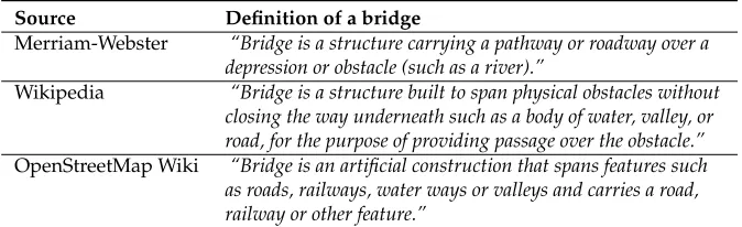
defi-nitions may, however, be incomplete and insufficiently specific, thus interpreted differently by different operators during the manual object classification. For example, the first two definitions both identity the function of a bridge in providing passage over an obstacle (i.e., “carrying a pathway” and “providing passage”). However, the wordobstacleis absent from the third definition where it is only stated that a bridge spans features. Also, it is not completely clear from the third definition that a bridge should provide passage. All the examples of the features carried by a bridge do provide passage, but the term “other feature” may be too open for interpretation by the operators.
Source Definition of a bridge
Merriam-Webster “Bridge is a structure carrying a pathway or roadway over a depression or obstacle (such as a river).”
Wikipedia “Bridge is a structure built to span physical obstacles without closing the way underneath such as a body of water, valley, or road, for the purpose of providing passage over the obstacle.”
OpenStreetMap Wiki “Bridge is an artificial construction that spans features such as roads, railways, water ways or valleys and carries a road, railway or other feature.”
Table 1: Alternative definitions of abridge.
The underlying assumption for a data-driven approach to learn object classifications is that the majority of objects in the dataset is classified correctly. Here, we assume that topological relations between objects can be mined for patterns that occur frequently. Thus, if the majority of objects of a class frequently satisfy the same topological relationship with other objects, this pattern can be learned and used to classify further spatial objects. For example, if the majority of roads in the dataset are connected to other line objects (e.g., other roads), then this pattern can be adapted as a rule. Thus, if there are some roads that are not connected to any other linear objects, they would be seen as potentially erroneous and should be inspected. In this study, we assume that there is one dominant pattern of topological relations for a given object class. Nonetheless, there may be cases where the object class is a generalization of multiple sub-classes with highly distinct patterns. In such cases, defining the entire object class based on only one pattern may be too general. However, this non-trivial problem of detecting aggregate classes of objects (e.g.,transport infrastructure) based on detected patterns is not in the scope of this paper, and may be addressed in future studies.
To realize the stated assumption, it is necessary to identify a model of topological rela-tionships that is expressive enough to capture the functional characteristics of the classes to which it is applied. In this study, we focus on the case of linear objects connected in a network structure (such as a road network) and the topological relationships that can capture the functional distinction between standard road segments and bridges or other structures facilitating carrying over of structures.
3.1
Model of refined topological relations for line objects
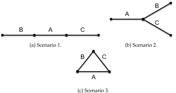
exactly one point with objectA. Furthermore, topological relations betweenAandB or Chave the same 9IM representation in all cases from Figure 1—meets (Table 2a). Table 2c shows the topological relations between objectsA,B, andC in all three scenarios. From the first two columns of that table, it can be seen that these topological scenarios cannot be distinguished using only the 9IM representation of the topological relationships between {A,B} and {A,C}. On the other hand, if the topological relations between {B,C} were also considered, the 9IM could show that scenarios 1 and 2 are topologically different. How-ever, in this case scenario 3 would be identical to scenario 2 and different from scenario 1 (Table 2c). IfAwas an object such as a bridge or a tunnel, the important distinction between these cases would be to capture the connectivity to other objects such as road segmentson both sides, and the given examples show that the 9IM is not able to do that. Thus, this paper first proposes a refinement of the 9IM for linear objects beyond binary relations.
(a) Scenario 1. (b) Scenario 2.
(c) Scenario 3.
Figure 1: Three topological scenarios between three line objectsA,B, andC.
Interior Boundary Exterior Interior F F T
Boundary F T T
Exterior T T T (a) 9IM for the topological relationmeets.
Interior Boundary Exterior Interior F F T
Boundary F F T
Exterior T T T (b) 9IM for the topological relationdisjoint.
Scenario 1 Scenario 2 Scenario 3 A and B meets meets meets
A and C meets meets meets
B and C disjoint meets meets (c) Topological relations between objects in three topological scenarios from Figure 1.
3.2
Computing refined topological relations of line objects
The purpose of this refined model is to find out if the topological relations between acore object with line geometry and otherperipheralobjects are symmetrical (i.e., present on both sides, like in Figures 1a and 1c) or asymmetrical (i.e., present only on one side of the line, like in Figure 1b). In this study, symmetry is only defined and tested for peripheral objects which are topologically related to the end points of the core object (i.e., is not defined for a peripheral line crossing the core object). Also, we do not make any further claims of the mathematical properties of this model (e.g., homeomorphism). Applied in combination, Algorithm 1andAlgorithm 21enable us to capture the relationships between more than two
non-disjoint objects through their refined topological relation.
The goal of Algorithm 1 is to compute the topological relation between the core object and a single peripheral object in a way that shows if the peripheral object is connected to the the start point or the end point of the core object. It requires a single core line object and a single peripheral object as input (e.g., objectsAandBfrom Figure 1). Although the core object may have many peripheral objects, Algorithm 1 only considers one peripheral object at a time, and ought to be run separately for all peripheral objects. Let the geometry of the core object be calledgeom1, and the geometry of the peripheral object be calledgeom2. First, the 9IM relation betweengeom1 and geom2 is calculated. Then, the 9IM relations between each of thegeom1’s boundary points (the start and end point of a line constitute its boundary) andgeom2 are calculated. These steps produce three topological relations which are used as input in the Algorithm 1; one betweengeom1andgeom2(i.e.,RELin Algorithm 1), one between the start point ofgeom1and geom2(i.e., RS in Algorithm 1), and one between the end point ofgeom1andgeom2(i.e.,RE in Algorithm 1). In this paper, the start and end points of the core line object do not relate to its direction, but are terms used only to differentiate the line object’s two extremes. They are extracted directly from the geometry of the line object in the OSM and are usually determined at the time when geometry is created (i.e., the first point of the geometry that user enters will be its start point, and the last entered point will be its end point). Thus, the approach proposed here differs from approaches based on directed line segments [27], or oriented regions [28] that are often used for modelling movement trajectories.
Next, these three topological relations need to be conflated into one topological relation betweengeom1andgeom2, which also distinguishes the side ofgeom1thatgeom2is related to. Unlike line geometries, point geometries do not have a boundary. If a point geometry is related to another geometry, its interior must be related to that other geometry (for more examples and specifics of topological relations with different geometries see [33]). As a result, in the last two topological relations above, only the parts of the 9IM that consider the interior of the point are considered. As shown in Table 2a, this information is usually contained in the first three elements (i.e., first row) of the 9IM (Algorithm 1 line 1).
For the first three values in the 9IM between the start point ofgeom1andgeom2,Tvalues are substituted withS to denote that geom2is topologically related to the start point of geom1. Similarly, in the 9IM for the end point ofgeom1,Tvalues are substituted withE. As a result, topological relations between start and end point ofgeom1andgeom2are now each represented with three values that show if the interior of the point is related to the interior, boundary, and exterior ofgeom2(Algorithm 1 lines 2-3).
To combine these relations into one relation, each of the three values in relation for the start point ofgeom1andgeom2is compared to the corresponding value in the relation between the end point of geom1 and geom2 (Algorithm 1 lines 6-16). If both values are negative (FF), this means that neither the start nor the end point ofgeom1 intersect the interior, boundary, or exterior of geom2). Thus, F is returned as a value for the unified relation in this case. If values areSF, only the start point of geom1 is related to geom2, and Sis returned. Accordingly, if values areFE, only the end point of geom1is related, and E is returned. Finally, values SEmean that both start and end point of geom1 are related togeom2, and Bis returned into the unified relation. At this point, a three-value representation of the topological relationship between the start and end point ofgeom1and geom2is available. This representation is finally used to replace the values in the standard 9IM betweengeom1andgeom2that regard the boundary ofgeom1(Algorithm 1 lines 20-21). These values are usually in the second row of the 9IM matrix (Table 2a).
Algorithm 1Refined topological relations for line objects.
Require: A line geometry (geom1) of one object from the class that is being analyzed (e.g., bridge), and a line or polygon geometry of another object (geom2)
Input:REL←relate_9IM(geom1, geom2),RS←relate_9IM(start_point(geom1), geom2),
RE←relate_9IM(end_point(geom1), geom2)
1: InRSandRE, keep only the 3 values that regard the relations between the points’ interiors and the other object
2: Change all positive (True) values in RS to ‘S’ in order to denote that this relation refers to start point 3: Change all positive (True) values in RE to ‘E’ in order to denote that this relation refers to end point 4:i←0
5:result←“”
6:whilei≤3do 7: x=RS[i] +RE[i]
8: ifx=FFthen
9: y←F
10: else ifx=SFthen
11: y←S
12: else ifx=FEthen
13: y←E
14: else ifx=SEthen
15: y←B
16: end if
17: result←result+y
18: i←i+ 1
19: end while
20: InREL, replace the values regarding the boundary of geom1 with result—a combination of relations between start point of geom1 with geom2, and end point of geom1 with geom2
21: REL[3 : 6]←result
22: ReturnREL
Algorithm 2 shows the second step of the 9IM refinement. Here, the topological rela-tions between the core object and all the peripheral objects in the dataset have already been analyzed with Algorithm 1. The goal of Algorithm 2 is to analyze these relations in order to see if they are symmetrical for the core object.
opposite side of the core object. To test this, when a relation containsSor E, its reverse relation is calculated. This is done by substituting all occurrences ofSin a relation with E, and by substituting all the occurrences ofEwithSin order to construct the same exact topological relation but touching the other point of the core object’s boundary (Algorithm 2 lines 3-4). Then if the reverse relation is also present in the relations that the core object has with other peripheral objects, it can be concluded that the relation is symmetrical.
If a relation is present on both sides of the core object, it gains a suffixboth. On the other hand, if a relation is present only on one side of the core object, it is added a suffix single(Algorithm 2 lines 5-14). It is important to note that the ordering of the start and end point is determined by the order in which the points are inserted when the geometry is being created. Because of this, start and end point do not have any semantic meaning and in practice depend on the order of data entry. In this model, they are used only to ascertain the existence of a relation on both sides of the core object.
Algorithm 2Grouping refined topological relations for a line object.
Require:A set of all topological relations that one line object has with other objects, where topological relations are represented as refined topological relations for line objects as per Algorithm 1
1: result←[]
2: forrelationinrelationsdo
3: ifSinrelationandEinrelationthen
4: Calculate the reverse relation by replacing all occurrences ofSin relation withE, and by replacing all occurrences ofEin relation withS
5: ifreverseinrelationsthen
6: Replace all occurrences ofEandSin reverse relation withT 7: reverse_relation=reverse_relation+-both
8: result=result+reverse_relation
9: Delete the first occurrence ofreverse_relationinrelationsarray 10: else
11: Replace all occurrences ofEandSin reverse relation withT 12: reverse_relation=reverse_relation+-single 13: result=result+reverse_relation
14: end if 15: else
16: result=result+relation
17: end if 18:end for 19:Returnresult
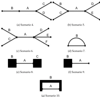
(a) Scenario 4. (b) Scenario 5.
(c) Scenario 6. (d) Scenario 7.
(e) Scenario 8. (f) Scenario 9.
(g) Scenario 10.
Figure 2: Two topological scenarios between three line objectsA,B, andC.
4
Discovering object classes by topological relationships
The proposed data-driven approach for object classification has the advantage of not re-lying on human interpretation of a class definition. In this paper, the learned frequent patterns in topological relationships among spatial objects are called themodel.
As the model is learned based on all labelled instances of a class, it operationalizes an extensional definition of an object class [29]. This can also be seen as a data-driven or bottom-up approach [34], which differs from intensional definitions that are formalized prior to object creation and classify objects based on their alignment with the definition (e.g., definitions from Table 1).
Scenario 9IM Algorithm 1 Algorithm 2
Figure 1a FFTFTTTTT,FFTFTTTTT FFTFSETTT,FFTFESTTT FFTFTTTTT-both
Figure 1b FFTFTTTTT,FFTFTTTTT FFTFESTTT,FFTFESTTT FFTFTTTTT-single, FFTFTTTTT-single
Figure 1c FFTFTTTTT,FFTFTTTTT FFTFSETTT,FFTFESTTT FFTFTTTTT-both
Figure 2a FFTFTTTTT,FFTFTTTTT FFTFTTTTT
FFTFSETTT,FFTFESTTT FFTFESTTT
FFTFTTTTT-both, FFTFTTTTT-single
Figure 2b FFTFTTTTT,FFTFTTTTT FFTFTTTTT,FFTFTTTTT
FFTFSETTT,FFTFSETTT
FFTFESTTT,FFTFESTTT
FFTFTTTTT-both,
FFTFTTTTT-both
Figure 2c FFTFTTTTT,FFTFTTTTT, FFTFTTTTT,FFTFTTTTT, FFTFTTTTT FFTFSETTT,FFTFSETTT, FFTFESTTT,FFTFESTTT, FFTFESTTT FFTFTTTTT-both, FFTFTTTTT-both, FFTFTTTTT-single
Figure 2d FFTFTFTFT FFTFBFTFT FFTFBFTFT
Figure 2e FFTFTTTTT,FFTFTTTTT FFTFSETTT,FFTFESTTT FFTFTTTTT-both
Figure 2f FFTFTTTTT FFTFSETTT FFTFTTTTT-single
Figure 2g FFTFTFTTT FFTFBFTTT FFTFBFTTT
Table 3: Topological relations between objectAand other objects in Figure 1 represented with the 9IM, Algorithm 1, and Algorithm 2.
in the contingency table show how real-world features should be classified, while the rows show how the corresponding data are actually classified in the dataset.
Ground truth
class not class
Dataset class T P F P
not class F N T N
(a) Ground truth vs. Dataset.
Model
class not class
Dataset class T P F P
not class F N T N
(b) Dataset vs. Model.
Table 4: Variants of contingency tables comparing data against ground truth or against a model, respectively. True positives (TP) are objects that are correctly classified, false pos-itives (FP) are objects which have been classified into a class incorrectly. False negatives (FN) are objects that have been omitted, and true negatives (TN) are objects that have been correctly classified as not part of a given class.
On the other hand, the approach proposed in this paper compares the existing classifi-cation to the classificlassifi-cation performed by the model, as shown in Table 4b. It is important to note that the proposed approach uses only the objects that are classified into the given class (i.e., first row of Table 4a) for learning the model. This enables it to be used in cases when ground truth is not available.
The other type is when objects should belong to the given class in the data, but they do not. These are errors by omission and correspond toFNin Table 4b.
However, the detected errors do not always have to be caused by incorrect classification, and the issue does not have to be caused by the core object that is being analyzed. For example, a bridge object that does not cross any peripheral objects in the data may be caused by the misplacement of the peripheral object in the data (e.g., a river is misplaced in the data), by the misplacement of the bridge in the data, or by the absence of the obstacle object from the data due to the incompleteness (e.g., a river is missing from the data) or the obstacle object being out of the scope of the dataset (e.g., terrain depressions may be crossed by bridges and not present in the data).
4.1
Approach
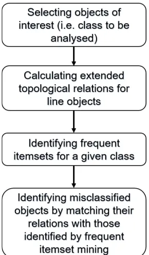
This paper proposes a methodology that mines topological relations for a given object class using the frequent itemset mining method [1] to learn the most frequent topological rela-tions that the objects of that class have with other objects in the dataset. Figure 3 shows a flowchart containing the steps of the proposed method.
Figure 3: Steps of the proposed method.
The first step in this approach is to select objects of interest from a spatial dataset—these will represent the set of core objects. For example, in the case study presented in Section 5, all the instances of the classbridgein a spatial dataset are selected as core objects.
relations for line objects proposed in Section 3. Only the peripheral objects that are not disjoint from the core object have been considered. Since these topological relations are the input of the frequent itemset mining process, this step can be seen as feature engineering.
Finally, for each of the selected core objects, their topological relations with peripheral objects are analyzed to extract the most frequently occurring topological relations. This enables automated inference of principal topological constraints for the class of objects of interest.
4.2
Frequent itemset mining
We aim to learn which topological relations occur frequently among spatial objects of a given class. This is a typicalfrequent itemset miningtask and can be achieved by retrieving the topological relations for the objects of interest and mining the recurrent topological pat-terns among them. Frequent itemset mining is the first step in the association rule mining process, aiming to identify associations between items in transactions [1]. In a database, a transaction usually corresponds to a row and items in a transaction correspond to column cells in a row. The aim is to find a set of items that frequently appear together [7].
Let a set B = {i1, . . . , im} of items be called the item base, and a database T = {t1, . . . , tn}containing transactions. In this case item baseBcontains all items that occur in
databaseT. The term itemset refers to any subset ofBand can be denoted asI⊆B. A typ-ical way to express how frequently an itemset occurs in the database is through computing thesupportof an itemset. The support of the itemsetIis the number of transactions, i.e., tj,1≤j≤n, inTthat contain itemsetI. It can also be expressed as the ratio of transactions
that containIto all transactions inT [7].
The proposed approach adopts the a priori algorithm [1] to find the frequent itemsets in the dataset. There is no constraint set on the length of itemsets that should be retrieved, and the only threshold used is the minimum support of an itemset. In this study:
• itemsare topological relations that objects of a given class have with other objects in the database, and which are expressed using the refined topological relations for line objects,
• transactionsare rows of a database table where one row contains all topological rela-tions between a core object and peripheral objects in the database (i.e., there is exactly one transaction for each core object), and
• itemsetsare sets of topological relations that occur together in the same transaction, i.e., for one core object.
Figure 4: Examples of bridges and their topological relations with other objects.
Topological relations Bridge Member relations
1 meets, crosses, meets 2 meets, crosses, meets, meets 3 meets, meets
(a) Dataset transactions consisting of topological relations.
Frequent itemsets Itemset Support (meets) 3/3 = 100% (crosses) 2/3 = 66% (meets, crosses) 2/3 = 66%
(b) Frequent itemsets and their supports.
Table 5: Dataset transactions consisting of topological relations (left), and frequent itemsets and their supports (right) for examples of bridges shown in Figure 4.
5
Case study on bridges in OSM
To evaluate the proposed method, we considerbridgeobjects in the OpenStreetMap (OSM) dataset. In the case study, all the instances of classbridgeare analyzed to learn their most frequent topological relations with their surrounding objects. Apart from the topological relations themselves, the different types of geometry of the peripheral objects (i.e., line or polygon) are distinguished as well. Thus, results are shown in the form of frequent itemsets that consist of topological relations between bridges as core objects and peripheral objects, together with corresponding supports.
5.1
Dataset and experimental setup
We extracted raw OSM data for the State of Victoria, Australia through the OSMOverpass API2. The experimental setup consists of aPostgreSQL 9.5.133 database with thePostGIS 2.4.24extension, where OSM data were imported using theosm2pgsql 0.88.15importer.
2http://wiki.openstreetmap.org/wiki/Overpass API 3https://www.postgresql.org/
4http://postgis.net/
A preselection step was used to select bridge objects from the raw data. It was guided by the OSM wiki documentation which specifies that bridges should have a line geometry and should contain abridge=*tag. Thus, objects that were annotated as bridges but did not have a line geometry were excluded from the experiment. Furthermore, objects tagged asbridge=nowere also excluded. Note that this preselection was applied only to identify the set of core objects (bridges) in the dataset. For peripheral objects related to bridges, all objects with a line or polygon geometry were considered. The counts of line objects and bridges in this dataset are shown in Table 6. These counts are used to calculate the support of frequent itemsets and consequently to identify patterns.
Number of line objects 450 230 Number of line objects annotated as bridge 10 870 Number of polygon objects 404 221
Table 6: Numbers of line features and bridges in the OSM dataset for the state of Victoria, Australia.
In order to compare the proposed refined topological relations for line objects to the 9IM, all experiments were evaluated with both representations of topological relations. All topological relations in the results are represented with aliases for improved readability (Table 7), and the illustrations of the topological relations are shown in Figure 5.
Alias Refined topological relations for line objects 9IM meets-linestring-both FFTFTTTTT-linestring-both —
meets-linestring — FFTFTTTTT-linestring
crosses-linestring TFTFFBTTT-linestring TFTFFTTTT-linestring within-polygon TFFBFFTTT-polygon TFFTFFTTT-polygon
Table 7: Aliases used for topological relations in the results.
(a) meets-linestring-both (b) meets-linestring
(c) crosses-linestring (d) within-polygon
5.2
Support threshold for frequent itemsets
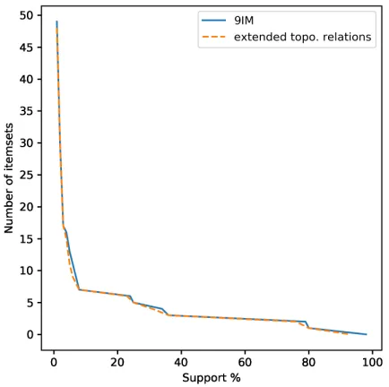
The minimum support threshold for discovery of the frequent itemsets has been set to 20% in this case study. This threshold was empirically determined – larger thresholds lead to frequent itemsets that are too specific, while smaller thresholds yield uninformative item-sets. Figure 6 shows how the number of itemsets diminishes with the increase of the min-imum support threshold. At the threshold of 1%, both 9IM and the refined topological relations for line objects yield almost 50 itemsets, most of which have support lower than 5%. Also, if the threshold was set to 0.001%, there would be almost2 000possible itemsets. On the other side, thresholds of approximately 40% and higher yield less than five itemsets, and the highest possible threshold that would yield at least one itemset would be approx-imately 90%. Thus, given the assumption of this study that we want to learn the patterns of the majority of the data (i.e., those would be patterns with support of at least 50%), it can be concluded that the 20% threshold provides the best balance between specificity and accuracy of the itemsets.
Figure 6: Numbers of the discovered frequent itemsets for different minimum support thresholds, dataset for Victoria.
5.3
Identified frequent itemsets
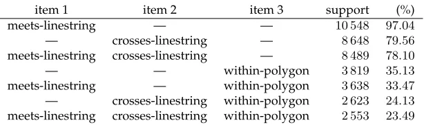
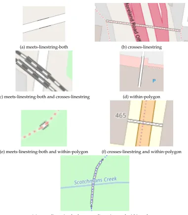
which also have the topological relationcrosses-linestringare also present in row three. Also, the examples of itemsets from Table 9 are shown in Figure 7.
item 1 item 2 item 3 support (%)
meets-linestring — — 10 548 97.04
— crosses-linestring — 8 648 79.56 meets-linestring crosses-linestring — 8 489 78.10 — — within-polygon 3 819 35.13 meets-linestring — within-polygon 3 638 33.47 — crosses-linestring within-polygon 2 623 24.13 meets-linestring crosses-linestring within-polygon 2 553 23.49
Table 8: Frequent itemsets for bridges in the state of Victoria using the 9IM.
item 1 item 2 item 3 support (%)
meets-linestring-both — — 10 001 92.01 — crosses-linestring — 8 649 79.57 meets-linestring-both crosses-linestring — 8 190 75.34
— — within-polygon 3 821 35.15
meets-linestring-both — within-polygon 3 366 30.97 — crosses-linestring within-polygon 2 624 24.14 meets-linestring-both crosses-linestring within-polygon 2 441 22.46
Table 9: Frequent itemsets for bridges in the state of Victoria, using the refined topological relations for line objects.
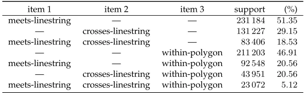
Consecutively, we apply the identified frequent itemsets on all line objects in the dataset. The frequent itemset mining with the same minimum 20% support threshold was applied to all line objects in the dataset (Tables 10 and 11), to identify unclassified or potentially misclassified objects that satisfy the constraints for the classbridge. We thus evaluate how specific the learned topological constraints are to the classbridge. In this step, no preselection other than restricting the set to line objects has been made.
5.4
Results
(a) meets-linestring-both (b) crosses-linestring
(c) meets-linestring-both and crosses-linestring (d) within-polygon
(e) meets-linestring-both and within-polygon (f) crosses-linestring and within-polygon
(g) meets-linestring-both, crosses-linestring, and within-polygon
Figure 7: Examples of the itemsets from Table 9, shown on bridges in OSM.
in the rightmost columns, a feature must have all three topological relations with periph-eral features to be classified as a bridge.
The results have been evaluated with five quality measures:
• Precision: fraction of objects in the dataset classified as bridges by the proposed ap-proach (model) and also classified as bridges in the dataset.
item 1 item 2 item 3 support (%) meets-linestring — — 231 184 51.35 — crosses-linestring — 131 227 29.15 meets-linestring crosses-linestring — 83 406 18.53 — — within-polygon 211 203 46.91 meets-linestring — within-polygon 92 548 20.56 — crosses-linestring within-polygon 43 951 20.56 meets-linestring crosses-linestring within-polygon 23 072 5.12
Table 10: Frequent itemsets for all line objects in the state of Victoria using the 9IM.
item 1 item 2 item 3 support (%)
meets-linestring-both — — 113 095 25.12 — crosses-linestring — 133 634 29.68 meets-linestring-both crosses-linestring — 49 427 10.98 — — within-polygon 218 512 48.53 meets-linestring-both — within-polygon 38 749 8.61
— crosses-linestring within-polygon 44 838 9.959 meets-linestring-both crosses-linestring within-polygon 11 849 2.632
Table 11: Frequent itemsets for all line objects in the state of Victoria, using refined topo-logical relations for line objects.
• Recall: fraction of objects in the dataset that are classified as bridges in the dataset and were also classified as bridges by the proposed approach.
recall= T P T P +F N
• Accuracy: ratio of all the objects that were correctly classified as either bridges or not bridges to all the incorrectly classified objects. It captures how the approach (classifi-cation) compares to the existing classification in the dataset.
accuracy= T P+T N T P +T N+F P +F N
• Specificity: ratio of all objects that were correctly classified as not bridges by the pro-posed method, and all objects that were classified as not bridges in the dataset. It captures how many objects that are not classified as bridges in the dataset have been correctly classified as not bridges by the proposed method.
specif icity= T N T N+F P
• F1 score (less commonly calledSørensen-Dice index): the harmonic mean of precision and recall. This measure is commonly used for evaluation of machine learning clas-sification tasks (for a review, see [35]).
The quality measures for the proposed method using the 9IM are shown in Figure 8a and in Table 14. The same measures for the proposed method using refined topological relations for line objects are shown in Figure 8b and in Table 14. The proposed method was also applied to the OSM dataset for Switzerland in order to test if the method will be general enough to yield similar results elsewhere in the world. The quality assessment of these results is shown in Figure 9.
Data
meets-LineString-both AND crosses-LineString AND within-Polygon bridge not bridge bridge not bridge bridge not bridge
Model bridge 10 548 220 636 8 489 74 917 2 553 20 519 not bridge 322 218 724 2 381 364 443 8 317 418 841
Table 12: Contingency table for the results using the 9IM. AND means that this item is applied in conjunction with the previous item(s) to the left of it in an itemset, applied on the OSM dataset for the state of Victoria.
Data
meets-LineString-both AND crosses-LineString AND within-Polygon bridge not bridge bridge not bridge bridge not bridge
Model bridge 10 001 103 094 8 190 41 237 2 441 9 408 not bridge 869 336 266 2 680 398 123 8 429 429 952
Table 13: Contingency table for the results using refined topological relations for line ob-jects. AND means that this item is applied in conjunction with the previous item(s) to the left of it in an itemset, applied on the OSM dataset for the state of Victoria.
9IM
meets-linestring AND crosses-linestring AND within-polygon
precision 0.0456 0.1018 0.1107
recall 0.9704 0.7810 0.2349
accuracy 0.5092 0.8283 0.9360
specificity 0.4978 0.8295 0.9533
F1 score 0.0872 0.1801 0.1504
Refined topological relations for line objects
meets-linestring-both AND crosses-linestring AND within-polygon
precision 0.0884 0.1657 0.2060
recall 0.9201 0.7535 0.2246
accuracy 0.7691 0.9025 0.9604
specificity 0.7654 0.9061 0.9786
F1 score 0.1614 0.2717 0.2149
(a) The 9IM. (b) Refined topological relations for line objects.
Figure 8: Quality measures for the results using the 9IM and refined topological relations for line objects, applied on the OSM dataset for the state of Victoria.
6
Discussion
Our first observation is that the itemsets discovered in the experiment (Tables 8 and 9) are strongly comparable with the common sense, textual definitions of bridges (Table 1, Section 3). These definitions state that a bridge should carry a path or a road over an obstacle. In the discovered itemsets, the bridge crossing an obstacle is represented with the crosses-linestringrelation. In the OSM dataset, a bridge is also part of the road or pedestrian network, and as such represents a specialization of a road network. This means that a bridge is not only a structure that carries a path or a road, but is the path or the road itself. This is the first, most common item in the itemsets discovered, captured as the meets-linestringrelation.
(a) The 9IM. (b) Refined topological relations for line objects.
Figure 9: Quality of the results using the 9IM and refined topological relations for line objects on the OSM dataset for Switzerland.
yield superior results enabling to identify and verify these marginal cases. A 5% error rate represents around approximately 500 objects just in our limited dataset.
This difference is also present in the results for all line objects (Tables 11 and 10) where many more line objects have the relation meets-linestring (51%), compared to the relationmeets-linsetring-both(25%). This is to be expected because the latter is a proper subset of themeets-linestringrelation set. Yet, it is also insufficiently specific to bridges. This effect propagates through the rest of the itemsets where these relations are present, while the other itemsets have similar support for both representations of topolog-ical relationships.
Evaluation of the results (Figure 8 and Table 14) shows how the quality of the clas-sification changes with different itemsets. The evaluation is performed using three rules—meets-linestring-both, crosses-linestring, and within-polygon— which are being added from left to right with logical operator AND. In the last case, this means that an object needs to have all three relationships with its surrounding objects to be classified as a bridge.
(a) Footway bridge connected on a single side. (b) Cycleway bridge meeting cycleway at a non-break point.
(c) Footway bridge connected on a single side. (d) Road bridges connected on a single side.
Figure 10: Examples of bridges meeting line objects only on one side.
other line objects in the dataset. On the other hand, the precision of the proposed method is low, and just reaches 20% when all three rules are applied. The reason is that many features that are not bridges are committed—incorrectly classified as bridges (Table 13). In other words, these conditions are only necessary for bridges, but are not unique to this class of objects. Figure 11 shows four examples of line objects which are not annotated as bridges in the data, but are classified as bridges by the model because they have topological relationsmeets-linestring-both and crosses-linestring with their peripheral objects. The example in Figure 11a shows a footway that is crossing a stream without a bridge which means that the bridge is possibly missing from the dataset. In Figures 11b and 11d, roads are crossing power-lines and meeting other road segments on both sides which makes them topologically identical to bridges in the model. The example in Fig-ure 11c shows us that the obstacles being crossed by bridges can also have the topological characteristics of a bridge if they are a part of a network (i.e., meeting other line objects on both sides), because they will already have the topological relationcrosses-linestring with the bridge. This problem may be solved by making further implications from seman-tics (i.e., a river is not likely to be a bridge, regardless of its topological relations), or by considering additional attribute information (i.e., taglayer=*is often used in OSM to de-scribe vertical relationships between overlapping objects such as roads). However, this is out of the scope of this paper and will be considered in the future studies.
the low precision. The refined topological relations method outperforms the 9IM by im-proving precision by 6%, accuracy and specificity by 7%, and the F1 score by 9% on the the combination of meets-linestring-both and crosses-linestring. The relative improvement on F1 score with the refined topological relations method is thus 50% over the 9IM-based rules. The 9IM achieves a slightly higher recall by 3%, since the relation meets-linestring is more general than the meets-linestring-both relation. In summary, the overall classification performs best when applying the proposed refined topological relations over the 9IM, with the combination of rules meets-linestring-bothandcrosses-linestring.
(a) Footway classified as a bridge. (b) Road crossing a power-line classified as a bridge.
(c) Road being crossed by bridges (white) classi-fied as a bridge.
(d) Road crossing a power-line and a cycleway classified as a bridge.
Figure 11: Examples of lines incorrectly classified as bridges by the model.
7
Conclusion and future work
in different languages which may also affect their interpretation, and studies have already proposed topology as a solution to these issues [15].
We address these problems based on a hypothesis that topological relationships be-tween spatial objects in large datasets can be analysed automatically to support the clas-sification of spatial objects. We propose an intrinsic approach for automated learning of object classes with frequent itemset mining. We demonstrate that such an approach is able to learn which topological relationships the objects of a given class commonly have with other objects in the dataset, and to express these relationships as topological constraints. The constraints can then be used to classify objects (either on their own or in conjunction with other approaches) or at least verify their classification.
In addition, this paper presents how topology can be used as a defining property for classes of spatial objects (Section 3). Furthermore, problems regarding the 9IM and its abil-ity to show more complex relations, such as whether a line object in a network is connected on both sides to the network, have been discussed. We introduce a refinement of the 9IM for line objects, enabling to distinguish situations if a line object is connected on one or on both sides in topological scenarios that include more than two objects (Figure 1).
The proposed method has been tested on the OSM data for the state of Victoria, Aus-tralia. The aim of this case study is to analyze all objects belonging to the classbridge, and learn which topological relations these objects have with their surrounding objects in the dataset. The proposed approach was able to learn all the rules present in the textual defi-nitions of bridges (Table 1), stating that a bridge should cross an obstacle and carry a path or a road over this obstacle. In addition, by learning these rules directly from the data, the proposed approach shows an additional benefit of recognising that in the OSM model the bridge itself represents a path or a road, rather than carrying it.
The evaluation has showed that the proposed approach is able to perform the classification task at a high standard. Using the meets-linestring-both and crosses-linestringrules, it is able to classify bridges with 90% accuracy, 90% speci-ficity, and 75% recall. However, low precision (17%) is reached since a large number of line objects are incorrectly classified as bridges. Here, the refined topological relations for line objects have outperformed the 9IM in precision, accuracy, specificity, and F1 score by 6%, 7%, 7%, and 9% respectively, while having 3% lower recall. This shows that the proposed method can be successfully used to check the existing classification in the data but has problems when trying to discover errors by omission (i.e., error where an object should be classified as a bridge, but is not).
Overall, success of the case study has justified the plausibility of the proposed method, thus supporting the stated hypothesis. The proposed method contributes an automated way of defining classes of spatial objects, which can improve the classification quality of a dataset and save human effort. The primary utility of our method is that it enables one to efficiently learn class patterns from data, identify possible anomalies in the data, and present anomalous entries to an operator for verification, possibly through a graphical user interface.
pathway). In future studies, the proposed method may be extended with additional ge-ometrical, hierarchical [14], or even attribute properties, enabling to further differentiate classes of objects. Extensions of the proposed method are likely to be of particular interest to classes of objects that assure connectivity across the 3D dimension (i.e., tunnels and other crossings) and objects that assure transitions between environments (e.g., jetties and piers). The challenge lies in defining which properties should be studied, as they may differ be-tween different geometry types. For example, length, number of nodes, angles, and the fact whether a line is open or closed might be interesting geometrical properties of line objects to consider.
Acknowledgments
Support by the Australian Research Council (DP170100153) is acknowledged.
References
[1] AGRAWAL, R., MANNILA, H., SRIKANT, R., TOIVONEN, H., AND VERKAMO, A. I.
Fast discovery of association rules. InAdvances in knowledge discovery and data min-ing, U. M. Fayyad, G. Piatetsky-Shapiro, P. Smyth, and R. Uthurusamy, Eds., vol. 12. American association for artificial intelligence, 1996, pp. 307–328.
[2] ALEXANDROFF, P.Elementary concepts of topology. Dover, New York, NY, USA, 1961.
[3] ALI, A. L., FALOMIR, Z., SCHMID, F., ANDFREKSA, C. Rule-guided human classi-fication of volunteered geographic information. ISPRS journal of photogrammetry and remote sensing 127(2017), 3–15. doi:10.1016/j.isprsjprs.2016.06.003.
[4] ALI, A. L., SCHMID, F., AL-SALMAN, R.,ANDKAUPPINEN, T. Ambiguity and plausi-bility: managing classification quality in volunteered geographic information. In Pro-ceedings of the 22nd ACM SIGSPATIAL international conference on advances in geographic information systems(New York, NY, USA, 2014), SIGSPATIAL ’14, ACM, pp. 143–152. doi:10.1145/2666310.2666392.
[5] ALI, A. L., SCHMID, F., FALOMIR, Z.,ANDFREKSA, C. Towards rule-guided classifi-cation for volunteered geographic information.ISPRS annals of photogrammetry, remote sensing and spatial information sciences II-3/W5(2015), 211–217. doi:10.5194/isprsannals-II-3-W5-211-2015.
[6] BARRON, C., NEIS, P., AND ZIPF, A. A comprehensive framework for intrin-sic OpenStreetMap quality analysis. Transactions in GIS 18, 6 (2014), 877–895. doi:10.1111/tgis.12073.
[7] BORGELT, C. Frequent item set mining.Wiley interdisciplinary reviews: data mining and knowledge discovery 2, 6 (2012), 437–456. doi:10.1002/widm.1074.
[9] BRANDO, C., BUCHER, B., ANDABADIE, N. Specifications for user generated spa-tial content. InAdvancing geoinformation science for a changing world. Lecture notes in geoinformation and cartography, S. Geertman, W. Reinhardt, and F. Toppen, Eds., vol. 1. Springer, Berlin, Heidelberg, Berlin, Heidelberg, 2011, pp. 479–495. doi:10.1007/978-3-642-19789-5_24.
[10] BRAVO, L., AND RODRIGUEZ, M. A. Formalization and reasoning about spa-tial semantic integrity constraints. Data and knowledge engineering 72(2012), 63–82. doi:10.1016/j.datak.2011.09.006.
[11] CLEMENTINI, E., AND DI FELICE, P. A comparison of methods for
represent-ing topological relationships. Information sciences - applications 3, 3 (1995), 149–178. doi:10.1016/1069-0115(94)00033-X.
[12] CLEMENTINI, E.,ANDDIFELICE, P. A model for representing topological relation-ships between complex geometric features in spatial databases.Information sciences 90, 1-4 (1996), 121–136. doi:10.1016/0020-0255(95)00289-8.
[13] CLEMENTINI, E., DIFELICE, P.,AND VANOOSTEROM, P. A small set of formal topo-logical relationships suitable for end-user interaction. InAdvances in spatial databases. SSD 1993. Lecutre notes in computer science (1993), D. Abel and B. Chin Ooi, Eds., vol. 692, Springer, Berlin, Heidelberg, pp. 277–295. doi:10.1007/3-540-56869-7_16.
[14] CORCORAN, P., MOONEY, P., AND BERTOLOTTO, M. Spatial relations using high level concepts. ISPRS international journal of geo-information 1, 3 (2012), 333–350. doi:10.3390/ijgi1030333.
[15] DUBE, M. P., AND EGENHOFER, M. J. An ordering of convex topological rela-tions. InGeographic information science. GIScience 2012. Lecture notes in computer science (Berlin, Heidelberg, 2012), N. Xiao, M.-P. Kwan, M. F. Goodchild, and S. Shekhar, Eds., vol. 7478, Springer, Berlin, Heidelberg, pp. 72–86. doi:10.1007/978-3-642-33024-7_6.
[16] EGENHOFER, M. J., AND FRANZOSA, R. D. Point-set topological spatial rela-tions. International journal of geographical information systems 5, 2 (1991), 161–174. doi:10.1080/02693799108927841.
[17] EGENHOFER, M. J., AND HERRING, J. R. Categorizing binary topological relations
between regions, lines, and points in geographic databases. Tech. rep., University of Maine, National Center for Geographic Information and Analysis and Department of Surveying Engineering, Department of Computer Science, 1990.
[18] EGENHOFER, M. J.,ANDMARK, D. M. Naive geography. InSpatial information theory: a theoretical basis for GIS. COSIT 1995. Lecture notes in computer science(Semmering, Austria, 1995), A. U. Frank and W. Kuhn, Eds., vol. 988, Springer, Berlin, Heidelberg, pp. 1–15. doi:10.1007/3-540-60392-1_1.
[19] GIRRES, J. F., AND TOUYA, G. Quality assessment of the French OpenStreetMap dataset.Transactions in GIS 14, 4 (2010), 435–459. doi:10.1111/j.1467-9671.2010.01203.x.
[21] GRÖGER, G., AND PLÜMER, L. Topology of surfaces modelling bridges and tun-nels in 3D-GIS. Computers, environment and urban systems 35, 3 (2011), 208–216. doi:10.1016/j.compenvurbsys.2010.10.001.
[22] HADZILACOS, T., AND TRYFONA, N. A model for expressing topological integrity constraints in geographic databases. InTheories and methods of spatio-temporal reasoning on theories and methods of spatio-temporal reasoning in geographic space. Lecture notes in computer science, A. U. Frank, I. Campari, and U. Formentini, Eds., vol. 639. Springer, Berlin, Heidelberg, Berlin, Heidelberg, 1992, pp. 252–268. doi:10.1007/3-540-55966-3_15.
[23] HAKLAY, M. M., BASIOUKA, S., ANTONIOU, V., AND ATHER, A. How many volunteers does it take to map an area well? The validity of Linus’ law to vol-unteered geographic information. The cartographic journal 47, 4 (2010), 315–322. doi:10.1179/000870410X12911304958827.
[24] HAN, J., CAI, Y.,ANDCERCONE, N. Knowledge discovery in databases: an attribute-oriented approach. InProceedings of the 18th international conference on very large data bases(San Francisco, CA, USA, 1992), L.-Y. Yuan, Ed., VLDB ’92, Morgan Kaufmann publishers Inc., pp. 547–559.
[25] ISO. ISO 19157:2013: Geographic information—data quality. Tech. rep., 2013.
[26] JILANI, M., CORCORAN, P., ANDBERTOLOTTO, M. Automated highway tag assess-ment of OpenStreetMap road networks. InProceedings of the 22nd ACM SIGSPATIAL international conference on advances in geographic information systems (New York, NY, USA, 2014), SIGSPATIAL ’14, ACM, pp. 449–452. doi:10.1145/2666310.2666476.
[27] KURATA, Y.,AND EGENHOFER, M. J. The 9 + - intersection for topological relations between a directed line segment and a region. InWorkshop on behaviour monitoring and interpretation. BMI ’07(2007), B. Gottfried, Ed., no. 42, TZI-Berichte, pp. 62–76.
[28] LEWIS, J. A., ANDEGENHOFER, M. J. Oriented regions for linearly conceptualized features. InGeographic information science. GIScience 2014. Lecture notes in computer sci-ence(2014), M. Duckham, E. Pebesma, K. Stewart, and A. U. Frank, Eds., vol. 8728, Springer, Cham, pp. 333–348. doi:10.1007/978-3-319-11593-1_22.
[29] MAJIC, I., WINTER, S., AND TOMKO, M. Finding equivalent keys in Open-StreetMap: semantic similarity computation based on extensional definitions. In Proceedings of the 1st workshop on artificial intelligence and deep learning for geographic knowledge discovery (New York, NY, USA, 2017), GeoAI ’17, ACM, pp. 24–32. doi:10.1145/3149808.3149813.
[30] MARK, D. M.,ANDTURK, A. G. Landscape categories in Yindjibarndi: ontology, en-vironment, and language. InSpatial information theory. Foundations of geographic infor-mation science. COSIT 2003. Lecture notes in computer science.(Berlin, Heidelberg, 2003), W. Kuhn, M. F. Worboys, and S. Timpf, Eds., vol. 2825, Springer, Berlin, Heidelberg, pp. 28–45. doi:10.1007/978-3-540-39923-0_3.
M. Duckham, L. Kulik, and B. Kuipers, Eds., vol. 4736, Springer, Berlin, Heidelberg, pp. 285–302. doi:10.1007/978-3-540-74788-8_18.
[32] RANDELL, D. A., CUI, Z., ANDCOHN, A. G. A spatial logic based on regions and connection. InProceedings of the third international conference on principles of knowledge representation and reasoning(San Francisco, CA, USA, 1992), B. Nebel, C. Rich, and W. Swartout, Eds., KR’92, Morgan Kaufmann Publishers Inc., pp. 165–176.
[33] SCHNEIDER, M., AND BEHR, T. Topological relationships between complex spatial objects. ACM transactions on database systems 31, 1 (2006), 39–81. doi:10.1145/1132863.1132865.
[34] SHEEREN, D., MUSTIÈRE, S., AND ZUCKER, J. A data-mining approach for assessing consistency between multiple representations in spatial databases. International journal of geographical information science 23, 8 (2009), 961–992. doi:10.1080/13658810701791949.
[35] SOKOLOVA, M., ANDLAPALME, G. A systematic analysis of performance measures for classification tasks. Information processing & management 45, 4 (2009), 427–437. doi:10.1016/j.ipm.2009.03.002.
[36] VALLIRES, S., BRODEUR, J.,AND PILON, D. Spatial integrity constraints: a tool for improving the internal quality of spatial data. InFundamentals of spatial data quality, R. Devillers and R. Jeansoulin, Eds. John Wiley & Sons, London, UK, 2010, pp. 161– 178. doi:10.1002/9780470612156.ch9.
[37] VANDECASTEELE, A., ANDDEVILLERS, R. Improving volunteered geographic data quality using semantic similarity measurements.International archives of photogramme-try, remote sensing and spatial information sciences XL-2/W1, May 2013 (2013), 143–148. doi:10.5194/isprsarchives-XL-2-W1-143-2013.
[38] ZIELSTRA, D.,ANDZIPF, A. A comparative study of proprietary geodata and