Probability-Model based
Network Traffic Matrix Estimation
Hui Tian1, Yingpeng Sang2, Hong Shen3,4, and Chunyue Zhou1
1 School of Electronics and Information Engineering
Beijing Jiaotong University, China
2
School of Computer Science Beijing Jiaotong University, China
3
School of Information Science and Technology Sun Yat-sen University, China
4 School of Computer Science
University of Adelaide, Australia [email protected]⋆⋆
Abstract. Traffic matrix is of great help in many network applications. However, it is very difficult to estimate the traffic matrix for a large-scale network. This is because the estimation problem from limited link measurements is highly under-constrained. We propose a simple probability model for a large-scale practical net-work. The probability model is then generalized to a general model by including random traffic data. Traffic matrix estimation is then conducted under these two models by two minimization methods. It is shown that the Normalized Root Mean Square Errors of these estimates under our model assumption are very small. For a large-scale network, the traffic matrix estimation methods also perform well. The comparison of two minimization methods shown in the simulation results complies with the analysis.
Keywords:traffic matrix estimation, probability model, NRMSE.
1.
Introduction
In an IP network, the traffic matrix (TM) describes the traffic volumes traversing the network from the input nodes to the exit nodes over a measured period. Such a matrix is very helpful in many network applications such as capacity plan, anomaly detection, traffic engineering, and network reliability analysis [1]. In these application scenarios, TMs act as an important input. The outputs of various network engineering tasks are directly relevant to the input. So plenty of work aim to conduct measurements on TMs [5] or indirect inference from readily available link measurements [15, 16]. Whichever way is used, it is extremely hard to obtain the traffic matrix for a large network.
The link measurements which are related to traffic matrix is more realistic to be
ob-tained in practice. Denote the link measurements byY and the traffic matrix byX.Y
is annl by 1 vector andX isnp by 1 vector wherenl << np. Thus, the relationship
between link measurements and the traffic matrix is represented byY =AXwhereAis
⋆⋆
the routing matrix. Given a set of link measurements, we aim to infer an overall view of the traffic matrix. This is a classic under-constrained, linear-inverse problem. we cannot obtain a solution if we do not introduce any side information such as the prior model of a traffic matrix. Therefore, paper [11, 14] assumed the origin-destination-demands follows a Poisson distribution. In [2], Origin-Destination (OD) pairs are modeled according to a Gaussian distribution. Medina et al. assumed a logit-choice model in [7] and M. Roughan et al. proposed a gravity model [9, 10].
There are plenty of methods proposed based on these prior traffic model assumption such as Bayesian inference, information theoretic approach, maximum likelihood esti-mation, Linear programming and multiresolution analysis method [12]. These methods perform very differently for different traffic data. There is no method which can work well on all traffic data. Compressed Sensing (CS) is recently greatly developed in many applications. It shows that any sufficiently compressible signal can be accurately recov-ered from a small number of non-adaptive, randomized linear projection samples [6]. It can also be applied in traffic matrix estimation due to the sparsity of the traffic matrix such as the work in [3, 4, 8, 17]. In this paper, we look for a sparsity model which can be used for efficient traffic matrix estimation, resulted in a probability model [13]. This model is simple but efficient. From the simulation results, we will see a generalized model based on our probability model can work well in Origin-Destination pair traffic estima-tion. This generalized probability-based model can not only help to generate traffic data for large-scale network simulations, but also help to study sparse traffic matrix.
2.
Model
A large-scale network usually involves multiple routers/switches in multiple levels. In each level, many routers/switches are located for redundancy and reliability. If we sim-plify the network topology without changing basic networking function, we will get a
tree-like network. In the tree-like network, there is one parent node andN children. The
parent node is considered as a node connecting outside Internet and the child nodes are servers which may be composed of a set of children.
Our model starts with a single star network. This star network is assumed to include one parent node and several child nodes which are connected through one router. This star may be the lowest level star and all of similar stars can be aggregated to form the original network. The traffic estimation on this simple star will be formed into the whole network
traffic matrix. By doing so, estimating aN∗Ntraffic matrix by2N link measurements
which is highly under-constrained though, can be largely reduced in the dimensionality of the problem to a simple star network.
We assume a network model which is composed ofnservers which are connected to
the Internet node via 1 router. Given the link measurementsY observed on these edge
links which are immediate link connecting the end nodes, the problem is to estimate the
end-to-end traffic matrixX.Y =AX,Ais annlbynprouting matrix.
In the simple single star model we assume that all servers are the same. We will relax this assumption later on, but this allows us to build a very simple traffic model firstly. This model only needs three probability parameters which is thus named as the probability model. In our probability model, it is assumed any pairs of servers send traffic to each
same probabilityp2and the Internet node sends the traffic to any server with the same
probabilityp3. Obviously,
(n−1)p1+p2= 1, np3= 1. (1)
3.
Traffic matrix estimation
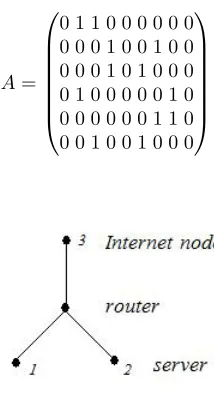
Firstly, we consider a network composed of 2 servers, 1 node denoting Internet and 1
router as Figure 1 shows. Thus we havep1+p2= 1andp3= 1/2. As we consider that a
server will either send the packets to other servers or to the Internet node. There will not
be any traffic to itself. Thus the routing matrixAis
A=
0 1 1 0 0 0 0 0 0 0 0 0 1 0 0 1 0 0 0 0 0 1 0 1 0 0 0 0 1 0 0 0 0 0 1 0 0 0 0 0 0 0 1 1 0 0 0 1 0 0 1 0 0 0
(2)
Fig. 1.A network with 2 servers and 1 Internet node
Assume the total traffic on each node areX′={x′1, x′2, x′3}, wherexi, i∈ {1,2, . . . , n+
1}denotes the total traffic generated by nodei. The elements inY are the traffic on
out-going link from node 1, incoming link to node 1, and then node 2, and 3 with the same order.
Thus,
Y =BX′=
1 0 0 0 p1p3
0 1 0
p1 0 p3
0 0 1
p2p2 0
X′ (3)
Normally we don’t have the full set of the measurements onY. For example, we only
have 3 links’ measurements which is denoted byYs,Ys =BsX′. If we choose 3 links,
node. We denote the selected link measurements asYs, and the selection matrix isBs.
Then we have
Bs=
p01p01pp32
p2p2 0
(4)
Sincedet(Bs) ̸= 0, we haveX′ = B−s1Ys. Because the relationship between the OD
traffic matrixX and traffic generating by end nodesX′can be described by the assumed
probability matrix as follows.
X=P X′ =
0 0 0
p1 0 0
p2 0 0
0 p1 0
0 0 0 0 p2 0
0 0 p3
0 0 p3
0 0 0
X′ (5)
Therefore we haveX =P B−s1Ys.PandBscan both be calculated as above, we can get
a solution toXin this probability model and let it beXp.
Xp=
0 0 0
−1 2 1 2 p1 2p2 −p2
2p1 p2 2p1 1 2 1 2 − 1 2 p1 2p2
0 0 0
p2 2p1
−p2 2p1 1 2 1 2 1 2
−p1 2p2 1
2 1 2
−p1 2p2
0 0 0
Ys (6)
Therefore, we can obtain a solution related to one simple parameter under the
as-sumption of the probability model. Ifp1can be set an appropriate value according to the
realistic networks,Ysis observed measurements on selected links, we can have a
deter-minedXp.
Now our problem is to find a solutionXwhich is the closest toXpunder the constraint
Y =AX. That is,
M inimize f(X) =∥X−Xp∥, s.t. Y =AX,
where∥ · ∥is theL2norm. For simplicity in comparison, we call this to be Minimization
1 (Min 1) method.
This method is difficult to find an efficient solution if there are errors in
measure-ments onY. Therefore, we can employ Lagrangian function. The aim is thus to minimize
L(X, λ).
Again, for simplicity in comparison, we denote this by Min 2 method. In Min 2
method,L2 norm is not easy to write in the form of quadraticX and using derivative,
we solve the problem of
M inimize g(X) =∥X−Xp∥ 2
, s.t. Y =AX,
and construct the Lagrangian function as follows.
L(X, λ) =∥X−Xp∥ 2
+λ∥AX−Y ∥2 (8)
Thus,
L(X, λ) =λXTATAX+λYTY −2λYTAX
+XTX−2XTXp+XpTXp (9)
The Karush-Kuhn-Tucker conditions for this local minimum are given as follows.
∂L(X, λ)
∂X ≥0, (10)
∂L(X, λ)
∂λ = 0, (11)
X∂L(X, λ)
∂λ = 0, (12)
λ∂L(X, λ)
∂λ = 0, (13)
and
X ≥0, λ≥0.
Deriving from above, the KKT conditions are simplified into:
(λATAX+I)X=λATY +Xp, (14)
XTATAX−2YTAX+YTY = 0, (15)
and
X ≥0, λ≥0.
Hereby we can solve this Minimization problem by quadratic programming. Intu-itively, in this quadratic programming, the more links’ measurements are considered, the
4.
Simulations
4.1. Metrics
As we discussed in the above section, there are two regularization methods which obtain
the traffic matrix closest to the matrixXp in the prior assumed model (also called the
probability model). To compare these two methods, we will use Normalized Root Mean Square Error (NRMSE) to show the performance of estimated traffic matrices. Here the
NRMSE is defined ase.
e=
√∑
i( ˆxi−xi) 2
/(N·(N+ 1))
M ax(xi)−M in(xi)
. (16)
Since quadratic distances are acceptable distance metric and lead to simple quadratic opti-mizing problem, it is easy to obtain solutions to both minimization problems. As we have
denoted for simplicity, the Minimization problemM in{d( ˆX, Xp)}subject toY =AX
andX ≥ 0is denoted by Min 1 method and the other Minimization problem by Min 2
method.
Firstly, we simulate both methods on a network withN = 8servers and one Internet
node. Thus in total2(N + 1) = 18links measurements are available. The traffic matrix
to estimate is a 9 by 9 matrix, i.e. an 81 by 1 vector. We obtain a cumulative distribution function (CDF) of NRMSE to observe the performance of these estimates. We then have
a look at the sensitivity of NRMSEs toλ. As the number of links used in measurements
increases, we will check the trend of NRMSEs.
4.2. A General Model
The simple prior model leads to all servers having identical traffic. This may not be accor-dance with the practical cases where there are differences on measurements to different servers. We thus generalize the above simple model to a more practical model which com-bines this simple model with a random traffic model. This general model is described to be
Xgen=αXp+ (1−α)Xrandom.
In this general model, it is seen that the parameterαdefines a random traffic matrix
to be estimated which is still related to the prior assumed probability model. The changes
ofαgive different weights of the prior model in this general model. Intuitively, we can
conclude that the performance of estimates would be affected by this parameterα. Our
simulation will check how NRMSE differs asαincreases. We also introduce a bias factor
β which counts the ratio of wrong measurements to correct measurements. This factor
is helpful in testing the performance of estimation in both the probability model and the general model.
4.3. Experiments
The Figure 2(a) is obtained by monitoring 10 links’ measurements. The other two
estimates by two minimization methods in two models separately. As shown in Figure 2(a), the CDF of NRMSE of estimated results by Min 2 method (represented by two red curves) are worse than that by Min 1 method. However Min 2 method gives very small NRMSE whose CDF approaches to 1 with an NRMSE of 0.045 in the general model. In the probability model, both methods work very competitively and Min 1 is only a bit better than Min 2 method. We also note that by using Min 2 method, the estimation pro-cess gives a much better performance in the probability model than in the general model. Min 1 method does not show this superiority in probability model to general model which shall be shown in a more large-scale network.
Figure 2(b) shows the results when using the full set of 18 links to estimate the original traffic matrix. It is obvious both methods work out CDFs approaching to 1 with smaller NRMSEs, especially when we look at the performance of Min 2 method in the general model. In the probability model, Min 2 method works slightly better than Min 1 method.
This is because more links measurements give more constraints inY =AXwhich limits
the searching space of finding a minimal distance from Xˆ toXp. This outperformance
will be more obvious when there are errors in measurements. This also gives the reason that we prefer Min 2 method to Min 1 method in a large-scale network with more possible errors in measurements.
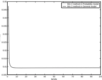
Now we have a look at how NRMSE varies asλincreases when using Min 2 method.
Again, we use measurements on 10 links in this 9-node network simulation and letα=
0.5. Figure 3 shows that the NRMSE does not change whenλtakes a value greater than
a threshold. It is foundλdoes not affect the estimation performance if it is set a value
greater than 5. Therefore, the value ofλbeing 10 in above simulations provides a good
initialization for the traffic estimation process to run.
In the general model,αis a parameter which adjusts the weights of the traffic data
under the probability model assumption and the random traffic data. Figure 4(a) shows
how this parameter affects the performance of estimation. It is obvious that asαincreases
which means the random data weights less, both methods work better. In Figure 4 (a), since all measurements are correct, both methods can work out the same TM which is closest to the practical TM. The curves of both methods are overlapped. When there are errors in measurements, two methods have different performances. We set the bias factor to be 0.1 in Figure 4(b), that is, there are 10% links which have errors in measurements. Min 2 method shows a better performance than Min 1 method. When the bias factor increases which means there are more errors in measurements, the outperformance of Min 2 method to Min 1 method shall be greater.
In Figure 5, the read curve denoted by data 1 gives the result of Min 2 method in the general model. As the number of links used in estimation increases, data 1 shows an improved estimation performance of Min 2 method in the general model. The other three cases do not show obvious change as the number of links used in estimation varies. It is predicted in a large-scale network, using more link measurements would be more beneficial except the case where Min 1 method is used and errors in measurements exist. In practice, the network size is much larger than the above 9-node network simulated
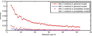
above. How will these two estimation methods perform as the network sizeN is
increas-ing? Figure 6 gives the normalized RMSE by two methods in two models asN changes.
We letα= 0.5,λ= 10and the number of links used to estimate be three. Network size
0 0.01 0.02 0.03 0.04 0.05 0.06 0
0.1 0.2 0.3 0.4 0.5 0.6 0.7 0.8 0.9 1
NRMSE
CDF of NRMSE
Min 2 in general model Min 1 in general model Min 2 in probability model Min 1 in probability model
(a)
0 0.005 0.01 0.015 0.02 0.025 0.03 0.035 0.04 0.045
0 0.1 0.2 0.3 0.4 0.5 0.6 0.7 0.8 0.9 1
CDF of NRMSE
NRMSE
Min 2 in general model Min 1 in general model Min 2 in probability model Min 1 in probability model
(b)
Fig. 2.CDF of Normalized Root Mean Square Error by using both Minimization methods for two models in a 9-node network
0 10 20 30 40 50 60 70 80 90 100
0.005 0.01 0.015 0.02 0.025 0.03 0.035 0.04 0.045 0.05
lamda
NRMSE
Min 2 method in Probability model Min 2 method in General model
0 0.2 0.4 0.6 0.8 1 0
0.1 0.2 0.3 0.4 0.5 0.6 0.7 0.8 0.9 1
alpha
NRMSE
Min2 method Min1 method
(a)
0 0.2 0.4 0.6 0.8 1
0 0.1 0.2 0.3 0.4 0.5 0.6 0.7 0.8 0.9 1
alpha
NRMSE
Min2 method Min1 method
(b)
0 2 4 6 8 10 12 14 16 18 0
0.02 0.04 0.06 0.08 0.1 0.12 0.14 0.16 0.18
Number of links used in estimation
NRMSE
data 1 data 2 data 3 data 4
Fig. 5.Normalized Root Mean Square Error as the number of links used in estimation varies by two methods in two different models
trends to be smaller as the network size increases. Therefore, we can predict when the network size is greater, say hundreds or thousands, the NRMSE of these two estimation methods would work fairly well. Figure 6 also shows two methods work better in prob-ability model than in general model. As we only use 3 links to estimate the total traffic matrix, Min 1 method performs a bit better than Min 2 method. When we have more links’ measurements, Min 2 will show its superiority to Min 1 method as shown in above simulation. Note also both methods work well and are convergent when only 3 links are used in estimation. When there are more links’ measurements available, both methods will perform better.
0 10 20 30 40 50 60
0 0.02 0.04 0.06 0.08 0.1 0.12
Network size N
NRMSE
Min 2 method in general model Min 1 method in general model Min 2 method in probability model Min 1 method in probability model
Fig. 6.Normalized Root Mean Square Error asNchanges by two methods in two different models
5.
Conclusion
star-like networks together to form a large-scale practical network. In order to enable the probability model to adapt to more realistic data in the network, we generalize the proba-bility model to include the random traffic data. Traffic matrix estimation is then conducted under these two models by two minimization methods. It is shown that the Normalized Root Mean Square Errors of these estimates under our model assumption are very small. For a large-scale network, the traffic matrix estimation methods also perform well. The comparisons between two minimization methods showed that Min 2 method is more ro-bust to network measurements errors and thus preferred in practice.
Acknowledgments.This work is supported by National Natural Science Foundation of China No. 61100218 and 61170232, the Fundamental Research Funds for the Central Universities No. 2011JBM206 and No. 2011JBM012, and Beijing Natural Science Foundation No. 4122056.
References
1. Alderson, D.L., Chang, H., Roughan, M., Uhlig, S., Willinger, W.: The many facets of internet topology and traffic. Networks and Heterogeneous Media 1(4), 569–600 (Dec 2006)
2. Cao, J., Davis, D., Wiel, S.V., Yu, B.: Time-varying network tomography. J. Amer. Statis. Assoc 95(452), 1063–1075 (2000)
3. Coates, M., Pointurier, Y., Rabbat, M.: Compressed network monitoring for ip and all-optical networks. In: ACM SIGCOMM Internet Measurement Conference (IMC). pp. 241–252 (2007) 4. Crovella, M., Kolaczyk, E.: Graph wavelets for spatial traffic analysis. In: Proc. of IEEE
Info-com. pp. 1848–1857 (2003)
5. Feldmann, A., Greenberg, A., Lund, C., Reingold, N., Rexford, J., True, F.: Deriving traffic demands for operational ip networks: Methodology and experience. IEEE/ACM Transactions on Networking pp. 265–179 (Jun 2001)
6. Haupt, J., Bajwa, W.U., Rabbat, M., Nowak, R.: Compressed sensing for networked data (Dec 2007)
7. Medina, A., Taft, N., Salamatian, K., Bhattacharyya, S., Diot, C.: Traffic matrix estimation: existing techniques and new directions. SIGCOMM Comput. Commun. Rev. 32(4), 161–174 (2002)
8. Rincon, D., Roughan, M., Willinger, W.: Towards a meaningful mra analysis of traffic matrices. In: ACM SIGCOMM Internet Measurement Conference. pp. 331–336. Vouliagmeni, Greece (Oct 20-22 2008)
9. Roughan, M., Greenberg, A., Kalmanek, C., Rumsewicz, M., Yates, J., Zhang, Y.: Experience in measuring internet backbone traffic variability: Models, metrics, measurements and mean-ing. In: Proc. of the International Teletrafic Congress (ITC-18). pp. 379–388. Berlin Germany (2003)
10. Roughan, M., Thorup, M., Zhang, Y.: Traffic egnieeging with estimated traffic trsffic matrices. In: Proc. ACM SIGCOMM Internet Measurement Conference (IMC). pp. 248–258. Miami Beach, FL, USA (2003)
11. Tebaldi, C., West, M.: Bayesian inference on network traffic using link count data. J. Am. Statist. Assoc. 93(442), 557–576 (1998)
12. Tian, H., Roughan, M., Sang, Y., Shen, H.: Diffusion wavelets-based analysis on traffic matri-ces. In: Proc. of 12th International Conference on Parallel and Distributed Computing, Appli-cations and Technologies. Gwangju, South Korea (Oct 20-22, 2011)
13. Tian, H., Sang, Y., Shen, H.: New methods for network traffic matrix estimation based on a probability model. In: Proc. of IEEE conference on Networks. Singapore (Dec 2011)
15. Zhang, Y., Roughan, M., Duffield, N., Greenberg, A.: Fast accurate computation of large-scale ip traffic matrices from link loads. In: Proc. of ACM SIGMETRICS. pp. 206–217. San Diego, California (Jun 2003)
16. Zhang, Y., Roughan, M., Lund, C., Donoho, D.: An information-theoretic approach to traffic matrix estimation. In: ACM SIGCOMM. pp. 301–312. Karlsruhe, Germany (Aug 2003) 17. Zhang, Y., Roughan, M., Willinger, W., Qiu, L.: Spatio-temporal compressive sensing and
in-ternet traffic matrices. In: Proc. of ACM Sigcomm. pp. 267–278. Barcellona (August 2009)
Hui Tianreceived B. Eng. and M. Eng. degrees from Xidian University, China and Ph.D. from Japan Advanced Institute of Science and Technology, Japan with full-scholarship supported, and awarded ”Excellent Ph.D Gradulate”. She worked in Manchester Metropoli-tan University as a lecturer, and University of Adelaide as a research fellow. She is now an associate professor in Beijing Jiaotong University. Her main research interests include wireless communications and networking, Network Tomography and performance evalu-ation.
Yingpeng Sangreceived the BS degree in computer science from Southwest Jiaotong University, China, in 2001MS degree in computer science from Institute of Mobile Com-munications, Southwest Jiaotong University, in 2004, and PhD degree in computer science from Japan Advance Institute of Science and Technology, in 2007. He is currently an as-sociate professor in Beijing Jiaotong University. His research interests include privacy-preserving problems in databases, data mining and other networking scenarios.
Hong Shenis Professor (Chair) of Computer Science in the University of Adelaide, Aus-tralia, and also a specially appointed professor in Beijing Jiaotong Univeristy. He received the B.E. degree from Beijing University of Science and Technology, M.E. degree from University of Science and Technology of China, Ph.Lic. and Ph.D. degrees from Abo Akademi University, Finland, all in Computer Science. He was Professor and Chair of the Computer Networks Laboratory in Japan Advanced Institute of Science and Technology (JAIST), and Professor (Chair) of Compute Science at Griffith University, Australia. With main research interests in parallel and distributed computing, algorithms, data mining, high performance networks and multimedia systems, he has published more than 200 pa-pers including over 100 papa-pers in international journals such as a variety of IEEE/ACM transactions.
Chunyue Zhoureceived her Ph.D from Beijing Jiaotong University and is now a senior Engineer in Beijing Jiaotong University. Her research interests include the next generation of Internet and information security.