Solutions to the Chinese Postman Problem

California State University, San Bernardino California State University, San Bernardino

CSUSB ScholarWorks

CSUSB ScholarWorks

Theses Digitization Project John M. Pfau Library

2000

Solutions to the Chinese Postman Problem

Solutions to the Chinese Postman Problem

Kenneth Peter Cramm

Follow this and additional works at: https://scholarworks.lib.csusb.edu/etd-project Part of the Algebra Commons

Recommended Citation Recommended Citation

Cramm, Kenneth Peter, "Solutions to the Chinese Postman Problem" (2000). Theses Digitization Project. 1683.

https://scholarworks.lib.csusb.edu/etd-project/1683

SOLUTIONS TO THE CHINESE POSTMAN PROBLEM

A Project

Presented to the

Faculty of

California State University,

San Bernardino

In Partial Fulfillment

of the Requirements for the Degree

Master of Arts ■ < . . in

Mathematics

by ,

Kenneth Peter Cramm

SOLUTIONS TO THE CHINESE POSTMAN PROBLEM

A Project

Presented to the

Faculty of

California State University,

San Bernardino

by

Kenneth Peter Crairan

December 2000

Approved by;

Holland Trapp, Conmittee Chair

Chetan Prakash, Committee Member

Charles Stanton, Chair

Department of Mathematics

I '^/i/on

Date

oseph Chavez,/vommittee Member

J- i 'H"

Terry Hallet,

Graduate Coordinator

Department of

ABSTRACT

We consider the Chinese Postman Problem, in which a mailman

must deliver mail to houses in a neighborhood. The mailman

must cover each side of the street that has houses, at least

once. The focus of this paper is our attempt to discover the optimal path, or the least number of times each street is walked. The integration of algorithms from graph theory and operations research form the method used to explain

solutions to the Chinese Postman Problem.

ACKNOWLEDGMENTS

I thank Jesus Christ, Lord and Savior of the World, for the

intellect to explore the fascinating world of Mathematics.

I thank my wife Carolyn, for her sacrifice of too many

weekends and evenings in order that I may chase after one of

my life's dreams.

I thank my mentor Dr. Roland Trapp, for his youthful

enthusiasm and approach to Mathematics. I will emulate him

in my own attempt to teach students.

TABLE OF CONTENTS

ABSTRACT . . . .. . . . • . . . . - m IV ACKNOWLEDGMENTS

vi

LIST OF TABLES .

vii LIST OF FIGURES

1 INTRODUCTION . ,

5 CHAPTER ONE .

13

CHAPTER TWO

35 CHAPTER THREE

APPENDIX ONE . . . • . • • • , • • •

REFERENCES . . . • • • • 59

LIST OF TABLES

Table 1. Cardinality Information of Figure 5 . . . . 15

Table 2. Elements of and y^'from Figure 6 . . . . 18

Table 3. Results of Shortest Paths Found

Figure 6 18

Table 6. The Initial Ordered Triple Values

Table 8. The Ordered Triple Values After

Table 12. Ordered Triple Results After the

Table 4. Matching Algorithm Results . . . 30

Table 5. Graph G* Vertex Information . . . 31

of Graph G . - . . • • • - • • 44 Table 7. Definitions for Step 1 Cases . . . 44 First Iteration . . . 47 Table 9. Results of Scanning PV p . . . 50 Table 10. Ordered Triple After 2nd Iteration . . . . 51 Table 11. Scanning Vertex e . . . 52 3rd Iteration . . . 53

/LIST OP:'FIGURE '

Figure I. Adjacent Edges ^ ye;rtex

Incident

to {b,a) . .

^

Figure 2. An Euler Graph . . . ; . ; 8

Figure 3. Picture of a City • • • • • • • • • • • • •

Figure 4. The City V s. Graph /. . .. > . . .. . . .\ . .. . , ■ H

Figure 21. Augmenting of Matching Edges

Figure 5. A Graph with Odd and Even Vertices . . . ' 15

Figure 6. A Graph for Finding the Shortest Path .y;. . 17

Figure 7. Matching Odd Vertices . . . • . • • • 19

Figure 8. A Complete Graph of Four Vertices . . . • 22

Figure 9. Bound and Branch of Point 1 . . . • 25

Figure 10. Bound and Branch of Point 2 . . . . ^ . . 26

Figure 11. Bound and Branch of Point 3 . . . 26

Figure 12. Bound and Branch of Point 4 . . . . ; . . 27

Figure 13. Bound and Branch of Point 5 . . . 1 . . . 28

Figure 14. Bound and Branch of Point 6 . . . r 28

Figure 15. Adding Path 1 - • v •; • • • • • • /• • 31

Figure 16. Adding Path 2, Result is G* . . • • • 1 • 31

Figure 17. G* with Trail T Shown . .. . . . . • • • 33

Figure 18. Graph G* with Trail D Shown . . . 33

Figure 19. Graph with Edge Weights . . . 36

Figure 20. Trees of the Forest F . . .: . . . 38

and Switching . 39

Figure 22. Types of Blossoms . . . 39

Figure 23. Graph G to Determine . . . • • • 41

Figure 24. (Left) Graph G for E&J Example . . . 42

Figure 25. (Right) Forest F for E&J Example . . . • • 42

Figure 26. (Left) Graph G After 1st Iteration ; . . . 46

Figure 27. (Right) Forest F After 1st Iteration . . . 46

Figure 28. Graph G^ After 1st Iteration 47

Figure 29. Forming a Blossom in Graph Gg . . . 48

Figure 30. Forest F with Psuedovertex p . . . 49

Figure 31. (Left) Graph GJB After 3rd Iteration . .

52

Figure 32. (Right) Forest F After 3rd Iteration . . 52

Figure 33. The Euler Graph Resulting From

E&J Algorithm . . . 55

: r , INTRODUCTION;

I faced finding the solution to the Chinese Postman

Problem;(CPP) early in my life. When I was a newspaper

boy, I tried to walk my route in the most efficient way

possible. Why? The more efficient I was, the shorter my

delivery time and the more money I earned delivering

papers. Little did I know at the age of 12 years, that I

waS attempting to solve the CPP as it applied to my own

situation. ■

The CPP is one of the most interesting problems in

Operations Research (OR). It derives its name from the

fact that an early paper discussing this problem appeared

in the journal Chinese Mathematics [1]. The CPP has a

simple goal, to transverse each edge of a graph at least

once with a minimum of backtracking. The great Swiss mathematician Leonhard Euler first examined this problem

in the eighteenth century. Euler tried to find a way in

which a parade procession could cross all seven bridges

exactly once in the city of Konigsberg, Prussia [2].

Euler proved in 1736 that no solution to the Konigsberg

routing problem exists. He also derived some general

results that provide the motivation for the solution to

the CPP. These results will be introduced in CHAPTER ONE.

CHAPTER ONE begins with definitions, theorems, and

background is thoroughly described, a precise definition

of the CPP can be given.

CHAPTER TWO contains a solution to the routing of mechahical street sweepers in New York City.[3] A street

sweeper faces many restrictions during the course of their

operation. Some of these restrictions are one way

streets, parked cars, and rush hour traffic. To use the

Street sweeper solution for the solution to the CPP, most

of these restrictions can be lifted because a postman

walking down a street does not face them.

A street is easily changed into an edge on a graph and street intersections become the vertices. We will focus on undirected graphs. There are certain

characteristics of a graph that will be identified to find the optimal solution to the CPP. With the street sweeper restrictions removed, this solution can be applied to the CPP because the actions of a postman walking down a street mimic the motions of a street sweeper moving down a

street.

The characteristics of graphs we are interested in are identified by examination. Keeping in mind that my

graph will be finite, the first characteristic we find is

the graph could consist of nothing but even degree

vertices. The degree of a vertex is the number of edges incident to that vertex. Euler's theorem states that if

Tour, a tour which transverses every edge of a graph

exactly once, and the optimal solution is ensured.[4]

Another case to investigate consists of a graph that

contains odd degree vertices. If the odd degree of a

vertex can be changed to an even degree, then we will have

our first characteristic.

The way to change the degree of any vertex is to

augment the original graph with additional copies of

specially selected edges from the edge set. The edge set,

along with the vertex set, is made up of a finite number

of edges and vertices that comprise the original graph.

These selected edges will create a larger augmented graph out of the original graph thus obtaining a graph with no

vertices of odd degree. So, the solution of the CPP comes

down to keeping the weight (distance, time, etc.) of the

edges augmenting the original graph to a minimum in order

to create an augmented graph containing an optimal Euler

Tour. This Euler Tour will become the optimized route the

street sweeper will follow. To identify which edges to use, we need algorithms from the OR area, in particular

the Zero-One Method of Balas which is a Bound and Branch enumeration algorithm.

This algorithm is used to match up odd degree

vertices. Matching the odd degree vertices two at a time and augmenting the original graph with an Euler path

since by definition an Euler path is the shortest distance

between two vertices/ any additibnal paths, which consist

of one or more edges, will increase the path transversed

by the street sweeper by the minimum necessary.

The optimized route will be a route for the entire

city. There is no reasonable way a single street sweeper

can clean all of New York City so the route must be

partitioned to reflect a daily workload. I will hot need

to use the partition aspects• of this algorithm since my

emphasis here is on the GPP.

In CHAPTER THREE, I will give an example of the CPP

solution by an efficient, but quite compiicated algorithm

for minimum length matching on undii^ected graphs. The

driving force behind this solution is the ability to take

a forest, which is a collection of trees from the graph

under investigation, and reduce the forest to just one

tree. The tree will consist of the edge set that will

augment the original graph into a graph with an Euler

Tour. This algorithm is based on the theory of matching

on graphs that has been developed primarily by Edmonds and

Johnson [5]. Here I will note that the algorithm is an

exact one that not only finds the minimum-length matching

CHAPTER ONE

A graph G ={V,E) consists of two finite sets V and E.

The elements of V. are called vertices, and the elements

of E are called edges. Each edge has a set of one or two vertices associated, to it, which are called its endpoints.

If every edge has a specified orientation, the graph is

called directed. If no edge has an orientation, the graph

is undirected; and if some edges are directed and some are

not, the graph is mixed. An edge connecting vertices

i,jeV will be denoted as the unordered pair {i,j)• A

multi-edge is a collection of two or more edges having

identical vertices.

A subgraph H'=(V', E') of a graph G ={V,E) is a graph

such that VcF and E'qE . In this case, E can only

contain edges whose end points are in V. If H is a

subgraph of G, we may also say that G is a supergraph of

H. A supergraph, G = H[j{e}, is easily constructed by

adding an edge {e} between any two vertices i and / in a

graph ii' . If a graph has n vertices and each vertex has

n-l edges, that graph is called a complete graph.

Any two vertices connected by an edge or any two

edges connected by a vertex are said to be adjacent as

seen in Figure 1, If vertex is an endpoint of edge

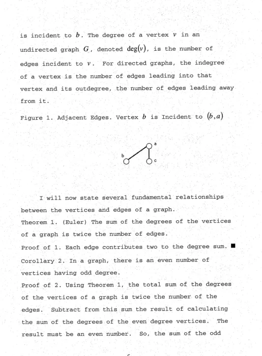
is incident to &. The degree of a vertex V in an

undirected graph G , denoted deg(v), is the number of

edges incident to V. For directed graphs, the indegree

of a vertex is the number of edges leading into that

vertex and its outdegree, the number of edges leading away

from it

Figure 1. Adjacent Edges. Vertex b is Incident to {b,a)

I will how state several fundamental relationships

between the vertices and edges of a graph.

Theorem 1. (Euler) The sum of the degrees of the vertices

of a graph is twice the number of edges.

Proof of 1. Each edge contributes two to the degree sum, ■

Corollary 2. In a graph, there is an even number of

vertices having odd degree.

Proof of 2. Using Theorem 1, the total sum of the degrees of the vertices of a graph is twice the number of the

edges. Subtract from this sum the result of calculating

the sum of the degrees of the even degree vertices. The

degrees must also be even. Hence, there must be an even

number of vertices of odd degree. H

In a graph, a walk from vertex to vertex in­

, is a sequence W = ot ;vQTti.ces. A

trail is a walk with no repeated edges. A path is a trail

with no repeated vertices, with the possiblq exception of

the initial and final vertices, in which case then the

path is called closed. A closed path is called a cycle.

Paths can be indicated as sequences of adjacent vertices

such as, P =\a,b,C,

-■ • ,i, j

or by adjacent edges as in, the

notation P= ,b),(b ^c), - • ■ ,{h j),ij

• Vertdx i is

reachable from vertex _/' if there is a path from / to i .

A graph is connected if for every pair of vertices i and

j, there is a path from / to i.

Every path can be compared to other paths by its

length that can be in units of distance, time, money and

SO on. A collection of edge-weights, indicated as

will form a weighted graph that is a graph where

every edge is assigned a number. I will use the letter

"t" because the weights we consider will be the time it

takes to transverse an edge. The length of a path, P,

between two vertices on G is then given by

indicate the shortest distance between two vertices /, ye V of G.

A type of graph that contains no cycles but is still connected and contains the shortest distance between any

two vertices is a tree. It is well known that a tree with

n vertices, where neN a natural number, has exactly n—\ edges. [6] This leads to the existence of a unique path between any two vertices on the tree. A sub-tree of an undirected graph is a connected subgraph that has no

cycles. A spanning tree of a graph G is a subtree that

contains the complete set of vertices of G.

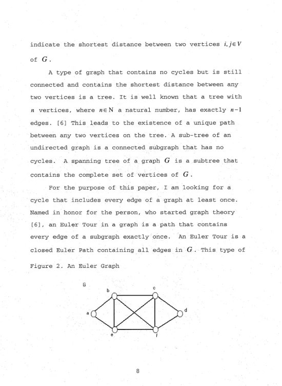
For the purpose of this paper, I am looking for a: cycle tha:t includes every edge of a graph at least once. Named in honor for the person, who started graph theory [6], an Euler Tour in a graph is a path that contains

eveJ-y edge of a subgraph exactly pnce. An Euler Tour is a

closed Euler Path containing all edges in G. This type of

tour is the focus of this paper for it allows our postman to start at one vertex, travel the edges of the graph and

end up at the starting vertex. An Euler Graph is a graph

that has an Euler Tour. Theses simple but useful

characterizations of both Euler Graphs and graphs with Euler Tours help form the following theorem.

Theorem 3. Euler's Theorem. A connected undirected graph

is an Euler Graph thus processes an Euler Tour if and only

if all vertices of the graph have even degree.

The proof of Theorem 3, although not difficult, is

somewhat lengthy and I have it available in APPENDIX ONE.

But, I will illustrate one direction of the procedure used

on the Euler Graph of Figure 2.

In Figure 2, consider the vertex b and we can form

an Euler eye1e identifled to be Pj =(p,C,d,f,

. In this

case, Pj is not an Euler Tour since it does not contain'

all edges and vertices of G/ However, /' is a vertex of

Pj that is incident with edges not on P,. We now begin a

trail P^ at /

that contains edges not belonging to Pj.

If we continue as long as we can, one possible choice

of P^ would be

-l^f,c,e,a,h,f). We now insert P^ into P,

at the first place / is encountered, obtaining

entire graph G. An Euler Tour is not unique; we just

ensure that every edge of G is use exactly once.

I now wish to state the Chinese Postman Problem.

Consider a mailman who is responsible for the delivery of

mail in an area of the city a^ in Figure 3. The mailman must always begin his delivery route at the same corner.

This will be a vertex on a graph. Figure 4. He then walks

every single street in his area; the edges of a graph; and, eventually, must return to the corner he started

from.

The most natural question to ask in this case is: How should the mailman's route be designed to minimize the total time he spends delivering the mail, while at the same time traversing every street segment at least once?

This type of edge-covering problem is known as the Figure 3. Picture of a City

■

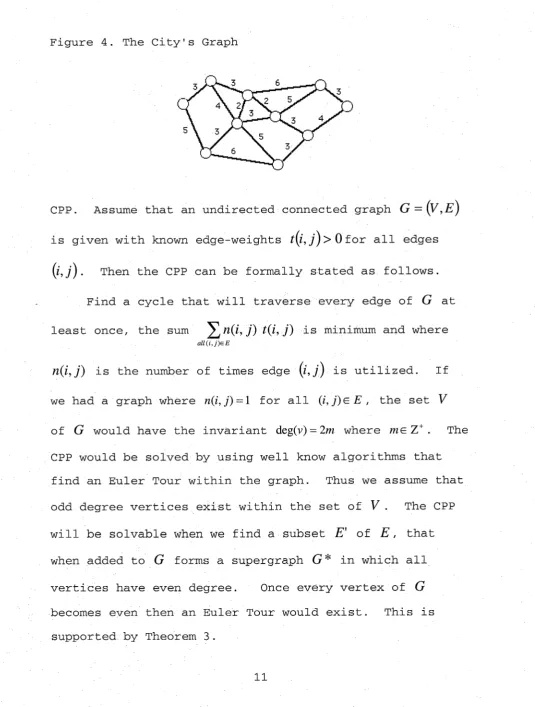
Figure 4. The City's Graph

CPP. Assume that an undirected connected graph G =(y,E^

is given with known edge-weights Ofor all edges

(1,7). Then the CPP can be formally stated as follows.

Find a cycle that will traverse every edge of G at

least once, the sum j) t(i,j) is minirnum and where

all{i,j)eE

n(i,j) is the number of times edge (z,/) is utilized. If

we had a graph where n(i,j)=l for all (i,j)eE, the set V

of G would have the invariant deg(v)= 2m where me Z"^ . The

CPP would be solved by using well know algorithms that find an Euler Tour within the graph. Thus we assume that

odd degree vertices exist within the set of V . The CPP

will be solvable when we find a subset E' of E, that

when added to G forms a supergraph G* in which all

vertices have even degree. Once every vertex of G

becomes even then an Euler Tour would exist. This is

supported by Theorem 3.

This result is exactly what the authors Tucker and

Bodin [3] did when they found a way to route the street

sweeping operations in the city of New York.

CHAPTER TWO

Tucker and Bodin [3] developed an efficient algorithm

to route street sweepers throughout the city of New York.

They had many obstacles to overcome among which were

parked cars, rush hour traffic and one-way streets. A

postman walking his route does not face these and many

other obstacles, but the algorithm in their paper will

still be very useful. The most noticeable change from the street sweepers to a postman problem is not using a

directed graph. instead, our postman uses an undirected

graph, because one way streets do not hamper him.

I will list the steps of, the algorithm from Tucker

and Bodin paper that I will integrate and provide a

detailed description with examples.

Let's start with a connected undirected graph

G=(V,E) and find the set V of odd degree vertices of G

(note that Vc F). The constructipn of this set is done

by inspection.

We will need the find shortest distance between any

pair of odd degree vertices Using a shortest path

algorithm to find paths in G does this.

With the members of V identified and the shortest

distance between any pair Of vertices in V also known,

one constructs the complete graph K of the vertices of

V' and with weights equaling d(i,j)3iJeV. The next step

is to find a minimal matching between the members of V .

A matching is a set of edges in K that have no endpoint

in common. A minimal matching is a pa.ir of vertices from

V and its edge weight such that no other pair has a

lower edge weight. This set will identify which paths,

when totaled together, will result in the minimum number

of edges and their weights to add to G.

Each path iP is known by a sequence of edges. For

each edge (x,y) on P, we add to graph G a duplicate copy

of edge (x,y) with weight /(x,y). Note that ^t(x,y)=d(i,j).

(x,y)eP

I will add the edges of every path found in the matching

phase to G. We have formed G* a supergraph of G .

At this point all vertices of G* are of even degree

and G* is called an Euler graph. There are several

well-known algorithms to construct an Euler Tour C in G*

which will become the optimal postman tour of the original

G. Once this algorithm is finished, the Chinese Postman

Problem is solved.

Let's look at each step in more detail and start by

finding V, a set of odd degree vertices. Since I am

starting with a connected undirected graph, G-(V,E), I

will assume that some number of vertices have odd degrees.

Othejrwis©, an Eul©]r Tour alraady exists and. the solution

can be found immediately. Recall Corollary 2 which states

that cardinality of V will be of the form Ik where k

will be later shown to be the number of paths added to G.

Here is an example to show how to find V . Let G

be a graph.

Figure 5. A Graph with Odd and Even Vertices

Table 1. Cardinality Information of Figure 5

~ c,d^ }

Vc={b,c,d,e}

CardiV(j')=4

As you can see in G , if an edge was added to G,

then the Carcl(V')=6. If an edge (h,f^ was added to G

instea:d, will not be an element of 1^', but / will be

an element of V and the CardiV')=4.

With the members of G identified, the shortest path

algorithm [6] is used to record the shortest path in G

between any i,jGV'. For very large n=Ccird(y'}, this step f

xs very time consuming. In fact, it would take ———

iterations to find the shortest paths between the vertices

of V. Loops, which are edges with the same vertex on

its endpoints, will be avoided.

Start with any isV and ask the question 'Are there

any vertices of G within one unit of i? If there is one

or more, say je V , label that vertex The label is not unique because there maybe other vertices one unit

from our starting vertex. The, ordered pair will let us

know that j or any other vertex is one unit from i . If

there are members of V not labeled with an order pair,

continue by asking the same question but increase the

distance by one. Repeat this for vertex j until all

elements of V have been labeled. Once i is used to find

a path with every other member of V, i is not considered

in further iterations of the algorithm. The process

starts again for a remaining member of V . Vertex i

isn't considered because there is no difference between

d{i,j) and d{j,i).

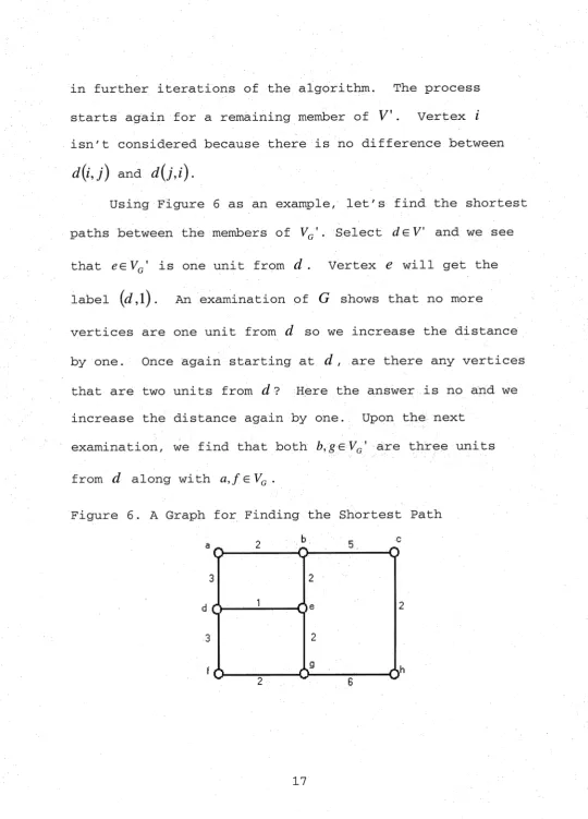
Using Figure 6 as an example, let's find the shortest

paths between the members of V^'. Select dGV and we see

that eeVg' is one unit from d . Vertex e will get the

label An examination of G shows that no more vertices are one unit from d so we increase the distance

by one. Once again starting at d , are there any vertices

that are two units from d? Here the answer is no and we increase the distance again by one. Upon theinext

examination, we find that both are three units

from d along with a,feVQ.

Figure 6. A Graph for Finding the Shbrtest Path

o o o

dO o

o o o

Table 2. Elements of V;, and from Figure 6

Vq ={a,b,c,d,e,f,g,h}

Vc'={b,d,e,g}

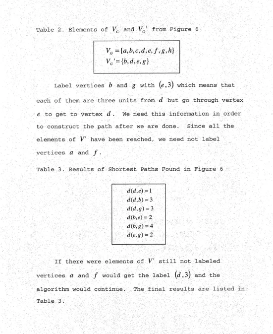
; Label vertices & and g: witb {e,3) which -means that

each Of them are three uhits frdm b? but go through vertex

e to get to vertex d . We need this information in order

to construct the path after we are done. Since all the elements of V have been reached, we need not label

vertices a and JP . ;

Table 3. Results of Shortest Paths Found in Figure 6

d{,d,e)=\ d{d,b)= 3 d{d,g)^3 d{b,e)= 2 d(b,g)= 4 d(e,g)= 2

If there were elements of V still not labeled

vertices a and f would get the label (d,3^ and the

algorithm would continue. The final results are listed in

Table 3.

Let be a coirt^^ graph where n>=Cflrrf(V^') as seen

in Figure 7. With the elements of V and all the

shortest paths found, I want to select pairs of vertices

of V' such that a maximal matching occurs. A maximal

matching in K„ is a set of edges that have no endpoint in

common and all n vertices are used. The result of

finding this matching will produce the minimum sum of the

edge weights. In Figure 7 we that edges {b,C^ and (d,

form the maximal matching.

Figure 7. Matching Odd Vertices

0

Let AT,,, be a complete graph such that

=(V,E) and

V^'cV where V is the set of odd vertices. Also, let the

set V be itemized such that the members of V are

individually assigned to the set {l,2,3v'? Card V"}. The

minimization of the sum of edges problem involving the maximal matching of vertices can be expressed in the following terms.

Let x^j, corresponding to edge {i,]), equal one if it

is a matching edge or zero if it is a non-matching edge.

The variable t(i,j) will be the weight of the edge. Then

the objective is to minimize:

Z = Min ^t(i,j)x.j

(1)

l<i<j<n

such that for each vE.V^

v-l

i:

i=\ y=v+i

Equations 1 and 2 are called constraints.

The algorithm that I will use to minimize Z in

equation 1 comes from a part of Operations Research called

Enumerative Techniques.[7] Enumerative Techniques simply

generates a list of possible solutions, finds the value of

each one and chooses the best. I will use a sequential

technique called the Zero-One Method of Balas. Balas used

a bound and branch enumeration that is a sequential

technique for solving combinatorial optimization problems and will greatly reduce the number of possibilities I need

to consider.

Possible solutions will fall into two areas, feasible or infeasible. Given the constraint X>1, a feasible solution is X — 8 because the statement is true for that value. An infeasible solution is X =0.

in Balas'method, if a solution is infeasible, an upper bound, or the closest possible integer solution, is : calculated and two new solutions are generated from the bounding routine. Solutions can be eliminated altogether

if it can be shown that a constraint can't ever be

satisfied. For example, if the variables a, b, C can only

equal one or zero, then for a constraint Cl + h + C = 7. where

a = h =0, this is an impossible solution and would be eliminated. These routines continue until finally the optimal solution is reached or no solution is possible.

This algorithm incorporates all the enumeration techniques needed to solve my matching problem because either an edge gets used (assigned a one) or not (assigned a zero). Balas also uses a decision tree to keep track of

the iterations. The next iteration is decided by the

largest upper bound. The conditions of my minimization problem described earlier are not set up to use Balas' method because he developed a maximization algorithm. However, a simple substitution in my description of the matching problem will result in an equivalent maximization

problem. I will start by substituting x.j'=l-Xij. This

equation still supports x.j' as an element of {0,1} since

if.Xjj = 1 then and vise versa. ; My problem is now

equivalent to:

Z'= Max (3)

l<i<jSn

such that for each vgV and n = CcirdV'

v-l

i=l j=v+l

where

x,'g{0,1}

0 matching

1 non-matching

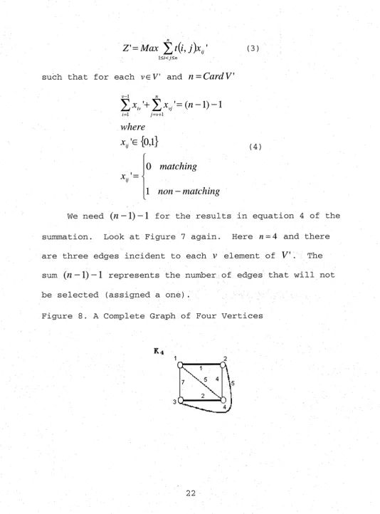
We need («— 1)— 1 for the results in equation 4 of the

suinmation. Look at Figure 7 again. Here n-A and there

are three edges incident to each V element of V . : The

sum (« —1)—1 represents the number of edges that will not

be selected (assigned a one).

Figure 8. A Complete Graph of Four Vertices

K.

The steps of the Balas method are best shown through

an example. Let be a complete graph as in Figure 8.

I will maximize

Z'= Xi2'+7Xi3'+5Xi4'+5^23'+4:\:24'+2X3/

. (5)

such that

X12'+X13'+Xi4'= 2

(6)

•^12'+^23'+-^24'= 2 (7)

^13'+^23'+^34'= 2 :

(8)

Xi4'+X24'+X34'=2

(.9)

We will begin by establishing three sets to track our

variable x,.,.' throughout the algorithm. We have:

W : The set of variables assigned a value of one. V : The set of variables assigned a value of zero. F : The set of unassigned variables.

Initially all are assigned to set F , point (1)

in Figure 9, and W and V both equal the null set. Then

for all .v.;' in F , let .v„.

U' assume the temporary value of IJ

one. Check the constraints, equations 6 through 9, with

all .V* '= 1, to see if we found a feasible, an infeasible,

or an impossible solution. If the solution satisfies the

constraints, then we have a feasible solution. If the solution is infeasible, as in our case with the

information in point (1), an upper bound, UB, on the value

of the optimal solution can be found. This bound is equal

to

UB= ^t(ij)+^t{i,j)-iocd^

(10)

Xjj'GW Xij'eF

An impossible solution exists if one of the

constraints was

+

and

^23 ^ •

Although

infeasible, this situation is also impossible because No bounding and branching would take place and

the point that contained this- information would be

eliminated from further consideration.

So, our first bound, using point (1) and equation 10

will be 23=0+24 — 1. The minimum t(i,

came from ^52'.

When a solution is found to be infeasible but still

possible, its point in the decision tree sprouts two new

points labeled points (2) and (3) in Figure 9. This is

the branching step.

The set F is now the quotient FI in points (2)

and (3). Within point (2), is an element of W . The

set V is still the null set. Within point (3), x^^' is an

element of V . The set W is still the null set.

Feasibility is tested at point (2) to see if 23 will

be the optimal solution. Temporarily assign the value of

Figure 9./Bound and Branch of Point 1

UB=23

All X F

(Point 1)

eW

(Point 2) (Points)

one to all X.j' in F. We already have .t,,'=1 because A'l^'

is an element of W . This is the same situation that we were in at point (1), thus infeasible. Bound point (2) with the value of 22 using equation 10 and shown in Figure 10. Next, branch two new points (4) and (5) using

because the min t\i, J) in equation 10 came from X^^ .

With two UBs, one for point (1) and the other for (2), select the largest UB to continue the feasibility test. The largest UB applies to point (1) because 23 > 22

and directs us to test point (3). Since belongs to V

and '= 0, two of the constraints, equations 8 and 9, are not satisfied while the all other members of F are equal to one.

Figure 10. Bound and Branch of Point 2

UB=22

(Point 2)

x ',x 'eW

(Point 5)

(Point 4)

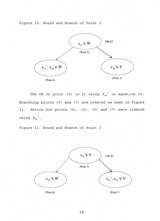
The UB on point (3) is 21 using ^34' in equation 10.

Branching points (6) and (7) are created as seen in Figure 11. Notice how points (4), (5), (5) and (7) were created using X_{34 •}

Figure 11,. Bound and Branch of Point 3

X 'g V UB=21

(Point 3)

X3,'GW _{•^12 9 -^34^^}

(Point 6) (Point 7)

Points (2) and (3) to UBs / ; We always seleGt.

the point with the largest UB in order to decide which,

point to next test. Since the bound of point (2) is 22,

point (4) and (5) are cohsidered for testing. The

information obtained from Point (4) doesn't change our

situation. All will equal one so we have

unfeasibility. The upper bound for point (4) is 20 since

20=3+21 — 4 and ^24' represents the minimum t{i, y). We

branch two new points (8) and (9).

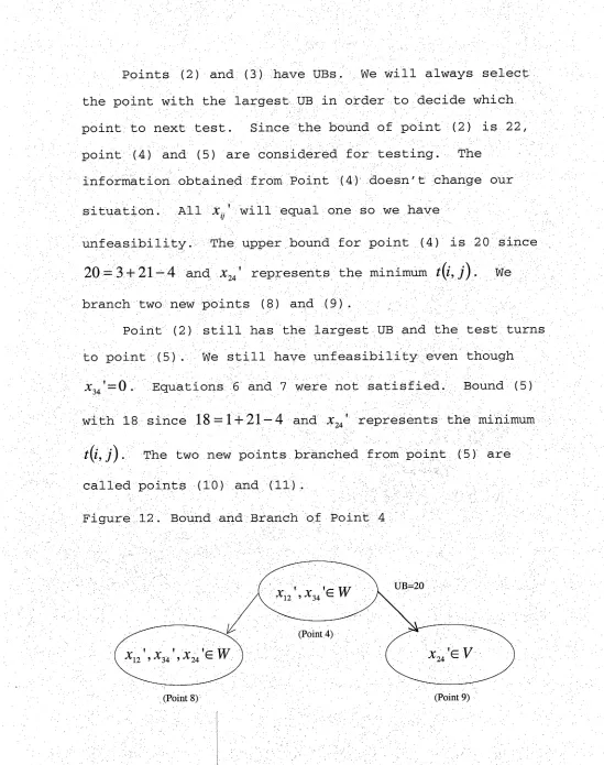
Point (2) still has the largest UB and the test turns to point (5). We still have unfeasibility even though

^34'=0. Equations 6 and 7 were not satisfied. Bound (5)

with 18 since 18 = 1+21 — 4 and X24' represents the minim-um

t\i,j). The two new points branched from point (5) are

called points (10) and (11).

Figure 12. Bound and Branch of Point 4 ,■

UB=20

^12 ' -^34 ^ "

(Point 4)

w _{^24 ey}

: (Point 8) (Point 9)

Figure 13. Bound and Branch of Point 5

UB=18 ^34 eV

(Point 5)

X X G y

Xi2, ,^34 G W ■^34 ' -^24 ^ '

(Point 10) _{(Point 11)}

The largest upper bound, found by looking at pbints

(3) , (4) , and (5) , is 21 given by point (3) . Upon examination of point (6) , it doesn't give a feasible

solution so its UB becomes 19 and points (12) and (13)

branch from (6) .

Figure 14. Bound and Branch of Point 6

UB=t9

(Point 6)

^3^ ,xJeW X ■ X _{■^12 -^24 ^ ^} G y

(Point 12) (Point 13)

Point {3)'s UB is still the largest so point (7) is checked for feasibility. We have a feasible solution with

point (7) because when X^2'=^34~^' equations 6 through

9 are now true statements.

Since the points (4), (5), and (6) upper bounds are

20, 18, and 19 respectively, they are eliminated because 21 from point (3) is the greatest upper bound to produce a

feasible solution. With = 0 =^34, this translates into

matching edges (1,2) and (3,4), as seen by the darken edges in Figure 8. The paths that produce the minimum weight when summed are now known.

We have shown that the paths with lengths

,y) can

be identified by the matching algorithm. The number of CardiV) 2k ,

paths we found will always be -= —:= This

2 2

conclusion is supported by Theorem 1 that showed each edge

contributes two to the Cardinality of V. Recall the

paths are connected collection of edges with no repeated vertices. We return to G and add each path in turn to

form the supergraph G*.

Select one of the ^ paths. Each path is a sequence

of edges starting with

and ending with (y*,7). For

each (x,3^)e P, add to G a duplicate copy of (x,y) and

also include /(x,y), the edge-weight. Once all the

have been added to G , we have a graph G* and will have

even degree vertices.

Let's further show what is happening with an example

Recall the graph from Figure 6. The edge weights and

results of the matching algorithm are:

Table 4. Matching Algorithm Results

d(d,e)=i

I\={(d,e)y

p^^{(b,e),(e,g)}

In Figure 15 we paved Path containing the edge

(d,e^ to G and start our creation of G*. Notice that

the deg(d) and deg(e)

In Figure 16 we pave the entire Pj which will make

and deg(g) even. You will also see that we also

kept deg(e) even.

With G* now a connected undirected graph where each

deg(v), VEVq^ is even, we know an Etiler Tour exists as

shown in Theorem 3.

Figure 15. Adding Path 1

G + P

I a 2

o o

o

d O Oe

3

o

Figure 16. Adding Path 2, Result is G

O o

le

dQ

o O

Taijle 5.'Graph G * Vertex Information

V '={a,b,c,d,e,f,g,h}

Recall that in the description of the CPP, we use

every edge of G* at least once. So, we will use every

edge of G once plus we will walk down the edges we added

from P^,x-l,...,k ,

Finding the Euler Tour is a well-known algorithm

requiring the type of graph G* turns out to be.[6] When

we first start, all the edges in G* are considered

unused. Imagine our mailman just showed up for work in

his neighborhood and has not started to deliver mail. His

neighborhood looks just like Figure 16. Generally, we may

start at any vertex in G* and begin to construct a

closed trail T in G*. Recall a closed trail is a walk

with no repeated edges. So a closed trail also starts and

stops with the same vertex.

While there are edges in G* that are not yet in

trail T", choose any vertex; i that is in T" incident with

an unused edge. The vertex it is a new starting point to

construct another closed trail D of unused edges in G*.

Once you reach vertex i at the end of the trail, splice

trail D onto T at vertex j. This process continues

until there are no more unused edges in G* and all edges

are now in Z". Using Figure 17, we begin at vertex Q, and

form the trail T ={{a,b),{b,e),{e,g),{g,f),{f,d),{d,a)}.

Figure 17. G* with Trail T Showii

G *

O

o

The colored in vertices helps show the trail T .

Select a vertex on T and an unused edge incident to it, like vertex d. We start the next trail between vertices

d and e . Then trail D will become

D ={{d,e),(e,g),(g,h),(Jt,c),{c,b),$b,e),(e,d)} in Figure 18

Figure 18. Graph G* with Trail D Shown

o

o

Splice trail D into T where edge {f,d) in T is

arranged. The resulting tour uses each edge of G* once

for a minimum tour length of 33 time units since T

becomes:

T -{{a,b),{b,e),{e,g),{g,/),(/,d),{d,e),(e,g),ig,h),(h,c),(c,b),(b,e),(e,d),(d,a)}

CHAPTER THREE ^

We just reed about an efficient set of algorithms

that found an optimal solution to the Chinese Postman

Problem. The main result of these algorithms was adding a

set of edges for a graph G. These edges, in the form of

paths, were found by obtaining a matching between odd

degree vertices. The sum of the path distances between

matched vertices was kept to a minimum. So, the addition

of these paths, or set of edges, to G produced an Euler

Graph and an optimal Euler Tour.

The process just discussed could be viewed as a

global approach to solving the CPP. Almost every step

considered the entire graph in one way or another. The

next algorithm 1 wish to discuss takes a local approach to

finding the optimal solution to the CPP. Instead of

finding paths by matching vertices, we will now grow the

paths one edge at a time.

We start with a graph containing odd degree vertices

as before as seen in Figure 19. When we grow the paths

one edge at a time, we are really looking for the edge

that will increase the total distance" traveled by the

mailman the least. The edge we add to the path is called

a matching edg's• As you may know, using this simple step

blindly will not always ensure an optimal solution.

Figure 19. Graph with Edge Weights

0

In Figure 19, the simple approach would add the edge

weights of 1, 5, and 6 in order to produce an Euler Graph. But, it is clearly evident that only the edge weight of 9 is needed../

A detailed algorithm written by Edmonds and Johnson [5] includes a clever way to adjust for poor choices one might make in such a simple /view of things. Unfortunately, this clever adjustment is very complex and beyond the

scope of this paper.

I will now give a general description of the Edmonds and Johnson algorithm for the optimal solution to the CPP. I will finish by illustrating it with an example.

We m.ust keep track of which edge to include at any given iteration, Edmonds and Johnson developed an ordered

triple

,/y^) to assign to each vertex and a revised

cost Cg to each edge. I will use instead of for uniformity. Each of the iterations of the algorithm will involve the assignment of a matching edge and/or the

forming of an object called a blossom until the end of the algorithm. Before the next iterati^o^ beginS/ an

adjustment of the ordered triple and the revised costs is necessary to identify the next matching edge or blossom to be created. Each of these assignments and adjustments will be explained.

The assignment of matching edges is a very desirable result because this can lead us to the path we are

growing. To describe when a matching edge is assigned we

must first describe the planted forest F that contains ■

the endpoints of the matching edge. Starting with

G =(y,E^ find V which consists of the odd degree

vertices of G .

Each vertex in V' is named a psuedovertex (PV) and

is considered a tree consisting of a single vertex. This

collection of trees forms the initial planted forest F .

Psuedovertices are also called outer or inner vertices. An outer vertex is deficient if it is not incident to a i

matching edge. Initially all PVs are outer vertices and

are deficient. An inner vertex is a member of a tree that

has one matching and one non-matching edge incident to it. Also, an inner vertex is incident to two outer vertices

For each of the iterations, every tree in F has one

deficient PV consisting of only one outer vertex or the

tree consists of a number of outer and inner vertices

incident along with matching and non-matching edges. In the Figure 20, a plus symbol on a vertex will identify an outer vertex and the minus symbol will idehtify an inner vertex. ;

Figure 20. Trees of the Forest F

□

Outer yertex Outer and inner vertices

as a tree as a tree

Matching edge —— non-matching edge

Now, the assignment of a matching edge happens when

the next shortest edge in G is an edge NOT in F

connecting two outer vertex trees in F . This

necessitates an augment and switch operation to ensure the alternating pattern of matching and non-matching edges

that exist between outer and inner vertices. No deficient

PVs exist after augment and switch, so the trees are

removed from F ,

If the algorithm does not direct the assignment of a matching edge, the result of the iteration will involve

the assignment of blossoms. Blossoms, B , temporarily

hide portions of the graph to better determine how the

algorithm will continue and find the next matching

Figure 21. Augmenting of Matching Edges and Switching

□ □

Before

[j ED^^ZZhdZI

+ +

After

edge. Basically the blossom surrounds the elements of the

graph. The blossom is shrunk to a PV and then the original

graph temporarily becomes the quotient graph • The PV

will store the information it contains until the time it

is expanded, or blossoms. At different Stages of the

algorithm, there are three types of blossoms that can be

found. They are pictured in Figure 22.

Figure 22. Types of Blossoms

A) B) C)

/

Figure 22A shows a blossom that is an odd cycle. If

the matching edge (2,3) is switched, with non—matching edge

(3,4) along- with (5,4) switching witli Xl,5), then every:^^^^^ /,

veitex of the blossom will meet exactly one matching^ edge.

In Figure 22B, the circle vertex is an original vertex of

graph^G that can have any number of matching edges

incident to it. When edge (1,3) is switched to a

non-matching edge, each PV is incident to one non-matching edge.

In Figure 22C the original vertex meets one non-matching

edge of the blossom and any number of matching edges. If

the PV inside the blossom is met by a matching edge, such

as PVl, then swap all the matching and non-matching edges

Before any iteration can end, the adjustment phase of

the algorithm must take place to help identify the next

matching edge or blossom to be created. There are two

items requiring adjustment; the ordered triple of each

vertex and the revised cost which is the edge weight

',m)' V edges (v,u)e E, the edge set of G .^

;

To describe why the ordered triple, {d^,d^.

and

are adjusted one needs an intuitive idea of what

each are. The term J,; is the distance to a deficient PV

in a tree that V is in. ■ This distance is from at most

one edge length away. Next, is the distance to a

deficient PV in a tree that V is not in and is one vertex

from. In Figure 23, d~ =1 . The final variable of the ordered triple, is a storage position for an edge cost

that was subtracted or added to t(y,uy. If t(y,uy

decreases, then 3^^ will increase the same amount and vice

versa.

Figure 23. Graph G to Determine

:0

During the formation of blossoms, the values of any of these variables may need to be altered since the

blossom will itself shrink into a PV. If vertex V is not

adjacent to a PV, then d~-0°. After the formation of a blossom and the shrinking to form a PV named p, the

vertex v may be adjacent to p . If this is the case,

then value will change. Checking to see if this happens is called 'scanning p'. There are other

adjustments that may need to be made at the end of each of the iterations of the algorithm. They are similar in

nature to the above explanation and will be shown in an

upcoming example.

; At each of the iterations of the algorithm, the

ordered triple is used to find the nearest vertex and edge

to the patbs Gpnstructed so far. Matching edges are

assigned and/or blossoms are formed or expanded as

necessary. Then all the vertex's variables and edge

weights are adjusted to reflect this change to the graph.

This process continues until there are no deficient PVs

remaining in the planted forest F . When this occurs, the

PVs are expanded into blossoms to determine which edges in

G will become matching edges. The matching edges will

augment G thus turning G * into an Euler Graph. Recall

that adding edges to G will result in a supergraph named

G*. Let's see this now in the following example.

Figure 24. (Left) Graph G for E&J Example Figure 25. (Right) Forest F for E&J Example

o O _O""

+

o dO o ®

0+

o o

Graph0 Forest f

We begin by letting G = , where G/ is called a

surfaee graph., and' assigning to each vertex of

G . At the start of the algorithm y^. — 0 Vv G V and

cll ='^ except if v is a deficient PV, then dl =0. For

the edge weights, initially let t(y,u)= V(v,u)E E.

To calculate d~, let

d~ = imri|?(v,H)':M w oMfer

Let (v,w) be the edge giving the minimum above. If

there is no such (v,m), then d~ =°° and ?(v, m)'=0. Let's

look at vertex a and b in Figure 24. The degree of a is

an even number so a is an original vertex; the degree of

b is an odd number so it is a PV. We can assign d^ = oo ,

d~ = 1 since t(^,b)'= I and b is a PV. Finally =0 and the

ordered triple for vertex a is complete. For vertex b,

we will discover different values. We generate d^ =0,

dl =3 since vertex e is the PV closest to b and y^ =0.

The rest of the vertices have their values in Table 6.

Every iteration will begin at Step (1) and, where upon examination of each vertex's ordered triple, a minimum value over all vertices of G is found. (When I refer

Table 6. The Initial Ordered Triple Values of Graph G

a. (~,1.0)

e.

(0,2,0)

b, (0,3)0)

f. (o=,3,0)

c.

('*',3.0)

g.

(0,2,0)

d. (0,2,0)

h.

(~.3.0)

to names of the Steps in this paper, Step (1) or Step

(1)(B), I am using the same notation contained in Edmonds

and Johnson paper.) When a tie for the minimum value is

obtained, decide arbitrarily. The minimum over all

vertices in G will come from one of the following three

•j

cases found in Table 7 and be denoted a :

Table 7. Definitions for Step 1 Cases

{cc):d^ for v not in any planted tree',

(/^):^(< +C) for V an outer vertex of a planted tree',

(7)-

for V an inner vertex of a planted tree.

Step (1) results in a tie for =1 for vertex a

(case oc) and vertices , e, and (case f). The case

Y did not generate any values because there are no inner

vertices in the forest F .

Let's arbitrarily chose vertex e and go to Step

(1)(B). Arbitrarily choose d to be the other vertex

incident to edge ,d) because

value was found using

either vertex d or g. Since d and e are in different

planted trees, we jump to Step (2).

Initially {e,d^ is a non-matching edge between two

outer vertices that are deficient. We augment G by ;:

switching (e,d) for a matching edge. Since this is the

first iteration, nothing more is done with augmenting.

Later we will see more details. Vertices d and 6 are no

longer deficient because there is a matching edge between

them and they lose the title outer vertex. Graph G and

Forest F change appearance as seen in Figure 25 and 26.

You will see the forest grow trees and lose them at the

end of most iterations.

Now every vertex in G, is examined by looking at the

triple in Table 6. When we have triples where both d^>d

and

^d* we leave v,, as it is. Recall that d =1 so

vertices a , C , g , b will not have their v,, value

changed. When we have triples where d^ <d we replace .v,,

Figure 26. (Left) Graph G After 1st Iteration Figure 27. (Right) Forest F After 1st Iteration

o o O""

o®

o'

o o

Graph Forest F

by

+{d* -d^) and subtract d* —dl from

for every ;

edge incident to vertex V . Vertices b, d , e , g , will

have y,. =1 and you can see that y,, will store information

subtracted from t{v,uy. Graph will have the following

edge weights seen in Figure 28. We do not have d~ <d* for

this iteration, so adjusting costs and coordinates in this

case is not discussed at this time,

An examination of F in Figure 27 shows we still have

deficient PVs so we adjust all such that

= minj + t(y,m)':u is an outer 'vertex

(V,«)[ «

Figure 28. Graph G After 1st Iteration

O

O

Graph

and let (v,u) be the edge given the above minimum. If no

such (v,m) exist, let d~

and ^(v,m)=0. The triple is

now updated in Table 4 and we return to Step (1).

Table 8. The Ordered Triple Values After First Iteration

e.

a.

(o°,0,0)

(0,0,1)

b.

(0,oo,l)

(-,2,0)

c.

(°o,2,0)

(o,°°,i)

d.

(0,oo,l)

(-,2,0)

We finished our first iteration and start again at

Step (1) by finding the d*. This time case a gives us

the choice of d* =0 using vertex a . . Case jS will produce

an c>o for vertices h and g , the outelr vertices of F.

Case Y is still void because we have !no inner vertices.

with d* =0 for vertex a, the algorithm takes us

directly to Step (1)(A) (2) . Vertex a is an original

vertex of G and vertex b is incident to a,. Recall that

vertex b is an outer vertex and a member of F .

A blossom B is formed surrounding a, b, and the

edge {ci,b) as seen in Figure 22C earlier. Replace

by

the quotient graph G^jB and shrink B to form a new PV

named p . '

Figure 29. Forming a Blossom in Graph G^

■'i-P' - v. 'x ■ '

Blossom B

-o

do aO

'6

Graph GJB i

Psuedovertex p will assume the 'properties of vertex

b in other words it becomes an outer vertex and

deficient. Psuedovertex p will also; be a member of F as

seen in Figure 30.

Figure 30. Forest F with Psuedovertex p

P O""

0+

Forest F

The ordered triple for PV p will have the value

= d

and =0. The value of d~ will be determined at the

start of Step (1). For each edge in G, (whether in GjB

or not) meeting vertex Z?, subtract d* -d^ from t{b,uy and

adjust

by adding {d* -d*)+ y,^ . There are three edges

incident to b, but d —d^=Q so the weights of t{b,ay,

t(b,cy , and t(b,ey do not change this time.

Before this step in the algorithm can end and we

start at Step (1), we must scan p. Scanning p means to

look at every non-matching edge (v,p) of G, where V is

incident to p , and compare

to d^ +t(v,py . If

dp+t(v,py<d~ then let d'^+t(y,p)'-d^ . Recall, these

adjustments are necessary because forming a PV from a

blossom may move a vertex closer to a deficient PV thereby

lessening d~. Vertices C, d , and e are incident to p .

We have =0 for each calculation and the following

information from GJB and Table 4.

Table 9. Results of Scanning PV p

dl +t(c,py<d~

►0 + 2<2; d~ =2 (no change)

dl+t(d,py<d-

►0+0<oo; d-=0 = dl

d* +t(e,py<d~

►0 +l<0 ; d~ =0 (no change)

Thus, d^ will change because 0+ 0<oo is a true

statement. Coordinates d^ and d^ will not change because

0 + 2<2 and 0 + l<0 are both false statements. In other

words, forming a vertex like p made vertex d closer to a

deficient PV. The above calculations will update the

ordered triples in Table 6 and produce Table 10. Use

equation 12 to fill in the value of d^ and move back to

Step (1) .

^ Table 10 grew with the addition of p , but vertices

a and b will not be considered in the next iteration

because they are temporarily hidden inside the

psuedovertex p . 'i:

Table 10. Ordered Triple After^^S Iteration

H,Q,

(^,2,

(0,^,1)

(0,^,1)

h.

(^,2,

(0,^,0)

e.

Once again Step (1) will produce d*= 0 but this time

from vertices d or e and for case (X . Case P produced

infinity and case f void. We enter Step (1) (A) (1)

because this time the vertices under consideration began

this process as PVs. Let vertex d become the vertex that

caused d =0. This part of the algorithm will rename our

PVs and reassign them back to F . Vertex d will become

an inner vertex and is adjoined to vertex p , the matching

edge {d,e), and with vertex e . Vertex e will become an

outer vertex and d* wi11 equal d*. We scan e by looking

at the two non-matching edges {jp,e) and (g ,e). We have :

=0 for each calculation the scanning results in Table

11.1 V'

Table 11. Scanning Vertex e

dl+t{p,ey<d]

dy +t{g,ey< d'

So for {p-,e) we have 0+1<<^ and for {g,e) we have

0-f0<oo which both are true statements. Thus we change

and dg both to zero. The vertices will become a planted

tree in F such that contains two components as seen in

Figure 32. GJB doesn't change as seen in Figure 31.

Figure 31. (Left) Graph GJB After 3rd Iteration

Figure 32. (Right) Forest F After 3rd Iteration

b

-o _0""

d 0 3p® _{d o} +

0

0+

Graph JB Forest F

We finish up this iteration by using equation 12 and

adjusting our ordered triples. The results are recorded

in Table 12 and we start Step (1) again.

Table 12. Ordered Triple Results After the 3rd Iteration

a.

ko,o)

(°o,2,0)

b.

(0,oo,l)

(0,0,1)

c.

(~,2,0)

(oo,2,0)

d.

(0,0,1)

(0,0,0)

(0,0,1)

e.

Back to Step (1) where case a produces a two, case

jS produces a zero, and case y produces a one because

vertex d is an inner vertex. This is a first for case y ,

but case

produces d* =0 so we jump to Step (1)(B) of

the algorithm and then to Step (2) because vertices g and

e are in different planted trees.

When this happened during the first iteration we just

augmented with a matching edge. This time is

different because vertex e is part of a larger planted

tree that has its own matching edge {d,e^. Here the

augmenting path that will include (g,e) must alternate

matching and non-matching edges as we transverse the tree

to vertex p . Thus, (g,e) and (d,p) will be matching

edges where {d,e) will become a non-matching edge as seen

in Figure 33.

Figure 33. The Augment and Switch Phase of the 4th Iteration

b c

-o ■o

1

0® 2

0

Graph G^/B

At this time we have no more deficient vertices

because is an empty graph. We finish up Step (2) by

noting that for all VG G^/5 ,

>d and d^>d . Hence

the triples, of Table 12 and edge weights of GjB are

fixed. We now enter Step (3) for the first time.

In Step (3) , we are now ready to reveal an optimum

solution by identifying which of the edges in GjB will

become matching edges in G*, the supergraph. For edges

that are matching edges in GjB, let them remain matching

edges in G*. This applies to edges (a,<i) and (e,g).

We next expand the PVs of GjB to determine which

edges in the blossom should become a matching edge. There

is only one PV in this example that will become a blossom

and that is vertex p . This blossom is Of the type where

an original vertex meets one non-matching edge, {a,b\ and

any number of matching edges, to include the one we have

(a,d^. See Figure 22C.

Figure 33. The Euler Graph Resulting From E&J Algorithm

o o

o o

Graph G*

Since the original vertex is incident to a PV that is

deficient, i.e. no matching edge is incident to b, change

{a,b^ to a matching edge. The algorithm is complete as

seen in Figure 33. All vertices now have even degree; run the Euler tour algorithm as in CHAPTER TWO to get the

optimal tour.

7-^-v APPEaSFDIX ONB' .

;• Proof of Theorem 3.:■ ■

Suppose G is an Euler Graph. Then G contains an

Euler Tour T , which begins and ends at some vertex V . Since T contains all vertices of G , a path joins every

two vertices of G, so that G is connected. We now show

that every vertex of G is even.

First we consider a vertex u different from V . Since U is neither the first nor the last vertex of T,

each time U is encountered it is entered via some edge and exited via another edge; hence, each occurrence of ll in T increases the degree of u by two. Thus, u has even

In the case of the vertex v, each occurrence of V

except the first and the last contributes two to its degree, while the initial and final occurrences of V in

T contribute one each to the degree of V . Therefore,

every vertex of G has even degree.

We now consider the converse statement. Assume that

G is a connected undirected graph and every vertex in G

is even. We show that G is an Euler graph. Select a

vertex V of G, and begin a path P at V . We continue

this path as long as possible until we reach a vertex W

such that the only edges incident with W already belong

to P; hence, P cannot be continued, and we must stop. We claim that W = V. To establish this, suppose that W

did not equal V. On each occasion that is encountered

prior to the last time, we use one edge to enter W and

another edge to exit from W .

When W is encountered for the final time on P, only

one edge is used to enter W. Hence, an odd number of

edges incident with W appears on P . However, since W

has even degree, there must be at least one edge incident

with W that does not belong to P .

This implies that P can be continued and therefore

cannot terminate at w, if W did not equal V . We

conclude that w = V, and P is actually a circuit. If the

circuit P contains all the edges of G, then P is an

Euler Tour of G and G is an Euler Graph.

Suppose the circuit P does not contain all the edges

of G. Since G is connected, there must be at least one

vertex u on P that is incident with edges on P . Remove

the edges of P from G and consider the resulting

undirected graph H... - Sinee P does not contain all the

edges of G , the undirected graph H has edges.

Furthermore, every vertex belonging to P is incident

with an even number of edges of P; hence, every vertex in

H has even degree. Let H^ be the component of H

containing the vertex M . If we begin a path P^ in //j at

U and continue this trail as long as possible, then, as

before, Pj must end at u and Pj is a path. Now it is

possible to form a path of G , Beginning and ending at

V , which has more edges than P . we do this by taking

the path P and inserting the path Pj at a place where u

occurs.

If Cj contains all the edges of G , then Cj is an

Euler Tour and G is an Euler Graph. If C, does not

contain all the edges of G , then we may Continue the

above procedure until we finally obtain an Euler Tour of G because there are a finite amount of edges. ■

' REFERENCES :

[1] Guari, M. "Graphic Prograrnxning Using Odd or Even Points." Chinese Math 1 (1962): 273-277. [2] Newman, J. "Leonhard Euler and the Konigsberg

Bridges." Scientific American 189 (1953): 37-70

[3] Tucker, A. C, and Bodin, L. D. "A Model for Municipal

Street Swaopina Operations." Networks. 4 (1974) ;

/■ 65-94 .' ■ ■ ■ \ .

[4] Behzad M. Introduction to the Theory of Graphs.

Boston: Allyn and Bacon Inc, 1971

[5] Edmdndh J. and Johnson E.L. , "Matching, Euler Tours

and the Chinese Postman." Math Programming 5

;/(1973),:;.S^8-j24.' '- :i­

[6] Gross J. arid Yellen J. . Graph Theory and its

Applications. New York: CRC Press, 1999

[7] Foulds, L. R. . Optimization Technidues, An

Introduction, New York: Springer-Verlag, 1981