University of Pennsylvania
ScholarlyCommons
Publicly Accessible Penn Dissertations
2018
Essays In Empirical Asset Pricing
Irina Pimenova
University of Pennsylvania, irina.v.pimenova@gmail.com
Follow this and additional works at:
https://repository.upenn.edu/edissertations
Part of the
Economics Commons, and the
Finance and Financial Management Commons
This paper is posted at ScholarlyCommons.https://repository.upenn.edu/edissertations/2750 For more information, please contactrepository@pobox.upenn.edu.
Recommended Citation
Pimenova, Irina, "Essays In Empirical Asset Pricing" (2018).Publicly Accessible Penn Dissertations. 2750.
Essays In Empirical Asset Pricing
Abstract
In this dissertation, I revisit two problems in empirical asset pricing.
In Chapter 1, I propose a methodology to evaluate the validity of linear asset pricing factor models under short sale restrictions using a regression-based test.
The test is based on the revised null hypothesis that intercepts obtained from regressing excess returns of test assets on factor returns, usually referred to as alphas, are non-positive.
I show that under short sale restrictions a much larger set of models is supported by the data than without restrictions.
In particular, the Fama-French five-factor model augmented with the momentum factor is rejected less often than other models.
In Chapter 2, I investigate patterns of equity premium predictability in international capital markets and explore the robustness of common predictive variables.
In particular, I focus on predictive regressions with multiple predictors: dividend-price ratio, four interest rate variables, and inflation.
To obtain precise estimates, two estimation methods are employed.
First, I consider all capital markets jointly as a system of regressions.
Second, I take into account uncertainty about which potential predictors forecast excess returns by employing spike-and-slab prior.
My results suggest evidence in favor of predictability is weak both in- and out-of-sample and limited to a few countries.
The strong predictability observed on the U.S. market is rather exceptional.
In addition, my analysis shows that considering model uncertainty is essential as it leads to a statistically significant increase of investors’ welfare both in- and out-of-sample.
On the other hand, the welfare increase associated with considering capital markets jointly is relatively modest.
However, it leads to reconsider the relative importance of predictive variables because the variables that are statistically significant predictors in the country-specific regressions are insignificant when the capital markets are studied jointly.
In particular, my results suggest that the in-sample evidence in favor of the interest rate variables, that are believed to be among the most robust predictors by the literature, is spurious and is mostly driven by ignoring the cross-country information.
Degree Type
Dissertation
Degree Name
Doctor of Philosophy (PhD)
Graduate Group
Economics
First Advisor
Francis J. DiTraglia
Keywords
empirical asset pricing, return predictability, short sale constraint
Subject Categories
ESSAYS IN EMPIRICAL ASSET PRICING
Irina Pimenova
A DISSERTATION
in
Economics
Presented to the Faculties of the University of Pennsylvania
in
Partial Fulfillment of the Requirements for the
Degree of Doctor of Philosophy
2018
Supervisor of Dissertation
Francis J. DiTraglia, Assistant Professor of Economics
Graduate Group Chairperson
Jes´us Fern´andez-Villaverde, Professor of Economics
Dissertation Committee
Francis J. DiTraglia, Assistant Professor of Economics
Frank Schorfheide, Professor of Economics
ESSAYS IN EMPIRICAL ASSET PRICING
c
COPYRIGHT
2018
Irina Pimenova
This work is licensed under the
Creative Commons Attribution
NonCommercial-ShareAlike 4.0
International License (CC BY-NC-SA 4.0)
To view a copy of this license, visit
ACKNOWLEDGEMENT
The five years of graduate school have been a period of intense learning for me, not only
in the scientific arena, but also on a personal level. I would not have finished the graduate
school without the amazing people I have been surrounded by.
First and foremost I would like to thank my advisor, Professor Francis DiTraglia, for his
fundamental role in my doctoral work. I greatly appreciate his patient guidance,
encour-agement, and advice he has provided throughout my time as his student to make my Ph.D.
experience productive and stimulating.
I am also grateful to my other dissertation committee members, Professors Xu Cheng and
Frank Schorfheide, for their guidance and insightful comments. Without their help, this
dissertation could not be completed.
I am greatly indebted to Professor Jakub Jurek, who introduced me to the exciting world
of empirical finance and taught me how good applied research is done. I have learned a lot
from him, and the summers that I have spent working with him have been the highlights
of my graduate school experience.
I would like to thank my friends in the economics department for all the great times that
we have shared. I am particularly grateful to Hanna Wang for her infinite patience and
support.
Lastly, I would like to thank my family. I am grateful to my parents for all their love and
encouragement and for being there for me since day one. I thank my sister for being my
role model despite being younger than me. Without them, this thesis would never have
ABSTRACT
ESSAYS IN EMPIRICAL ASSET PRICING
Irina Pimenova
Francis J. DiTraglia
In this dissertation, I revisit two problems in empirical asset pricing. In Chapter 1, I propose
a methodology to evaluate the validity of linear asset pricing factor models under short sale
restrictions using a regression-based test. The test is based on the revised null hypothesis
that intercepts obtained from regressing excess returns of test assets on factor returns,
usu-ally referred to as alphas, are non-positive. I show that under short sale restrictions a much
larger set of models is supported by the data than without restrictions. In particular, the
Fama-French five-factor model augmented with the momentum factor is rejected less often
than other models. In Chapter 2, I investigate patterns of equity premium predictability
in international capital markets and explore the robustness of common predictive variables.
In particular, I focus on predictive regressions with multiple predictors: dividend-price
ra-tio, four interest rate variables, and inflation. To obtain precise estimates, two estimation
methods are employed. First, I consider all capital markets jointly as a system of
regres-sions. Second, I take into account uncertainty about which potential predictors forecast
excess returns by employing spike-and-slab prior. My results suggest evidence in favor of
predictability is weak both in- and out-of-sample and limited to a few countries. The strong
predictability observed on the U.S. market is rather exceptional. In addition, my analysis
shows that considering model uncertainty is essential as it leads to a statistically significant
increase of investors’ welfare both in- and out-of-sample. On the other hand, the welfare
increase associated with considering capital markets jointly is relatively modest. However,
it leads to reconsider the relative importance of predictive variables because the variables
that are statistically significant predictors in the country-specific regressions are
in-sample evidence in favor of the interest rate variables, that are believed to be among the
most robust predictors by the literature, is spurious and is mostly driven by ignoring the
cross-country information. Conversely, the dividend-price ratio emerges as the only robust
TABLE OF CONTENTS
ACKNOWLEDGEMENT . . . iii
ABSTRACT . . . iv
LIST OF TABLES . . . ix
LIST OF ILLUSTRATIONS . . . x
CHAPTER 1 : Short Alpha: Linear Factor Model Diagnostics Under Short Sale Constraints . . . 1
1.1 Introduction . . . 1
1.2 Econometric Methods . . . 4
1.3 Simulation: Comparing Finite-Sample Performance . . . 14
1.4 Application: Can Short Sale Restrictions Help to Explain Returns? . . . 18
1.5 Robustness Check: Transaction Costs . . . 25
1.6 Conclusion . . . 27
1.7 Appendix . . . 29
CHAPTER 2 : International Return Predictability . . . 31
2.1 Introduction . . . 31
2.2 Methodological Framework . . . 37
2.3 Data Overview . . . 43
2.4 In-Sample Analysis . . . 48
2.5 Out-of-sample Analysis . . . 61
2.6 Extensions . . . 68
2.8 Appendix . . . 87
LIST OF TABLES
TABLE 1 : Simulation Results for Mean Test . . . 17
TABLE 2 : Results for Sorts Based on Factors . . . 21
TABLE 3 : Results for Sorts Based on Anomalies . . . 23
TABLE 4 : Results for Industry Portfolios . . . 25
TABLE 5 : Required Transaction Costs . . . 26
TABLE 6 : Simulation for Mean Test with GARCH Disturbances . . . 29
TABLE 7 : Summary Statistics of International Returns . . . 46
TABLE 8 : Summary Statistics of Predictive Variables . . . 47
TABLE 9 : Models with Highest Posterior Odds . . . 50
TABLE 10 : Bayesian Estimates of Slope Parameters (Basic Specification). . . . 53
TABLE 11 : Bayesian Estimates of Inclusion Probabilities (Basic Specification) 54 TABLE 12 : In-Sample Asset Allocation . . . 59
TABLE 13 : In-Sample Certainty Equivalent Returns . . . 60
TABLE 14 : R2OOS (Basic Specification) . . . 63
TABLE 15 : Out-of-Sample Asset Allocation (Basic Specification) . . . 67
TABLE 16 : Out-of-Sample Certainty Equivalent Returns (Basic Specification) . 67 TABLE 17 : Bayesian Estimates of Inclusion Probabilities (Borrowing from Cross-Section) . . . 73
TABLE 18 : R2OOS (Borrowing From Cross-Section) . . . 76
TABLE 19 : Out-of-Sample Asset Allocation (Borrowing From Cross-Section) . 77 TABLE 20 : Out-of-Sample Certainty Equivalent Returns (Borrowing From Cross-Section) . . . 78
TABLE 21 : Bayesian Estimates of Inclusion Probabilities (Stochastic Volatility) 83 TABLE 22 : R2OOS (Stochastic Volatility) . . . 84
LIST OF ILLUSTRATIONS
FIGURE 1 : Illustration of Moment Selection . . . 7
FIGURE 2 : Posterior Distribution of Slope Coefficients (Basic Specification) . 49
FIGURE 3 : Net-SSE . . . 66
FIGURE 4 : Posterior Distribution of Slope Coefficients (Borrowing from
Cross-Section) . . . 72
CHAPTER 1 : Short Alpha: Linear Factor Model Diagnostics Under Short Sale
Constraints
1.1. Introduction
Standard econometric tests for evaluating the validity of a linear asset pricing factor model
with traded factors focus on intercepts, usually referred to as alphas, obtained from
regress-ing excess returns of test assets on factor returns.12 The alphas are expected to be jointly
zero if factors are mean-variance efficient, and the model is rejected if alphas are not zero.
However, these tests ignore a crucial assumption: mean-variance efficiency only implies zero
alphas in the absence of market frictions such as short sale restriction, taxes, transaction
costs, liquidity constraints, etc. The factor model may thus be rejected not because the
inspected factors are not mean-variance efficient, but rather due to the market frictions.
Very few papers re-consider the implications of mean-variance efficiency for factor model
testing in the presence of market frictions.
In this chapter I explore one of the most prominent market frictions: the short sale
restric-tion. A short sale is the sale of an asset that is not owned by the seller. This transaction
is risky as the potential loss is unlimited, expensive due to the lending fees, and in some
cases outright infeasible because of scarce lending markets. Consequently many investors
either can not or do not want to sell short and are thus short sale constrained. Short-sale
constraints are an important factor in determining asset prices as shown, for example, in
a survey by Rubinstein (2004).3 If short sales are constrained, negative alphas cannot be
arbitraged away. Hence, negative alphas are consistent with mean-variance efficiency under
a short sale restriction as shown by DeRoon and Nijman (2001) and AitSahlia et al. (2017).
1A recent survey of the econometrics underlying mean-variance efficiency tests can be found in Sentana
(2009).
2“Factor model” here is defined as a set of traded factors on the right hand side in the regression. The
model is considered to be valid if the factors are mean-variance efficient.
3There is large literature on the impact of short sale constraints on asset prices. The theoretical work
This leads me to propose a model validity test under the short sale constraint based on the
null hypothesis that alphas are non-positive.
The null hypothesis is an inequality restriction and is hence more difficult to test than an
equality-based null, so I employ the moment inequality literature, a strand of literature in
econometrics focusing on testing procedures exploring nulls that contain inequalities. In
particular, I apply two testing procedures: one suggested by Andrews and Soares (2010)
(AS) and one by Romano et al. (2014) (RSW). The difference between the two procedures
is explained later in the text. in addition to applying the methods, I compare their finite
sample properties in simulation, as this has not been done before. My findings suggest
that neither test exhibits size distortions in small samples and that both tests are robust
to conditional heteroscedasticity. I also find that the RSW is slightly less powerful that the
AS test.
Using these tests I evaluate several factor models (defined here as a combination of factors).
Among others, I examine the two classic models: the CAPM with a single market factor
proposed by Lintner (1965) and Sharpe (1964) and the Fama-French three factor model of
Fama and French (1993). I also include some more recent models such as theq-factor model
of Hou et al. (2014a) and the Fama-French five-factor model of Fama and French (2015b).
As the test assets I use sets of testing portfolios labeled as “pricing anomalies”.
I show that under short sale restrictions a much larger set of models is supported by the
data than without restrictions. In particular, the five factor model augmented with the
momentum factor is not rejected for multiple pricing anomalies when the short sale
re-strictions are taken into account. I also find some support for the four-factor model that
include the Fama-French three factors and the momentum factor. These findings suggest
that momentum factor is not redundant. In contrast, I strongly reject the CAPM and the
original Fama-French three-factor model and find limited support for theq-factor model for
almost all sets of test assets. These models are rejected even under the short sale restriction
One may hypothesize that the rejection is due to the transaction costs associated with
small portfolios. However, I show that the decision about which models are rejected or not
are robust after taking into account transaction costs. In particular, the CAPM and the
original Fama-French three-factor model require assuming very large transaction costs to
justify the mis-pricing.
This chapter contributes to the literature on mean-variance efficiency under short sale
re-striction. The literature on short sale restrictions in the context of factor models is limited
to the recent paper by Dugalic and Patino (2017), who build a CAPM-like structural model
with short sale constraints and obtain an equation that links asset-specific excess returns
with the market equity premium. However, the derived alphas are only valid if there is a
single risk factor, market factor, and extending this setup for other models is challenging
because it requires building a new structural model for each combination of factors. In
contrast, my approach can be easily applied to any set of traded factors.
This chapter is the first to consider mean-variance efficiency testing under short sale
restric-tions in the context of factor models, however, some papers studied it in different contexts.
In particular, DeRoon and Nijman (2001) and Li et al. (2003) test whether U.S. investors
can extend their efficient set by investing in emerging markets when accounting for short
sale restrictions. AitSahlia et al. (2017), Tang et al. (2010) and Elton et al. (2006) explore
the efficiency of portfolios offered in 401(k) plans under short sale restrictions. These papers
usually focus on one or two test assets, while testing the validity of factor models requires
using from ten to thirty test assets. Consequently, factor models testing requires tests that
have high power even if the number of test assets is large. For this reason, the testing
procedures I use differ from the ones used in earlier papers. I explain later in the chapter
how the two tests I consider maintain high power.
More generally, this chapter also contributes to the literature that compares asset pricing
factor models by testing them against pricing anomalies. The most recent study by Hou
-factor model of and the Fama-French five--factor model to be the best performing models.
As mentioned previously, this strand of literature does not take into account short sale
restrictions.
This chapter is organized as follows. In the second section, I present the econometric
frame-work and discuss the two testing procedures. Next I compare the finite sample performance
of the two types of tests in a simulation experiment. In the fourth section I apply the tests
to several linear factor models and multiple sets of test assets. Some concluding remarks
are offered in the final section.
1.2. Econometric Methods
This section presents the econometric framework, discusses the intuition behind inequality
testing and introduces two alternative procedures that can be used to test the null hypothesis
based on the papers by Andrews and Soares (2010) (AS) and Romano et al. (2014) (RSW).
1.2.1. Econometric Framework and Notation
Consider a linear asset pricing factor model:
Ri,t=αi+
K
X
k=1
βi,kfk,t+εi,t ∀i= 1, . . . , N, ∀t= 1, . . . T. (1.1)
The excess return over a risk free rate on an asset i, Ri,t (also called risk premium), is
linearly related toK traded risk factors,fk,t, with the sensitivity to a factorkgiven byβi,k
(beta). The alphaαi represents how much extra return an asset iis expected to deliver in
addition to the reward for risk represented by factors. The return in each period is affected
by an idiosyncratic shock εi,t. These shocks are jointly distributed with zero mean and a
nonsingular covariance matrix Σε.
For convenience, the model in (1.1) is re-written in matrix form. Stacking the returns for
K×1 vector βi yields:
Ri,t =αi+ft>βi+εi,t
Stacking returns on all assets in periodtinto aN×1 vectorRt, all idiosyncratic shocks at
periodtinto vector εt, and all factor loadingsβi into aN ×K matrixB yields:
Rt=α+Bft+εt, (1.2)
The model in (1.2) can be estimated by equation-by-equation OLS. OLS estimation in this
case is equivalent to estimating a system of unrelated equations because the right-hand-side
variables are the same for all test assets.
It is helpful to introduce some notation. The N ×1 estimated vector of alphas is denoted
b
α, and theN×N matrixΣbα is a consistent estimator of the covariance matrix of the scaled
vector of alphas,√Tαb. Theith diagonal element of the covariance matrix is denoted byσb2α,i.
I use bootstrap in the next section to construct the distribution of the test statistic under
the null. Let R denote the number of bootstrap samples generated for N assets observed
over T periods. For each bootstrap sample r, estimates of alphas αrb and the covariance
matrixΣbα,r are obtained. The significance level of the test is denoted bya.
1.2.2. Null Hypothesis and Test Statistic
The null hypothesis of factor mean-variance efficiency under short sale restriction is that
all alphas are non-positive:
H0:αi ≤0∀i= 1, . . . , N
H1:αi >0 for some i
(1.3)
The form of the null hypothesis in (1.3) was introduced by DeRoon and Nijman (2001),
verified by AitSahlia et al. (2017), who used direct portfolio optimization.
The intuition behind the null hypothesis in (1.3) is based on the idea of arbitrage. Assume
that the alpha αi is negative, so it delivers lower expected returns than other assets with
a similar risk profile. An arbitrage strategy to exploit this mis-pricing involves selling the
asset i short and buying a portfolio of factors. Consequently, if investors face short sale
restrictions for some assets and can not short sell the asset i, they cannot exploit the
arbitrage strategy, so the mis-pricing may persist with alpha remaining negative. Note also
that a combination of factors can be mean-variance efficient if the short sale restriction is
in place and not mean-variance efficient otherwise.
The test statistic for the null in (1.3) is motivated by the likelihood ratio test under the
assumption of normality but can also be applied if the assumption of normality does not
hold as in case of returns. This quasi-likelihood ratio (QLR), or Wald test statistic, first
introduced by Kudo (1963), takes the following form:
W =T inf
α0≤0 b
α−α0 >
b
Σ−α1 αb−α0
=T αb−αb(R−N)
> b
Σ−α1 αb−αb(R−N
(1.4)
where αb(R
−
N) is a restricted estimate of alpha under the non-positivity constraint. The
restriction on vector α0 ≤0 is to be understood component-wise. The Wald test statistic
in (1.4) can be seen as a weighted distance between the alphas, estimated with and without
the restriction of all elements being non-positive. Alphas that are originally “large” and
positive have more weight on the value of the test statistic because they are more likely to
be “far” from the corresponding non-positive estimator.
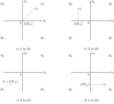
To develop the intuition behind the Wald statistic in (1.4), consider a simplified example
with two test assets. The covariance matrix of alphas is known and equal to an identity
matrix Σα = I. The identity covariance matrix yields two simplifications: 1. the Wald
test statistic is equal to a sum of squared deviations from zero and 2. under the diagonal
to the unrestricted estimate with positive elements set to zero (see Figure 1). In contrast,
under a non-diagonal covariance matrix, not only the positive elements are set to zero but
also the negative elements may take a new value.
b
α1 b
α2
0
Q1
Q2
Q3 Q4
b
α
b
α(R−N)
a)αb inQ1
b
α1 b
α2
0
Q1
Q2
Q3 Q4
b
α
b
α(R−N)
b) αb inQ2
b
α1 b
α2
0
Q1
Q2
Q3 Q4
b
α=αb(R−N)
c)αb inQ3
b
α1 b
α2
0
Q1
Q2
Q3 Q4
b
α
b
α(R−N)
d) αb inQ4
Figure 1: Illustration of Moment Selection
Four panels illustrate unrestricted estimates αb and restricted estimates under the
non-positivity constraintsαb(R−N) under the identity covariance matrix.
1. Note that the Wald test statistic in (1.4) and its asymptotic distribution is given by:
W =
0 ifαb∈Q1
b
α21∼χ21, ifαb∈Q2
b
α21+αb22 ∼χ22, ifαb1 ∈Q3
b
α22∼χ21, ifαb∈Q4
(1.5)
The distributional result in (1.5), which was obtained under identity covariance matrix, can
be generalized for any covariance matrix: given the number of non-negative elementsp, the
distribution of the test statistic is χ2 with p degrees of freedom. However, the number of
non-negative elements p is unknown. The unconditional distribution of the test statistic
in (1.4) under the null is then a mixture of χ2 distributions with weights given by the
probability that the estimated vector is in a given quadrant (conditional on the covariance
matrix). Kodde and Palm (1986) introduced a testing procedure based on this intuitively
appealing idea and showed that the test is asymptotically valid.
The Kodde and Palm (1986) test works great if the number of dimensions is small but shows
poor power properties if the dimensionality is large (which is the case for factor models).
As the number of non-negative elements p is actually unknown, the test is based on the
assumption that all inequalities can be binding. Suppose that the estimated alphas are in
the Q2 as in panel b in Figure 1 above with αb1 “far” from zero. The inequality αb1 ≤ 0
is not binding and does not influence the value of the test statistic. If the distribution
is constructed under the assumption that this inequality is potentially binding, it would
produce a high critical value.
The problem of low power is aggravated as dimensionality increases. With higher N this
test considers more and more areas which are not relevant for the case at hand, but do
influence the critical value. Suppose N −1 alphas are negative and ”far” from the zero
the value of the test statistic. If the critical value equally depends on negative and positive
alphas, it would be larger withN−1 negative alphas than it would be if the negative alphas
were absent. For bigN, the critical value would be especially large, leading to low power.
The solution to the low power problem in large N setting is to somehow isolate the
in-equalities that are “far” from binding, and treat them differently than potentially binding
inequalities - an approach called moment-selection.
1.2.3. Two Tests: AS and RSW
I consider two testing methodologies based on the idea of moment selection proposed by
Andrews and Soares (2010) and Romano et al. (2014). The two methods differ in how
they identify non-binding inequalities and use this information. Andrews and Soares (2010)
completely eliminate inequalities that are “far” from binding based on thet statistic when
constructing the distribution under the null. Romano et al. (2014) build a confidence
interval with a “small” significance level to identify inequalities that are “far” from binding,
and shift the null hypothesis, so that these constraints have a limited contribution to the
critical value. Other tests that implicitly or explicitly use the information were suggested by
Romano and Shaikh (2008), Andrews and Guggenberger (2009), Canay (2010) and Andrews
and Barwick (2012). The overview of the inequality-constrained inference can be found in
Silvapulle and Sen (2011).
AS Test
Andrews and Soares (2010) and Andrews and Barwick (2012) suggest to eliminate
inequal-ities that are “far” from binding when constructing the distribution of the test statistic in
(1.4) under the null. The suggested procedure consists of two steps: 1. determine
inequali-ties that are “far” from binding and 2. find the distribution of the test statistic using only
inequalities that are potentially binding.
context of this chapter the inequality is “far” from binding if the estimated alpha i is
negative and large relative to some cut-off parameter:
ti =− b
αi
b
σαi/
√
T > κ. (1.6)
A suitable choice ofκis based on Bayesian Information Criterion (BIC)κBIC = [ln(T)]1/2.4
The authors show in the simulation that this choice of the cut-off parameter results i a test
with good finite-sample properties.
The distribution is constructed via bootstrap after eliminating all alphas that satisfy the
inequality. After generating a bootstrap sample, all assets that satisfy the restriction are
eliminated from further consideration. The critical value is obtained as a 1−aquantile of
the bootstrapped distribution.
Algorithm for the AS testing procedure:
0. Estimate the linear factor model in (1.1) by OLS to obtain αb and Σ. Calculate theb
Wald test statistic in (1.4).
1. Find the “far” from binding inequalities.
(a) Calculate t-statistic for each alpha as in (1.6)
(b) Compare the value of the t-statistic with some cut-off value κ (e.g. κBIC) and
find the inequalities that are “far” from binding.
2. Estimate the distribution of the test statistic under the null and the corresponding
critical value at the significance level a.
4The performance of the procedure in finite samples is determined by the choice of the cut-off parameter
(a) Simulate R bootstrap samples each of sizeT.
(b) For each bootstrap sample r, estimate the linear factor model in (1.1) by OLS
to obtain αrb andΣbr.
(c) Eliminate the elements inαrb and Σbr that correspond to alphas that satisfy the
condition 1.6.
(d) Calculate the bootstrapped value of the Wald statistic as in (1.4), re-centered at
the estimated value of alphas in the original sample:
Wr=T inf
α0≤0 b
αr−αb−α0 >
b
Σ−α1 αrb −αb−α0
(e) Find the critical value as 1−aquantile.
RSW Test
Romano et al. (2014) suggested a two-step test. In the first step, a confidence region is
constructed at some “small” significance level b to determine which inequalities are “far”
from binding. This information is then used at the second step to estimate the distribution
of the test statistic. The procedure is designed to take into account that the actual value
of alpha may not be inside the confidence region, which is achieved by a Bonferonni-type
correction.
At the first step, an upper confidence rectangle for the vector of alphas is constructed at
the nominal level 1−bin order to determine which inequalities hold. The confidence region
is based on an inverted max t-statistic:
tmax= max
1≤i≤Nti = max1≤i≤N
αi−αbi
b
σ2
αi/
√
T (1.7)
observe at least this value is P r(tmax ≤d) = 1−b. The distribution of the maxt-statistic
is constructed via bootstrap, and the multiplier d is obtained as a 1−b quantile of the
distribution. The confidence region based on this bootstrap limits the possible values of the
true α. With probability at least 1−b the biggest possible value of the trueαi under the
null hypothesis is:
α∗i = min
b
αi+db σαi
√ T,0
(1.8)
Stacked together, they form a vector α∗.
In the second step, the confidence region obtained in step one is used to construct the
distribution of the Wald test statistic. The higher power is achieved by tightening the null
hypothesis. With probability at least 1−b, the value of the true population alphas under the
null is bounded above byα∗. Instead of computing the critical value for the least favorable
scenario under the nullα = 0, we can compute the critical value using the largest possible
value under the null α = α∗ ≤ 0. This is equivalent to shifting the null hypothesis from
α≤0 to α≤α∗. The Wald test statistic in (1.4) can be modified as follows:
f
W =T inf
α0≤α∗ b
α−α0 >
b
Σ−α1 αb−α0
=T inf
α∗
0≤0
b
α+α∗−α∗0> b
Σ−α1 αb+α∗−α∗0), (1.9)
whereα∗0=α0−α∗. We can now bootstrap the distribution of the Wald statistic.
This test is conservative by construction. It fails to reject the null in two cases: when either
test statistic is less than or equal to the critical value, or when all values in the confidence
region are negative. In order to account for the fact that alphas may actually be outside
of the confidence region with probability at most b, the null hypothesis should be rejected
if the value of the test statistic exceeds 1−a+bquantile of the bootstrapped distribution
rather than 1−aquantile.
0. Estimate the linear factor model in (1.1) by OLS to obtain αb and Σ. Calculate theb
Wald test statistic in (1.4).
1. Construct the 1−bconfidence region.
(a) Simulate R bootstrap samples each of sizeT.
(b) For each bootstrap sample r, estimate the linear factor model in (1.1) by OLS
to obtain αbr andΣbr.
(c) For each bootstrap sample r, calculate the bootstrapped value of the max t
-statistic as in (1.4) re-centered at the estimated value of alphas in the original
sample:
tmaxr = max
1≤i≤N
b
αi−αi,rb
b
σ2
αi,r/
√ T.
(d) Find the 1−b quantile of the maxt-statistic distribution d.
(e) Find the upper bound of the confidence region on the true alphas under the null
α∗ as in (1.8).
2. Estimate the distribution of the test statistic under the null and the corresponding
critical value at the significance level a.
(a) Bootstrap the data creatingR bootstrap samples.
(b) For each bootstrap sample r, calculate the bootstrapped value of the modified
Wald statistic under the tighter null hypothesis as in (1.9). The bootstrapped
statistic is re-centered at the estimated value of alphas in the original sample:
f
Wr=T inf
α∗0≤0 αrb −αb+α
∗−
α∗0>Σb−α1 αb−αb+α∗−α∗0
.
The properties of the testing procedure depend on the choice of the significance level b.
We can find an “optimal” value of b that maximizes the weighted average power. The
drawback of this approach is that finding the maximum is difficult and this can only be
done in simulation. The simulation results would only be valid for specific parametric
assumptions and under a specific vector of alternatives, for which the power is computed.
The authors found that a reasonable value of b is a/10. Larger values of b result in lower
power, while lower values of bdo not provide a noticeable increase in power but require a
larger number of bootstrap samples to accurately estimate the quantile.
1.3. Simulation: Comparing Finite-Sample Performance
This section compares finite-sample properties of the AS and the RSW tests. The simulation
focuses on a testing inequality restriction imposed on means, with the null being that
all the elements of the mean vector are non-positive. The tests are compared in terms
of maximum null rejection probability (MNRP) and average power based on simulation.
Empirical MNRPs are computed as the maximum rejection probability over all vectors
of means that contain only zero and −∞ entries, which makes 2N −1 vectors for each
dimensionality N. Average power is computed as the average rejection probability of a
pre-defined set of mean vectors.
I show that the AS test demonstrates both higher empirical MNRPs and average power
consistent with its asymptotic properties. The AS test exhibits a higher power even after
size is matched to that of the RSW. I also find that both tests tend to reject more often if the
distribution is fat-tailed but the increase of the rejection probability is relatively modest.
The simulation is based on the assumption that the returns are i.i.d., which is not the
case as returns are known to exhibit volatility clustering. I repeat the simulation with
conditionally heteroscedastic errors and find that the both tests are robust to conditional
heteroscedasticity and demonstrate the same size and power properties. Interested readers
1.3.1. Simulation Setup
In terms of the considered DGPs, mean vectors and covariance matrices the design of the
simulation study is similar to that of Romano et al. (2014), who, in turn, replicated the
design by Andrews and Barwick (2012). Despite multiple papers running similar simulation
design, the direct comparison between the AS and the RSW has not been done yet and this
chapter fills the gap. I also add a simulation with conditionally heteroscedastic errors,
which was not done before. In addition, I use a different sample size T to fit my empirical
application. It was already shown by Andrews and Soares (2010) that the AS test based
on the BIC cutoff value has a more accurate MNRP, so I use this version of the test only.
The simulation covers two DGPs: normal and Student-twith three degrees of freedom that
are normalized to have unit variance. The monthly returns are known to have fat tails but
are not as fat-tailed as Student-t with three degrees of freedom. It is reasonable to expect
that the real distribution is somewhere between normal and Student-twith three degrees of
freedom. The original studies also consider χ2, which is omitted from the current analysis
because it is of little relevance for financial returns.
The dimensionality of the mean vector is N = 2,4 and 10. For each value of N, three
covariance matrices are considered: ΣZero, ΣN eg and ΣP os. ΣZero is an identity matrix.
ΣN eg and ΣP os are Toepliz matrices based on the following correlation vectors: for N = 2,
ρ = −0.9 for ΣN eg and ρ = 0.5 for ΣP os; for N = 4, ρ = (−0.9,0.7,−0.5) for ΣN eg and
ρ = (0.9,0.7,0.5) for ΣP os; for N = 10, ρ = (−0.9,0.8,−0.7,0.6,−0.5,0.4,−0.3,0.2,−0.1)
for ΣN eg and ρ = (0.9,0.8,0.7,0.6,0.5,0.5,0.5,0.5,0.5) for ΣP os. As returns can be both
negatively and positively correlated ΣN eg seems to be the most relevant case.
The set of mean vectors µ, for which average power is computed, is designed for each N
and covariance matrix to achieve a theoretical power envelope of 75%, 80% and 85% for
N = {2,4,10} respectively. For N = 2, the set includes 7 elements; for N = 4, the set
vector for each combination of N and covariance matrix type can be found in section 7.1
of Andrews and Barwick (2012). The sign of the mean vector is flipped because the null is
that all means are non-positive rather than non-negative as in the original paper.
Sample size is fixed to T = 500, which corresponds to approximately 20 years of monthly
data, so that it is comparable to the sample used for the empirical application.
The results are based on 10,000 repetitions, except forN = 10 where 5,000 repetitions are
used for the MNRP calculations. The bootstrapped values are based on 3,000 samples for
the AS and both steps of the RSW. The significance level is 5%, and the significance level
for the first step of the RSW procedure is 0.5% as recommended by the authors.
1.3.2. Maximum Null Rejection Probabilities
The results are can be found in the upper half of Table 1.
All procedures achieve satisfactory performance with MNRP close to the nominal size of
5%. On average, the empirical MNRP for the AS test is higher than that of the RWS
test. I find it also to be true for each particular mean vector. Both tests tend to reject
more often if the covariance matrix is non-diagonal: the empirical MNRP is the lowest for
Ωzero(except for the combination N = 2 andt3 distribution). The empirical MNRPs for a
fat-tailedt distribution are slightly higher than for a normal distribution.
Note that the maximum rejection probability over the explored set of mean vectors may not
be equal to the maximum over all mean vectors satisfying the null because the null includes
vectors that contain entries other than zero and −∞.
1.3.3. Average Power
This comparison slightly favors the AS test as it has higher empirical MNRP as stated
in the previous section. In addition to “raw” empirical power, the table also reports
size-adjusted average power for the AS test denoted as AS(size-adj). For a given combination of
level is adjusted, so that the resulting MNRP of the AS test is exactly the same as the MNRP
of the RSW test. The new significance level is then used when computing the average power
of the AS test for the given combination of the simulation parameters. The values of the
adjusted significance level were in the interval [0.040,0.045]. When comparing the RSW
test with the AS test with the tuning constant Romano et al. (2014) reported size-adjusted
power of the RSW test but their results did not include N = 10.
Similar to empirical MNRPs, the “raw” average power achieved by the AS test is higher
than that of the RWS. I find that this holds uniformly across all mean vectors. The average
power of the size-adjusted AS test is also higher than that of the RSW test; however, the
difference between the two is smaller. Similar to the MNRPs, the average power observed
for thet distribution is higher than for normal.
1.4. Application:
Can Short Sale Restrictions Help to Explain Returns?
This section applies the AS test and the RSW test to multiple sets of test assets for a variety
of factor models.
I find that the Fama-French five-factor model augmented with the momentum factor can
explain more sets of test assets than more parsimonious models, which are rejected for almost
all test assets. The Fama-French five factor model without momentum is rejected more
often suggesting that momentum is not redundant even after controlling for profitability
and investment. I also find that most models struggle explaining high returns of small
stocks, which is in line with the research by Fama and French (2008).
1.4.1. Data
I use 40 years of monthly data ranging from January 1975 to December 2014 giving 480
observations.
As LHS variables, I consider multiple sets of test assets obtained from the Kenneth French
data library. Each test asset is a portfolio obtained by combining US stock data based on
some sorting algorithm. Only value-weighted portfolios are explored because an average
investor is likely to invest in proportion to the market capitalization as argued by Harvey
and Liu (2015). Three types of test assets are used: (1) portfolios that are based on finer
sorts on the same (or closely related) variables that were used to construct the factors, (2)
portfolios that are based on anomaly variables unrelated to factors, and (3) indsutry based
allocations.
The first type of test asset includes bivariate and three-way sorts based on the same variables
that were used to construct the factors. Bivariate sorts are based on size, book-to-market
(B/M), operating profitability (OP) and the rate of growth of total assets (Inv) with each
sort producing a set of 25 assets. Three-way sorts are obtained with the first sort based
on size and the second sort on a pair of B/M, OP and Inv with each sort consisting of 32
assets.
Next, I consider the portfolios sorted on the basis of asset-pricing anomalies unrelated to
factors. The anomalies include: (1) lower average returns of stocks that demonstrated good
performance in the previous periods (short and long term reversals) (Carhart (1997)), (2)
low average returns of stocks with large accounting accruals (Sloan (1996)), (3) the flat
relation between univariate market beta and average returns (Frazzini and Pedersen (2014)
and Fama and MacBeth (1973)), and (4) low average returns of stocks with high volatility
(Ang et al. (2006)). All anomaly-based asset sets are produced based on two-way sorts and
contain 25 portfolios each.
Finally, I apply the tests to ten, twelve and thirty portfolios based on industry.
Factors
I consider six classical factor models proposed in the literature: the capital asset pricing
French three factor model plus the momentum factor of Carhart (1997) (FF4), the
Fama-French five factor model with momentum (FF6), and the Hou, Xue and Zhang five factor
model (HXZ).5 The CAPM suggested by Lintner (1965) and Sharpe (1991) includes only
one factor, which is the excess return on the market portfolio. The Fama-French three
factor model proposed by Fama and French (1992) includes three factors: market factor,
size and value. Fama and French augmented the basic three-factor with two more factors
in a recent paper (Fama and French (2015b)): profitability and investment. Another factor
that is often added to the FF3 and the FF5 is momentum, as in Carhart (1997), which is a
powerfur regressor and is mostly independent of other factors as noted by Fama and French
(2016). Hou et al. (2014b)(HXZ) introduced aq-factor model, which adds alternative size,
alternative profitability and alternative investment factors to the market factor. The q
-factor model does not include a value -factor, which the authors found to be insignificant
after controlling for profitability and investment factors.
1.4.2. Findings
I apply the AS test and the RSW test to multiple sets of test assets for a variety of factor
models. For comparison I add the GRS test by Gibbons et al. (1989) based on the null
hypothesis that all alphas are jointly zero.
Consistent with the previous sections, p-values of the RSW are somewhat lower than those
of the AS; however, the decision is usually the same. Given a more restricted null of the
GRS test, it is also not surprising that its p-value is usually lower than that of inequality
tests.
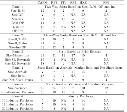
Sorts Based on Size, B/M, OP and Inv
Two-way Sorts
I start with two-way sorts based on size (the results can be found in Panel 1 of Table 2).
5
Model AS(BIC) RSW GRS AS(BIC) RSW GRS AS(BIC) RSW GRS Two-Way Sorts Based on Size, B/M, OP and Inv
Panel 1 Size-B/M Size-OP Size-Inv
CAPM 0.0 0.5 0 0.0 0.5 0.0 0 0.5 0
FF3 0.0 0.5 0 0.0 0.6 0.0 0 0.5 0
FF4 0.2 1.1 0 2.7 3.8 0.0 0 0.5 0
FF5 0.0 0.5 0 37.1 38.8 2.4 0 0.5 0
FF6 3.9 4.7 0 32.5 32.3 0.0 0 0.6 0
HXZ 0.0 0.5 0 23.8 24.7 6.5 0 0.5 0
Panel 2 B/M-OP B/M-Inv OP-Inv
CAPM 0.0 0.6 0.1 0.0 0.5 1.1 0.0 0.5 0.0
FF3 1.7 4.1 0.6 1.9 3.0 4.8 0.0 0.5 0.1
FF4 4.5 6.3 0.0 25.2 25.7 0.0 4.2 10.0 0.0
FF5 65.5 70.4 11.7 64.3 66.9 28.3 57.9 59.2 41.8
FF6 12.1 14.0 0.0 65.9 69.5 0.0 78.9 79.6 0.6
HXZ 39.5 40.2 1.4 33.8 32.5 11.0 40.5 41.0 21.0
Panel 3 Three-Way Sorts Based on Size, B/M, OP and Inv
Size-B/M-OP Size-B/M-Inv Size-Inv-OP
CAPM 0.0 0.5 0 0.0 0.5 0.0 0.0 0.5 0.0
FF3 0.0 0.5 0 0.0 0.5 0.0 0.0 0.5 0.0
FF4 0.9 1.9 0 1.8 2.5 0.0 0.2 0.7 0.0
FF5 3.5 5.0 0 1.7 2.8 0.5 0.2 0.9 0.0
FF6 15.8 18.0 0 30.6 35.2 0.0 3.9 4.8 0.0
HXZ 2.3 2.8 0 2.7 3.0 0.7 0.9 1.5 0.1
Table 2: Results for Sorts Based on Factors
The table displays results for factor-based sorts as test assets. The tests are based on monthly data from January 1975 to December 2016. For each set of regressions, the table
reports p-value for the AS test, the RSW test and the GRS test. All results are based on
10,000 bootstrap samples.
One would expect that the null should not be rejected for the FF5 and the FF6 models that
use exactly the same sort to construct factors, or for the HXZ model that relies on similar
indicators. For the portfolios based on the Size-OP the null hypothesis of mean-variance
efficiency indeed cannot be rejected for any of the three models when short sale constraints
are taken into account; however, if the short sale constraints are ignored, these models are
rejected as shown by the GRS test.
The portfolios with the high and positive alphas that lead to rejection are usually
some extent surprising given that small stocks are usually more short-sale constrained than
large stocks (see, e.g., Saffi and Sigurdsson (2010)), so one would expect that imposing the
short sale restriction should improve the performance of the asset pricing models. The high
alphas of microcaps are in line with the findings of Fama and French (2015a) that most
factor models struggle to explain the average returns of very small stocks.
For sorts that do not include size, the FF5, the FF6 and the HXZ models are not rejected
by the data (Panel 2). This finding holds independent of whether or not the short sale
constraints are taken into account for the FF5 and the HXZ but not for the FF6. In
particular, the six-factor model predicts negative alphas for stocks with high book-to-market
value but low operating profitability or low investment activity. The fact that the HXZ q
-factor model, which does not include a value -factor, performs on par with the five -factor
and the six factor models is in line with the findings of Hou et al. (2014a) and Fama and
French (2015b), who observe that this factor is redundant when controlling for investment
and profitability.
The more parsimonious models (FF3, FF4 and CAPM) are strongly rejected, suggesting
that they do not provide a good description of expected returns of these test assets. The only
exception is the original Fama-French three-factor model augmented with the momentum
factor is not rejected for the B/M-Inv sort under the short sale constraints, which may
suggest that adding momentum may implicitly capture some of the effects of the investment
factor. The rejection is not surprising given that these models do not include factors based
on profitability and investment.
Three-Way Sorts Based on Size, B/M, OP and Inv
The results for three-way sorts can be found in Panel 3 of Table 2. All models except for
the FF6 are rejected, or borderline rejected, at 5% level for all three way sorts (Panel 3).
Similar to the returns based on two-way sorts, this finding is driven by the microcaps. The
based on size, B/M and OP or size, B/M and Inv. The model struggles explaining high
returns of small stocks with low profitability and low investment activity.
Sorts Based on Anomalies
Model AS(BIC) RSW GRS AS(BIC) RSW GRS AS(BIC) RSW GRS
Panel 1 Sorts Based on Prior Returns
Size-Momentum Size-SR Reversals Size-LR Reversals
CAPM 0.0 0.5 0 0.0 0.5 0 0.0 0.5 0.1
FF3 0.0 0.5 0 1.8 3.0 0 1.9 2.5 2.8
FF4 0.3 0.7 0 25.6 25.2 0 4.0 5.0 0.0
FF5 0.0 0.5 0 12.9 14.3 0 42.1 41.8 10.7
FF6 2.5 3.0 0 44.8 44.4 0 50.4 52.1 0.7
HXZ 0.1 0.6 0 2.1 2.8 0 8.1 7.9 3.1
Panel 2 Sorts Based on Accruals, Market Beta and Net Share Issues
Size-Accruals Size-Beta Size-Net Share Issues
CAPM 0.1 0.6 0.0 0.0 0.5 0.1 0.0 0.5 0
FF3 0.0 0.5 0.0 5.2 5.9 4.1 0.0 0.5 0
FF4 8.9 9.2 0.1 3.8 4.5 0.0 0.1 0.8 0
FF5 0.0 0.5 0.0 49.4 51.0 4.5 0.0 0.5 0
FF6 4.2 4.8 0.0 17.2 17.2 0.0 2.5 3.0 0
HXZ 0.0 0.5 0.0 10.5 9.9 7.8 0.0 0.5 0
Panel 3 Sorts Based on Variance and Residual Variance
Size-Variance Size-Residual Variance
CAPM 0.0 0.5 0 0.0 0.5 0
FF3 0.0 0.5 0 0.0 0.5 0
FF4 0.0 0.5 0 0.3 0.7 0
FF5 1.1 1.7 0 1.0 1.5 0
FF6 0.5 1.0 0 2.2 2.7 0
HXZ 0.2 0.9 0 0.1 0.7 0
Table 3: Results for Sorts Based on Anomalies
The table displays p-values for sorts based on asset-pricing anomalies. The tests are based
on monthly data from January 1975 to December 2016. For each set of regressions, the
table reportsp-value for the AS test, the RSW test and the GRS test. All results are based
on 10,000 bootstrap samples.
The results for sorts based on anomalies can be found in Table 2.
We start by considering portfolios based on prior returns. The models that include
explicitly based on prior returns. However, the results are contradicting the expectations:
all models are rejected for the portfolios explicitly based on momentum itself. Again, the
biggest challenges are high expected returns of microcaps. The FF4, the FF5 and the FF6
are not rejected for portfolios based on short-term reversals if the short sale constraints are
taken into account. The FF5 and the FF6 are not rejected for portfolios based on long term
reversals. The fact that the FF5 that does not include momentum is not rejected seems to
support the view that the momentum is redundant.
All models struggle to explain low average returns of stocks with large accounting accruals,
with the possible exception of the FF4 withp-values slightly below 10% (Panel 2). Again,
the problem lies with size: the microcap portfolio in each accruals quintile has a very high
alpha.
The FF5 and the FF6 are not rejected for the portfolios based on beta. This finding suggest
that an additional ”low-beta” factor is redundant after profitability and investment activity
are taken into account.
All models are rejected for portfolios based on either variance or residual variance. Again,
the problem lays with microcaps: the portfolios based on small stocks with low variance
have a higher return than predicted by the models.
Industry Portfolios
All sets of portfolios based on industry strongly support the FF4 and the FF6 models that
are the only models including the momentum factor as can be seen from figure 4. Both
the FF5 and the HXZ can not explain high returns of the sector denoted as “HiTec” that
includes business equipment (computers, software, and electronic equipment). This suggests
Model AS(BIC) RSW GRS AS(BIC) RSW GRS AS(BIC) RSW GRS
Panel 1 Indsutry Portfolios
10 Portfolios 12 Portfolios 30 Portfolios
CAPM 0.3 0.8 16.5 0.4 0.8 12.7 0.5 0.9 40.3
FF3 0.0 0.5 1.0 0.0 0.5 0.7 0.1 0.6 5.8
FF4 14.8 15.7 1.7 20.5 20.7 0.2 69.9 70.3 0.1
FF5 0.3 1.7 4.5 1.4 2.4 1.8 2.9 4.7 9.2
FF6 22.9 23.0 1.8 31.2 31.4 0.0 84.8 88.8 0.1
HXZ 0.1 0.6 0.8 0.1 0.8 0.7 0.7 1.4 3.4
Table 4: Results for Industry Portfolios
The table displays p-values industry portfolios. The tests are based on monthly data from
January 1975 to December 2016. For each set of regressions, the table reports p-value for
the AS test, the RSW test and the GRS test. All results are based on 10,000 bootstrap samples.
1.5. Robustness Check: Transaction Costs
In this section, I consider the effect of transaction costs on the mean-variance efficiency.
While I incorporated short sale constraints, there are, of course, other market frictions that
may influence the results. In particular, some of the models above could have been rejected
due to the transaction costs.
Fortunately, the transaction costs can easily be incorporated into the null hypothesis as
follows:
H0 :αi ≤transactionCostsi ∀i= 1, . . . , N
H1 :αi > transactionCostsi for somei
(1.10)
The testing procedures discussed in chapter 3 can be applied to test the null hypothesis in
(1.10). This null is, again, constructed based on the assumption that the transaction costs
of factors are zero, which, of course, is not the case.
Estimating transaction costs is a non-trivial task as discussed by, for example, Novy-Marx
and Velikov (2015). It is thus difficult to determine the appropriate value of the transaction
the transaction costs needed to reject the model and try to determine whether they are
reasonable. For simplicity I set the transaction costs the same for each portfolio. Given
that the AS and the RSW tests produce similar results, I present the results only for the
AS test here.
CAPM FF3 FF4 FF5 HXZ FF6
Panel 1 Two-Way Sorts Based on Size, B/M, OP and Inv
Size-B/M 17 5 7 7 9 2
Size-OP 7 6 2 NA NA NA
Size-Inv 21 7 15 5 7 6
B/M-OP 14 3 3 NA NA NA
B/M-Inv 13 2 NA NA NA NA
OP-Inv 20 11 2 NA NA NA
Panel 2 Three-Way Sorts Based on Size, B/M, OP and Inv
Size-B/M-OP 41 10 5 5 5 NA
Size-B/M-Inv 21 8 3 2 3 NA
Size-Inv-OP 23 12 7 4 5 2
Panel 3 Sorts Based on Prior Returns
Size-Momentum 24 31 12 37 15 4
Size-SR Reversals 15 3 NA NA 5 NA
Size-LR Reversals 18 3 2 NA 1 NA
Panel 4 Sorts Based on Accruals, Market Beta and Net Share Issue
Size-Accruals 7 7 0 11 14 2
Size-Beta 18 1 2 NA 1 NA
Size-Net Share Issues 20 9 10 7 9 4
Panel 5 Sorts Based on Variance and Residual Variance
Size-Variance 49 24 28 7 10 12
Size-Residual Variance 50 19 13 5 9 5
Panel 6 Industry Portfolios
10 Industry Portfolios 6 10 NA 8 14 NA
12 Industry Portfolios 5 10 NA 8 14 NA
30 Industry Portfolios 5 8 NA 4 8 NA
Table 5: Required Transaction Costs
The table displays levels of transaction costs in basis points, so that the model cannot be rejected by the AS test at the 10 percent level, respectively. The tests are based on monthly data from January 1975 to December 2016. All results are based on 10,000 bootstrap samples.
Table 5 presents levels of transaction costs in basis points, so that the AS test does not
costs below 17bps are needed to reject the CAPM and only below 5bps to reject the FF3.
If the model can not be rejected at the 10 percent level, no matter how low the transaction
costs are, I put “NA”. “NA”s, of course, correspond to the p-Values higher than 10% in
chapter 3.
In order to judge whether the required transaction costs are reasonable, I’ll use the estimates
by Novy-Marx and Velikov (2015) as a benchmark. In particular, they estimate that the
transaction costs for strategies with low turnover and annual re-balancing (such as strategies
based on size, value, profitability, investment or accruals) are usually around 4-10bps. The
transaction costs for mid-turnover strategies with monthly re-balancing such as momentum,
long term reversals, net share issuance or volatility usually average between 20-50 bps.
Finally, for high turnover strategies such as short term reversals the costs are often higher
than 150bps. For example, the CAPM requires the transaction costs of 20bps to explain the
alphas on OP-Inv strategies, while the real transaction costs are likely to be below 10bps.
Based on these estimates, the CAPM and the FF3 would probably be rejected even after
transaction costs are taken into account because these models require relatively high costs
for presumably cheap strategies (such as two- or three-way sorts). These two models also
need high transaction costs in order to be not rejected relative to other models. On the
other hand, the FF6 always requires relatively low transaction costs. The highest value is
12bps for size-variance sort, which is a high turnover strategy and thus probably has indeed
very high transaction costs. This suggests that the FF6 may sometimes be rejected solely
due to the presence of transaction costs.
1.6. Conclusion
I examine the implications of mean-variance efficiency in linear factor models under
con-sideration of short sale restrictions and explore two testing procedures to test the validity
of these models when such restrictions exist. I employ two moment inequality tests, and
tests have slightly better power when compared to the RSW test, but their performance
is very similar. Empirically, these two types of tests produce the same qualitative results.
In the empirical study, I apply the two types of tests to explore the validity of multiple
linear asset pricing models. The results indicate that some model specifications, such as the
Fama-French five factor model augmented with the momentum factor, are able to explain
several of the widely known asset pricing anomalies if we allow for possible mis-pricing due
1.7. Appendix
1.7.1. Conditionally Heteroscedastic Errors
I re-run the simulation for the dimensionality N = 10 using conditionally heteroscedastic
errors. The simulated processes follow a constant conditional correlation GARCH model,
which consists of 10 univariate GARCH(1, 1) processes related to one another with a
con-stant conditional correlation matrix. The coefficients of univariate GARCH processes are
set equal to the estimates obtained from the returns of ten industry portfolios. The GARCH
processes are standartized, so that the unconditional variance of each process is equal to
one. The correlation matrices are the same as before.
N = 10
Test Distr H0/H1 ΩN eg ΩZero ΩP os
AS Normal H0 6.5 5.6 6.1
RSW Normal H0 5.6 5.2 5.5
AS t3 H0 6.6 6.1 6.6
RSW t3 H0 6.0 5.6 6.1
AS Normal H1 58.1 64.8 79.3
AS(size-adj) Normal H1 54.9 64.1 77.9
RSW Normal H1 50.2 56.6 76.0
AS t3 H1 63.8 67.9 80.5
AS(size-adj) t3 H1 62.3 66.8 78.9
RSW t3 H1 56.1 60.1 77.7
Table 6: Simulation for Mean Test with GARCH Disturbances
Sample size isT = 500, dimensionality is N = 10. Based on 5,000 Monte-Carlo repetitions
underH0and 10,000 underH1. Critical values are computed using 3,000 bootstrap samples.
The nominal significance level is 5%. AS(size-adj) denotes size-adjusted version of the AS test under the adjusted nominal significance level, so that the empirical MNRP matches that of the RSW test.
The results reported in Table 6 show that both tests are robust to conditional
heteroscedas-ticity. The resulting average power and the empirical MNRP are essentially the same as for
the simulation without conditional heteroscedasticity. The only exception is the
slightly lower power under the heteroscedastic errors. This finding implies that both tests
are robust under conditional heteroscedasticity although they don’t explicitly account for
CHAPTER 2 : International Return Predictability
2.1. Introduction
Assessing the predictability of the equity premium is one of the fundamental problems in
the financial literature.1 However, despite years of research, there is no consensus about
whether the equity premium is predictable, how much it varies over time and which variables
can be used to predict it.2
International markets provide rich data that can be used to deepen our understanding of
return predictability. However, most studies of international return predictability examine
each capital market separately. Most come to the conclusion summarized by Schrimpf (2010)
that “return predictability is neither a uniform, nor a universal feature across international
markets”.3 The inconclusive evidence of international predictability may be driven in part
by the noise in the data. Due to arbitrage considerations, if predictability exists, then
it is likely to be weak.4 Thus, an efficient estimation method is required to assess the
predictability of international equity premium. Although it would be more efficient to
consider international capital markets jointly, rather than examining each one in isolation,
the literature doing so is lacking.
In this chapter, I investigate patterns of equity premium predictability in international
capital markets and explore the robustness of common predictive variables. In particular,
I focus on predictive regressions with multiple predictors. To obtain precise estimates, two
estimation methods are employed. First, I consider all capital markets jointly as a system
of regressions. Second, I take into account uncertainty about which potential predictors
forecast excess returns.
1Henceforth, I use the words “equity premium” and “return” interchangeably as standard in the literature. 2
See a survey by Cochrane (2011).
3Multiple papers explore each capital market individually such as Ang and Bekaert (2002), Rapach et al.
(2005), Schrimpf (2010), Neely and Weller (2000), Paye and Timmermann (2006), Giot and Petitjean (2006) among others.
4Wachter and Warusawitharana (2009) and Wachter and Warusawitharana (2015) explore how the prior
I treat the data as seemingly unrelated regressions (SUR), first introduced by Zellner (1962).
Country-specific regressions widely used in earlier literature ignore the fact that excess
returns are contemporaneously correlated across countries and treat the covariance matrix
of residuals as diagonal. SUR exploits this correlation to increase the estimation precision.
I assume that an investor is uncertain about which potential predictors to include in the
predictive regression, which contradicts the typical assumption that the investor chooses a
set of predictors a priori. The assumption of model uncertainty is justified given the large
number of potential predictors in the literature and the limited consensus about which of
them forecast returns. Existing pricing theories offer little guidance about which
predic-tors should be included in the regression, so the decision regarding the predictive power
of potential regressors is often based on empirical studies, making the predictability
evi-dence subject to data-snooping concerns.5 The international investor is likely to face an
even higher degree of model uncertainty because most empirical studies focus only on the
U.S. market. Therefore, prevailing views are likely to be biased toward regressors deemed
significant for the U.S.6 It is, therefore, necessary to take model uncertainty into account
when evaluating the statistical evidence in favor of return predictability.
I use the Bayesian spike-and-slab approach to incorporate model uncertainty.7 The
expres-sion “spike-and-slab” refers to the prior imposed on the coefficients. The prior represents a
mixture of two normal distributions: the spike, which is centered very tightly around zero,
and the slab, which represents a very flat distribution. The frequency, with which a
partic-ular predictive variable is estimated to be a draw from the slab distribution, can be used
to estimate the inclusion probability. A fundamental property of this approach is selective
shrinkage. The posterior means of coefficients that are found to be non-informative of
fu-ture returns is strongly shrunk toward zero,thereby reducing estimation error. On the other
5
This concern was raised by Welch and Goyal (2007), Ferson et al. (2003) and Bossaerts and Hillion (1999) among others.
6
Dimson et al. (2008) argues that the strong performance of the U.S. market is unique; thus, focusing solely on the U.S. may have consequences similar to selection bias.
7
hand, the posterior means of the coefficients that predict equity premium is only slightly
shrunk to zero if at all.
The spike-and-slab approach has not been previously used in the context of return
pre-dictability. The classical approach to model uncertainty is Bayesian model averaging as
in Avramov (2002), Cremers (2002), and Schrimpf (2010). The Bayesian model averaging
approach assigns posterior probabilities to all candidate model specifications and uses these
probabilities as weights on the individual models to obtain a composite model used for
forecasting. The weakness of this approach is that it requires considering all possible
mod-els, which is computationally infeasible in the context of international return
predictabil-ity. In this chapter, I consider ten countries with six potential regressors, which yields
260 = 1.15×10¹⁸ models. In contrast, the spike-and-slab method uses Gibbs sampling to
identify models with a high probability of occurrence.
I re-examine both in- and out-of-sample evidence of predictability for ten international
capital markets. In particular, I explore the importance of dividend-price ratio, four interest
rate variables and inflation. As a result, several conclusions emerge about international stock
return predictability.
First, I find that variables that are statistically significant predictors in the country-specific
regressions are insignificant when the capital markets are studied jointly. In particular, the
consensus in the literature is that interest rates are among the most robust predictors for
international equity premium, while the valuation ratios and, in particular, the
dividend-price ratio do not predict returns.8 However, my results suggest that the in-sample evidence
in favor of the interest rate variables is spurious and is mostly driven by ignoring the
cross-country information. Conversely, the dividend-price ratio emerges as the only robust
predictor of future stock returns. I, thus, show that ignoring the cross-correlation of errors
could lead to erroneous inferences about the relevance of predictive variables.
8