PERFORMANCE ANALYSIS AND OPTIMIZATION OF AN M/M/3 QUEUEING SYSTEM UNDER TETRAD POLICY

433 | P a g e

PERFORMANCE ANALYSIS AND OPTIMIZATION

OF AN M/M/3 QUEUEING SYSTEM UNDER

TETRAD POLICY

Anupama

, Anjana Solanki

1

Research Scholar,Deptt of mathematics ,GBU, Gr. Noida, (India)

Professor and Head, Deptt of mathematics, GBU, Gr. Noida,( India)

ABSTRACT

In this paper, we consider machine repair problem with three removable repairmen which is adjusted one at a

time depending upon the number of broken machines in the M/M/3 queueing system with finite capacity L

operating under the tetrad policy. In this system, the repairman is not available for serving the failed units,

when the number of failed units is less than N. We derive the probability generating function (PGF) of the

number of failed units waiting in the system. The total expected cost function per unit time is derived to

calculate the operating optimal tetrad policy at minimum cost. Along with this Sensitive analysis and direct

search algorithm on the optimum value also performed.In the end, some numerical examples are presented to

show the influence of the system parameters on performance measures.

Keywords: Broken Machines, Cost Control. Tetrad Policy, M/M/3 Queueing System

1.

INTRODUCTION

We consider an M/M/3 queuing system where the number of operating service stations (or repairmen) can be adjusted one at a time at customer's arrival or service completion epochs depending on the number of failed units present in the system under steady-state conditions. Hahn and Sivazlian [4] introduced this model for M/M/2 at the indistinguishable service stations. The concept of a (0, N) policy in the controllable M/M/Isystem was first introduced by Yadin and Naor [8]. An operating policy is called the (0, N) policy if the number of customers in the system reaches N, where N 1 for the first time after the server is removed from the system,

the server returns immediately and provides service until there are no customers present in the system. Bell [1], Magazine [9], Sobel [10], and others concentrated on developing the optimal operating policy of the controllable systems under various assumptions regarding the distributions of interarrival and service times.

Gnedenko et al. [3] had studied the reliability of a single-server 2-unit warm standby system with exponential failure and general repair time distributions. Gopalan [7] investigated the reliability of a single-server n-unit system with (n- 1) warm standbys with an exponential failure time distribution and two types of general repair time distributions of the operating unit and of the standbys.

434 | P a g e

iii. To formulate the total expected cost function for the system, and determine the optimal value of the control parameter N.

iv. To carryout sensitivity analysis on the optimal value of N and the minimum expected cost through numerical illustrations.

2. DESCRIPTION OF THE MODEL

2.1. DEFINITION OF THE OPERATING POLICY:

The special feature of operating policy of this M/M/3 queuing system of finite capacity L under the tetrad policy is that the number of the operating repairmen can always be adjusted based on the

number of broken machines in the system. Thus, the number of broken machines in the system is monitored at every new failed machine's arrival and service completion epochs. Whenever there are no failed machines in the system, repairmen are in vacations temporarily, and may not be reactivated until certain condition is satisfied. We discuss the states of the system by the pairs (i, n), i = 0, 1, 2, 3, n = 0, 1, 2,…Q,…R,…N,…M,…K,…L, where i = 0 denotes that the repairmen are on temporally vacations, i = 1 denotes that one of the repairmen working in the system, i = 2 denotes that two of the repairmen working in the system, i = 3 denotes that all the three repairmen are active and working in the system and n is the number of failed machines in the system.

2.2 EQUATIONS GOVERNING THE SYSTEM:

Consider the probabilities used in the system

P(0,n) = probability that the there is no active repairmen in the system and there are n customers in the system, where n = 0, 1, 2, 3,…N-1,

P(1,n) = probability that the there is one active repairmen in the system and there are n customers in the system, where n = 0, 1, 2, 3,…

Q,…R,…N,…M-1,

P(2,n) = probability that the there is two active repairmen in the system and there are n customers in the system, where n = Q + 1, Q + 2,…R, R + 1, ….N,…M,…K-1,

P(3,n) = probability that the there is three active repairmen in the system and there are n customers in the

system, where n =

2.3 NOTATIONS :

λ = arrival rate exponentially distributed, μ = service rate exponentially distributed,

F0(z) = probability generating functions, when there is no active repairmen in the system,

F1(z) = probability generating functions, when there is one active repairmen in the system,

F2(z) = probability generating functions, when there is two active repairmen in the system,

F3(z) = probability generating functions, when there is three active repairmen in the system,

P0 = probability that all the repairmen are on vacation,

P1 = probability that one of the repairmen is active and working in the system,

P2 = probability that two of the repairmen are active and working in the system,

P3 = probability that all the repairmen are active and working in the system,

435 | P a g e

L1 = the expected number of failed machines in the system when any one of the repairman working in the

system,

L2 = the expected number of failed machines in the system when two of the repairmen working in the system,

L3 = the expected number of failed machines in the system when all the three repairmen working in the

system,

Ls = the expected number of failed machines in the system,

Ch = holding cost per unit time per failed unit present in the system,

Cv1 = holding cost per unit time when one repairman is on vacations,

Cv2 = holding cost per unit time when two repairmen are on vacations,

Cv3 = holding cost per unit time when all the repairmen are on vacations,

C01 = cost of one repairman working in the system per unit time,

C02 = cost of two repairmen working in the system per unit time,

C03 = cost of three repairmen working in the system per unit time,

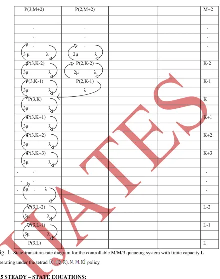
2.4 STATE- TRANSITION-RATE DIAGRAM

The probabilities P( i, n) where i = 0, 1, 2, 3 and n is the number of failed unit in the system, of the arrival and departure of the served unit are shown through the state-transition diagram for the controllable M\M\3 queueing

system with finite capacity L under the tetrad policy.

Number of working servers

3 2 1 0

P(0,0) 0 μ λ

P(1,1) P(0,1) 1

µ λ λ

P(1,2) P(0,2) 2

. . λ .

. . .

. . .

. μ λ λ

P(1,Q-1) P(0,Q-1) Q-1

µ λ λ

2µ P(1,Q) P(0,Q) Q

µ λ λ

P(2,Q+1) P(1,Q+1) P(0,Q+1) Q+1 2µ λ μ λ λ

P(2,Q+2) . . .

436 | P a g e

. . . .

2µ . λ μ λ λ

P(2,R-1) P(1,R-1) P(0,R-1) R-1 2µ λ µ λ λ

3µ P(2,R) P(1,R) P(0,R) R

2µ λ µ λ λ

P(3,R+1) P(2,R+1) P(1,R+1) P(0,R+1) R+1

3µ λ 2µ λ µ λ λ

P(3,R+2) P(2,R+2) P(1,R+2) P(0,R+2) R+2

3µ λ 2µ λ μ λ λ

. . . . .

. . . . .

. . . . .

3µ λ 2µ λ μ λ λ

P(3,N-2) P(2,N-2) P(1 N-2) P(0,N-2) N-2 3µ λ 2µ λ µ λ λ

P(3,N-1) P(2,N-1) P(1,N-1) P(0,N-1) N-1

3µ λ 2µ λ µ λ λ

P(3,N) P(2,N) P(1,N ) N

3µ λ 2µ λ µ λ

P(3,N+1) P(2,N+1) P(1,N+1) N+1

3µ λ 2µ λ µ λ

P(3,N+2) P(2,N+2) P(1,N+2) N+2

3µ λ 2µ. λ μ λ

. . . .

. . . .

. . . .

3µ λ 2µ λ μ λ

P(3,M-3) P(2,M-3) P(1,M-3) M-3

3µ λ 2µ λ µ λ

P(3,M-2) P(2,M-2) P(1,M-2) M-2

3µ λ 2µ λ µ λ

P(3,M-1) P(2,M-1) P(1,M-1) M-1

3µ λ 2µ λ λ

P(3,M) P(2,M) M

3µ λ 2µ λ

P(3,M+1) P(2,M+1) M+1

437 | P a g e

P(3,M+2) P(2,M+2) M+2

. . .

. . .

. . .

3 µ λ 2µ λ

P(3,K-2) P(2,K-2) K-2

3µ λ 2µ λ

P(3,K-1) P(2,K-1) K-1

3µ λ λ

P(3,K) K

3µ λ

P(3,K+1) K+1

3µ λ

P(3,K+2) K+2

3µ λ

P(3,K+3) K+3

3µ λ

. . .

. . .

. 3µ . λ .

P(3,L-2) L-2

3µ λ

P(3,L-1) L-1

3µ λ

P(3,L) L

Fig. 1.

operating under the tetrad policy

2.5 STEADY – STATE EQUATIONS:

The transition-state diagram for the steady state problem of the controllable M/M/3system with finite capacity

and three removable servers under the tetrad policy is shown in Fig. 1. The steady state

probabilities equations governing the model are obtained as follows:

(1)

(2)

438 | P a g e

(4)

(5)

(6)

(7)

(8)

(9)

(10)

(11)

(12)

(13)

(14)

(15)

(16)

(17)

(18)

(19)

(20)

(21)

Equations (1)–(21) can be solved by using recursive method for the P(i,n) (i = 0, 1, 2, 3)

, 1≤ n ≤ N-1 (22)

1

439 | P a g e

Where

3. THE GENERATING FUNCTIONS

The Generating function techniques applied to obtain analytic solutions P(i,n) (i = 0,1,2,3) in closed form expressions.

Partial probability generating functions are as follows:

4. PERFORMANCE CHARACTERISTICS OF THE SYSTEM:

In this section we obtain some performance characteristics using generating functions derived in previous section.

440 | P a g e

THE EXPRESSIONS ARE L

, L

, L

,L

AND L

L0 = [ (z)]z=1 = (30)

Similarly, we can find L1 we calculate [ (z)]z=1 using L’Hospital’s rule twice to obtain

similarly

Hence we can easily obtain the expected number of customers in the system from (30)-(33) \

441 | P a g e

5. EXPECTED TOTAL COST FUNCTION

In this section we calculate the total expected cost function per unit time for the controllable M\M\3 queueing

system with finite capacity L operating under the tetrad policy, in which

are decision variables. Along with our objective to determine the optimum value of the control parameters say ( , ), so as to minimize the cost function , we also constructed the cost

structure.

The total expected cost function per unit time is given by

As the total expected cost function is highly non linear and complex, it is extremely difficult to determine the optimal values ( , ), analytically which minimize the total expected cost function per unit time.

Direct search method may use to obtain useful results. In Direct search algorithm, it is compulsory to have upper bounds for decision variables and direct search algorithm can be terminated after obtaining a global optimum in

the interior region. Here L is the upper bounds of the decision variables for obtaining the

optimal values ( , ). Following are the steps in the direct search algorithm.

5.1 Find the optimal values ( ) for fixed Q ie.

5.2 Find the set of all minimum cost solutions for Q = 1, 2,…L-4 ie

Φ =

5.3 Find the optimal value Q*, ie.

The computer software MATLAB is used for computer programming. Let the system capacity is L = 20 & the fixed cost for every lost customer Cl = $50.

Now, we use sensitivity analysis on the optimum value based on changes in specific values of the system parameters λ and μ. The following cost elements are used:

Case I: = $10, = $10, , C03 = $30, Cv = Cv1+ Cv2+ Cv3 = $30

Case II: Ch = $15, = $10, , C03 = $30, Cv = Cv1+ Cv2+ Cv3 = $30

Case III: Ch = $10, = $15, , C03 = $45, Cv = Cv1+ Cv2+ Cv3 = $30

Case IV: Ch = $10, = $10, , C03 = $30, Cv = Cv1+ Cv2+ Cv3 = $45

Case V: Ch = $10, = $10, , C03 = $30, Cv = Cv1+ Cv2+ Cv3 = $30

442 | P a g e

and its minimum expected cost F

for the above five cases are shown in Table A and Table B for various values of (λ,μ).

(For fixed value of λ=4)

The Expected cost

(λ,μ) (4,5) (4,6) (4,7) (4,8) (4,9) (4,10)

Case I (2,3,4,5,6) (3,4,5,6,7) (3,4,5,6,7) (3,4,5,6,7) (3,4,5,6,8) (4,5,6,7,8)

99.57 101.23 103.31 105.14 106.12 107.59

Case II (1,2,3,4,5) (1,2,3,4,5) (1,2,3,4,5) (2,3,4,5,6) (2,3,4,5,6) (2,3,4,5,6)

144.21 146.35 149.73 151.64 153.81 155.60

Case III (2,3,4,5,6) (3,4,5,6,7) (3,4,5,6,7) (3,4,5,6,7) (3,4,5,6,8) (4,5,6,7,8)

107.67 108.22 110.34 112.26 113.49 114.73

Case IV (2,3,4,5,6) (3,4,5,6,7) (3,4,5,6,7) (3,4,5,6,8) (3,4,5,6,9) (4,5,6,7,8)

104.52 107.21 111.32 114.69 117.74 120.54

Case V (4,5,6,7,8) (5,6,7,8,9) (5,6,7,8,9) (6,7,8,9,10) (6,7,8,9,10) (6,7,8,9,10)

126.52 132.43 137.35 142.61 151.78 153.67

Through the analysis of Table A, we observed that

(a) F increases as μ increases in all the cases.

(b) slightly changes as μ increases.

(c) decreases as Ch increases.

(d) are almost the same for case 1, case 3, case 4 intuitively. C01, C02,

C03 and Cv rarely affect the optimal values of

(For fixed value of μ=7)

The Expected cost

(λ,μ) (1,7) (2,7) (3,7) (4,7) (5,7) (6,7)

Case I (2,3,4,5,6) (2,3,4,5,6) (3,4,5,6,7) (3,4,5,6,7) (3,4,5,6,7) (3,4,5,6,7)

74.62 96.51 97.64 101.23 103.52 105.34

Case II (1,2,3,4,5) (2,3,4,5,6) (2,3,4,5,6) (2,3,4,5,6) (2,3,4,5,6) (2,3,4,5,6)

101.67 124.79 136.81 142.90 151.87 156.92

CaseIII (2,3,4,5,6) (2,3,4,5,6) (3,4,5,6,7) (3,4,5,6,7) (3,4,5,6,7) (3,4,5,6,7)

82.62 94.23 104.34 112.11 117.83 123.97

Case IV (2,3,4,5,7) (2,3,4,5,7) (2,3,4,5,8) (3,4,5,6,7) (3,4,5,6,7) (3,4,5,6,7)

443 | P a g e

Case V (3,4,5,6,8) (4,5,6,7,8) (5,6,7,8,9) (5,6,7,8,9) (5,6,7,8,9) (4,5,6,7,8)

106.58 126.83 134.09 136.11 138.34 139.31

Through the analysis of Table B, we observed that

(e) F increases as λ increases in all the cases.

(f) slightly changes as λ increases.

(g) decreases as Ch increases.

(h) are almost the same for case 1, case 3, case 4 intuitively. C01, C02,

C03 and Cv rarely affect the optimal values of .

6. CONCLUSIONS:

In this paper we derived the analytic steady-state results for the controllable M\M\3 queueing system with finite

capacity operating under the tetrad policy. Sensitivity analysis between the optimal value of

and the specific values of λ and μ and the cost elements Ch, C01, C02, C03 and Cv. It is also

noticed that C01, C02, C03 and Cv rarely affect the optimal values of and Ch affected the optimal

values slightly.This paper is the generalization of the ordinary M\M\2 queueing system and the N-policy M\M\1

queueing system. Finally, a cost model is evaluated to determine the optimal level

of failed machines in the system

.

REFERENCES:

[1]. Bell CE,” Characterization and computation of optimal policies for operating an M/G/1 queueing system with removable server”. Operations Research 19:208–218 (1971).

[2]. Bell CE,”Optimal operation of an M/G/1 priority queue with removable server”. Operations Research

21:1281–1289, (1972).

[3]. Gnedenko et al.” Mathematical methods of Reliability Theory” Academic press, New York, .(1969).

[4]. Hahn and Sivazlian,”Distribution of the busy period in a controllable M\M\2 under the Triadic (0‚K‚N‚M) policy”, J. Appl. Prob., Vol. 27, pp.425-432,(1990).

[5]. K. H. Wang and B. D. Sivazlian.” Reliability of a system with warm standbys and repairmen”.

Microelectron. Reliab, 29, 849-860 (1989).

[6]. Kuo-Hsiung Wang and Ya-Ling Wang,” Optimal control of an M/M/2 queueing system with finite capacity operating under the triadic (0‚Q‚N‚M) policy” Math Meth Oper Res 55:447–460, (2002).

[7]. M. N Gopalan,” Probablistic analysis of single server n-unit system with (n-1) warm standbys.” Oper Res.

23, 591-595, (1975).

444 | P a g e

[9]. M. J. Magazine,” Optimal control of multi-channel service systems”. Naval Res. Logist. Q. 177-183 (1971). [10].M. J. Sobel,” Optimal average-cost policy for a queue with start-up and shut-down costs". Opns Res. 17,