Theoretical Study of the Behavior of a Hydraulic Ram Pump with Springs System

Theoretical Study of the Behavior of a Hydraulic Ram

Pump with Springs System

Andriamahefasoa Rajaonison*, Hery Tiana Rakotondramiarana

Institute for the Management of Energy (IME), University of Antananarivo, Antananarivo, Madagascar

Abstract

A new type of hydraulic ram pump, called "Raseta pump", was invented, patented and crafted in Madagascar. The peculiarity of this hydram pump over conventional ones is that there is a spring in each of the waste and delivery valves. In addition, the usual air balloon is replaced by a balloon with 4 springs. Thus, this paper aims at theoretically studying the behaviour of this hydram pump equipped with a system of springs. For that purpose, a model associated with the studied hydram pump was developed and coded on Matlab. Then, a global sensitivity analysis was carried out for identifying the most influential parameters of this model while successively considering as the surveyed model outputs: the amount of wasted water, the amount of pumped water and the efficiency of the pump. As results, the most dominating parameters are relatively the same as those found by previous works on the conventional hydram pump without springs: height of the water column in the delivery pipe, the height of supply tank, the weight of the waste valve, and the length of the waste valve stroke. However, there are 3 other parameters that the present study exceptionally found as among the most influential ones as well, namely: the stiffness of the spring in the waste valve, the modulus of elasticity of the fluid, and the radius of the waste valve disk. In addition, similar to the case of air balloon, the effect of the spring balloon is not relevant. An extension work could be a techno-economic investigation of a pump system constituted by a number of hydram pumps similar to the one studied here for increasing water head in a pico hydropower plant.

Keywords

Hydram pump, Water supply, Bernoulli equation, Raseta pump, Modelling, Global sensitivity analysis

1. Introduction

The hydraulic ram pump, which is simply called hydram pump from now on, was invented by Joseph Michel Montgolfier by the end of the 18th century [1]. Used as a water supply machine, this pump uses the energy of water to raise a certain water amount to a height much higher than that of the initial watercourse [1]. This process is based on a phenomenon known as "water hammer" [2] which is a shock wave created by the sudden stop of moving water [3]. In other words, the kinetic energy of a water column having taken a certain speed is stopped suddenly by a valve which creates an overpressure [4, 5]. This harmful phenomenon for pipelines [6] is used in the hydram pump to raise water without any other source of energy than that of the water itself [7].

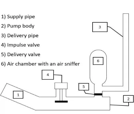
Several studies were carried out on hydram pump which generally has six main components [5, 8, 9] as can be seen from Figure 1.

* Corresponding author:

rajmahefasoa@gmail.com (Andriamahefasoa Rajaonison) Published online at http://journal.sapub.org/ajfd

Copyright©2019The Author(s).PublishedbyScientific&AcademicPublishing This work is licensed under the Creative Commons Attribution International License (CC BY). http://creativecommons.org/licenses/by/4.0/

Figure 1. Components of a conventional hydram pump

cycle was then divided into six distinct periods and the relationship between speed and time for the water column in the supply pipe during each part of the cycle was determined. It was concluded that the height of the discharge tank and the speed required to start closing the water valve have significant effects on the amount of pumped water and lost water per cycle as well as the cycle time. More precisely, it was found that, for discharge pressures less than half the maximum pressure that can be developed by the hydram pump, the amounts of pumped water and lost water per cycle can respectively be predicted with an error of less than 10%, for a particular setting of the ram valve. The values given by the mathematical results are much closer to the experimental values for the largest ram. Meanwhile, Gibson [4] considered a cycle in four periods and showed that the amount of lost water mostly depends on the mass and the stroke of the waste valve, the ratio between the length of the supply pipe, and the height of the supply tank while Young [9] asserts that this last parameter affects only the total duration of a cycle. The pump capacity and efficiency are influenced by: the waste valve surface, the delivery height, the ratio of the delivery height to the supply height, and the ratio between the length of the supply pipe and the height of the supply tank. According to Gibson [4], the area of the waste valve is the most important source of loss and contributes between 15 and 25% of the total energy received by the pump. It was also showed that it is impossible to pump at a delivery height greater than about six times the supply height. Another study on the hydram pump was conducted by Kahangire [5] in which friction losses are considered. Flux returns and the effects of the elasticity of valve materials are neglected. The pumping cycle is divided into four main periods, based on the position of the waste valve and the average time-velocity variation in the supply pipe. The developed model is based on the following assumptions: an one-dimensional approximate equation of steady flow is applied for flow in the supply pipe; the parameters determined under constant flow conditions are approximately constant; the closing of the waste valve is instantaneous; the water velocities in the supply pipe when the waste valve begins to close and is finally closed are the same; the resistance due to the movement of the spindle through the valve guide is negligible and constant; only the changes of the flow average speed and the pressure difference in the system are taken into account. Kahangire [5] mentions that pump efficiency, pumped water flow and pump power are influenced by: the length of the supply pipe [8, 10]; length of stroke, mass and size of the waste valve; and finally, the supply height [11]. For the air chamber, its volume has no significant effect on the operating characteristics of the pump but may be necessary to absorb the increased pressures that occur in the pump [5]. Inthachot et al. [12] aimed to build a reliable and cheap ram made of commercially available parts and available locally. They were able to deduce that from a certain size; the volume of the air chamber is not crucial for the operation of the ram. Each valve had a different spring, and both show that the tension of their springs greatly

influences the performance of the pump [12]. For Deo et al. [13] they presented a design methodology of the pump by doing an analysis on the ANSYS (Computational Fluid Dynamics) CFD- FLUENT R14.5software [14]. They concluded that the parameters that are essential for the efficiency and design of the pump are: the static pressure in the supply head, the diameter of the supply pipe [15], the size of the air chamber, and the waste valve [13, 16]. Girish et al. [17] have done a study of the pump to analyse the flow and the height of the delivery. They have shown that flow and head are strongly influenced by: the height, length and diameter of the supply pipe [15, 18], and the discharge pipe. As before the chamber eliminates the sound of water hammers [17]. In addition, Hussin et al. [19] analysed and developed a ram pump to achieve a desired delivery height of up to 3 meters with reduced operating cost. The simulation was performed using the ANSYS CFX R15.0 software [20]. The results of this study show the diameter of the air chamber is critical to increase the water pressure. In addition, the supply height and the amount of water at the source play a vital role in the system [19].

In summary, it has been shown that the efficiency of the pump is intrinsically linked to the supply height, the stroke and the mass of the waste valve, the volume of the air chamber [21] and finally the height of the delivery tank.

At my present state of knowledge, no study has been conducted on the modelling of a hydram pump with a spring system at the waste valve and the delivery valve. As for the air chamber equipping the conventional hydram pump, it is replaced by a balloon with 4 springs attached to a valve at their ends (Figure 3).

Thus, the objective of the present work is firstly to develop a model of this hydram pump with spring system then to carry out a global sensitivity analysis of the abovementioned model.

2. Materials and Methods

2.1. Description of the Functioning of Hydram Pump System to Model

Figure 3. Scheme of the studied hydram pump with system of springs [22]

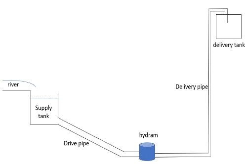
The hydram is fed by a source which is a tank or stabilization tank itself fed by a river, a watercourse, etc. The pumped water is then stored in a tank for later use (Figure 2). The operation of the pump can be described in a cycle of 6 periods [1] (Figure 4).

Figure 4. Functioning of the studied hydram pump

Period 1 is the time during which the waste valve begins to close until it is completely closed [5, 7, 12] (Figure 4a) (Figure 4b). Then, in period 2 is the moment between the full

closure of the waste valve and the opening moment of the delivery valve [21] (Figure 4c). The third period is the time during which the delivery valve remains open [5, 21] (Figure 4d). This is followed by the fourth period, which is the time between the closing of the delivery valve and the beginning of the opening of the waste valve [21] (Figure 4e). Then during period 5, it is the time between the beginning of the opening of the waste valve and the start of the water loss (Figure 4e and Figure 4f). And finally, during period 6, it is the time between the beginning of losses and the moment when the waste valve starts to close (figure 4g). Once the sixth period is over, the cycle restarts.

2.2. Mathematical Formulation

A step-by-step analysis will assist in establishing the model that gives the amount of lost water, the amount of pumped water per cycle, and the efficiency of the hydram pump.

2.2.1. Simplifying Assumptions

The following simplifying assumptions are adopted for modelling the studied hydram pump:

I. The quantity of water in the supply tank is constant, that is, the flow of water entering it from a river, or any other form of watercourse is greater than the flow of water coming out through the supply pipe. An overflow is also installed.

II. The waste valve is assumed to be elastic [1]. III. The 4 springs in the balloon are identical and the sum

of their masses is neglected.

IV. The initial position of the valve in the balloon is at the same level as that of the waste valve.

V. The weight of the delivery valve is negligible compared to the return force of its spring.

VI. The supply pipe has no obstacle such as a fitting, a bend or other obstacles. The head loss in the supply pipe is only due to the roughness of the pipe. VII. In the study of period 2, the friction in the supply

pipe is neglected because the pressure change caused by this friction is not significant compared to the other pressure changes for a well installed pump [1]. VIII. The waste valve disk is considered to be a circular plate whose bending is assumed as being due to a point load applied to its centre.

IX. The disk of the waste valve is assumed to rest all around its circumference.

X. Frictions during study of period 5 are neglected [1] XI. The valve attached to the ends of the springs in the

balloon is well sealed so that no water can overflow outside during operation of the studied hydram pump.

XII. The air in the balloon containing the four springs is in contact with the outside air.

XIII. The head loss at the elbow at the base of the hydram pump is neglected.

of the period 3 is instantaneous and, therefore, does not influence the duration of a cycle.

2.2.2. Mathematical Model Relating to Period 1

Period 1 represents the duration (s) of the closure of the waste valve [21] and is determined by equation (1):

3 1 w H v A 2 c r 2 L b 4 i k 1 v M 1 H 2 g 4 w v A g v M 0 S L 1 t                                  ( (1)                                 

 00254

0 S 85 6 52 0 10 0254 0 0 S 275 0 345 0 0 S 0254

0 . . .

. . . .

 _{[21] (2)}

In addition, apart from the nomenclature given in the appendix 1, b represents, in equation (1), the linear head loss coefficient of the supply pipe (-). More precisely, b can be calculated with the help of the formula of Poiseuille, Blasius or Blench according to the flow regime in the supply pipe [18, 23, 24, 25, 26]; hence, the calculation of b requires the knowledge of the value of the water minimum velocity v0 at which the waste valve begins to close (m.s-1) [21] and which can be computed by equation (3) :

c s H g 2 0

v  (3)

                  _              

 00254

0 S 30 13 95 0 10 0254 0 0 S 06 1 43 2 0 S 0254 0 c . . . . . . .

[1, 21] (4)

v A w v M s

H  [9, 27] (5)

with

g 1 F v

M  (6)

Figure 5. Forces applied on the waste valve

in which F1 represents the sum of the forces exerted on the waste valve (Figure 5), and is expressed by equation (7):

 cos g 1 M 0 S 1 k 1

F   (7) It can be seen from equation (1) that the waste valve cannot close if the denominator is equal to zero [21]; as a result, the equivalent weight of the waste valve must meet the following condition:

c r 2 L b 4 i k 1 w H v A 2 v M   

  (8)

The water velocity in the supply pipe v1 (m.s-1) at the end of period 1 is given by equation (9) [1]:

2 1 t 6 0 v 1

v   (9)

L 2 j 2 0 v j H g 2

6_  _

 [1] (10)

where jbc1 (11) It worth noting that the waste valve will not close either if α6 does not meet the condition (12):

0 6

 (12)

equations (3), (10) and (12) give the minimum height of the supply tank meeting the closure condition of the waste valve, and can be determined as follows:

c s H j

H (13)

The amount of lost water during period 1 can be computed by equation (14) [1]:

          3 2 1 t 6 1 t 0 v A w 1

Q  (14)

2.2.3. Mathematical Model Relating to Period 2

The duration of period 2 can be computed as follows [1]:

       2 v 1 v Log Z 2

t (15)

where v E g A 2 v A w a

Z (16)

        E w K 2 1 w K a

 [8, 28] (17)





                                  r 2 u 1 1 r 2 u 2 4 5 r 2 u 1

1 _{ }

 [28] (18)

f F v

                       3 e E 2 v r F 1 3 2 1 4 3

f _  _ [31] (20)

v 1 v 2

v   [1] (21) According to equation (21) the delivery valve will not open if

1 v v

 (22)

a g 0 h v

 [1] (23)









g 4 v 1 v m H h 0

h     [1] (24)

This expression of h0 of Lansford and Dugan [1] is the expression of a delivery valve without spring; thus, in the present case, we have to consider an additional load which is the height of the water column (ha) necessary to oppose the pressure force of the delivery spring for a full opening.

Hence, equations (24) and (23) become respectively









h_a

g 4 v 1 v m H h 0

h      (25)

where 2 r r g w 1 S 2 k a h 

 (26)

Therefore, equations (23) and (25) give:

                   g 4 1 v m 2 r r g w 1 S 2 k H h m a 4 g 4 v 

 (27)

Equations (22) and (27) define the conditions of the stiffness k2 of the delivery valve spring for the opening of this valve, that is:





     _{  }           g 4 1 v m H h g 4 m a 4 1 v 1 S 2 r r g w 2 k

0  (28)

2.2.4. Mathematical Model Relating to Period 3

It is during the third period that the water is pumped. However, the pumping of water is not done in one go or continuously but by discontinuous pushes induced by pressure waves. The water velocity in the supply pipe gradually decreases until the water can no longer be pumped through the delivery pipe [1].

The duration of period 3 can be computed as follows [1]:

r t 2 t a N 1 L 2 3

t    (29)

        r v 1 v 2 1 v 2 Log Z r

t [1] (30)



2N 1



v

1 v r

v     [1] (31) In which, N is an integer and denotes the number of pushes between period 2 and period 3 as defined by the following

condition [1]: v 2 v 1 v N v 2 v 1 v     _{ }   (32)

At the end of period 3 the water velocity is defined as [1]: v N 2 1 v 3

v    (33) The value of v3 can be either positive or negative according to the sense of the water flow.

The amount of pumped water qs during this third period is given by equation (34) [1]:

   

N 1v₁t₂ 2v₁ v_rt_r



2 t v 2 1 N t v 2 N r v Z v Z 1 N 2 t 1 v N A w s q       _{     }

 '   '  ₍₃₄₎

where t₂ a

1 L 2

t'  (35)

2.2.5. Modeling of the Spring Balloon

The previous study of period 3 does not take into account the spring balloon. Thus, a modeling procedure similar to an air balloon proposed by Krol [10, 21] was adopted for the modeling of our spring balloon. During period 3, water is temporarily stored in the balloon [10, 21] before being ejected into the delivery pipe. In order to compute this amount of additional pumped water, the level of water in the spring balloon should first be known by means of the following energy balance [21]:

3 E 2 E 1 E 0

E    (36) The energy received by the balloon is given by equation (37) [21]:



h H hr



qs 1 t_T3



H hc



s

q 0

E  

        

 (37)

Where, hr is the sum of the head losses during period 3 (m) and is given by equation (38):

el h red h d h v h s h r

h      (38) A head loss can be linear or singular [16, 18, 23, 25, 26, 32], if for the case of linear it is calculated as b otherwise it will depend on the nature of the singularity.

hred is the singular head loss by the progressive reduction of the pipe (m) (Figure 6), its head loss coefficient kred [33] is determined as followed:

                        2 2 for 2 1 1 2 2 for 2 2 1 1 red k        , , sin (39)

where θ2 represents the solid angle in the shrinkage in degree (Figure 6). 3 A red A 37 0 63 0         . .

Figure 6. Progressive shrinkage of the supply pipe

And hel is the singular head loss by progressive expansion of the pipe (m) (Figure 7), its head loss coefficient kel [34, 35] is given by equation (41):

2 2

b r 2

3 r 2 1 25 1

2 02 3 el k

    

  

            

 . tan . (41)

As χ is the angle at the enlargement (degree) see Figure 7.

Figure 7. Gradual enlargement of the pipe

The energy lost in the supply pipe and in the delivery valve is given by equation (42) [21]:



h_s h_v



s

q 1

E   (42) The energy of the water directly pumped on the head (h + hd) is given by equation (43) [21]:



h h_d



T

3 t s q 3

E   (43)

The isothermal compression for a conventional hydram pump is, in the present study, replaced by the potential energy due to compression of the four springs which is computed by equation (44):

c h 2 M 2 c h 3 k g 4 2 1 2

E 

  

 

 (44)

Equation (36) then becomes:















h hd



T

3 t s q c h 2 M 2 c h 3 k g 4 2 1

v h s h s q c h H T

3 t 1 s q r h H h s q

 

    

  

       

 _

  

(45)

By resolving equation (45), one can get the value of hc enabling to compute the potential energy stored in the spring balloon which is then converted into kinetic energy at the end of period 3.

While using the principal of mechanical energy conservation, the velocity of the spring balloon membrane at the end of period 3 can be obtained:

2 M

c h g 2 M 2 2 c h 3 k 4 f

v   (46)

This velocity of the membrane is taken as the velocity of the water at the spring balloon, which makes it possible to determine the velocity of the water at the exit of the delivery pipe at a height h and thus, to deduce the amount of extra pumped water qsup.

To determine the water velocity at the outlet of the delivery pipe, we adopted the Bernoulli equation [36, 37] which is related to a stationary and steady flow of an incompressible real liquid without energy exchange between two points, denoted A and B, along an axis noted (S), as shown in the Figure 8 [24, 32].

Figure 8. Elevation of water along the delivery pipe during the thrust of the balloon membrane

It follows from the resolution of the Bernoulli equation between two points A and B that the water velocity at B is given by:

     

  

 

  

otherwise 0

0 2 r 2

2 L 1 if 2 1

2 r 2

2 L 1 f v B v

,

, 

 ₍₄₇₎

Then, the quantity of extra pumped water is: w B v 2 2 r sup

q  (48)

2.2.6. Mathematical Model Relating to Period 4

               0 3 v if , a 1 L 2 3 v 4 v v Z 2 4 t 0 3 v if , 4 v 3 v v Z 2 4 t   (49)

 

L 2 v Z a 2 3 v 4

v    (50)

2.2.7. Mathematical Model Relating to Period 5

The friction is neglected during this period because they have little influence on the values of the duration and the velocity of the water. Then, the duration of period 5 [1] is computed with equation (51):

H g 4 v L 2 H g 5 v L 2 5

t   (51)

4 v 5

v  [1] (52)

2.2.8. Mathematical Model Relating to Period 6

Equation (53) enables to calculate the duration of period 6 [1]:                                                    5 v j H g 2 5 v j H g 2 0 v j H g 2 0 v j H g 2 Log j H g 2 j L 6

t (53)

The velocity of water in the supply pipe during the last period is the same as of the minimum velocity to begin the closure of the waste valve.

The amount of water lost during period 6 is given by equation (54) [1]:

               2 0 v j H g 2 2 5 v j H g 2 Log j L A w 6

Q (54)

Thus, the duration of a complete cycle of the hydram pump is: 6 t 5 t 4 t 3 t 2 t 1 t

T      (55) The amount of lost water Q per cycle can be computed as follows [1]: T 6 Q 1 Q

Q  (56)

The amount of pumped water q per cycle is determined with equation (57):

sup q T

s q

q  (57)

And the efficiency of the studied hydram pump can then be determined by the Rankine formula [1, 5, 8, 10].

2.3. Calculation Procedure

Figure 9 presents the successive steps for the calculation procedure:

2.4. Work Tools

The model associated with the studied system was coded on Matlab [38] while the global sensitivity analysis of this model was conducted with the help of a Matlab coded tool named GoSAT (Global sensitivity analysis tool) [39] which is an algorithm using a derived method FAST (Fourier Amplitude Sensitivity Test) for automatically ranking in downward order in a bar chart the main effects and the second interaction effects of various parameters of a model [40]. In the present work, 3 model outputs were successively surveyed, namely: the amount of pumped water, the amount of lost water and the efficiency of the hydram pump; while inputting 31 parameters for each surveyed model output.

3. Results and Discussion

3.1. Adequate Stiffness Values of the Delivery Valve Spring and the Balloon Springs

Before carrying out the global sensitivity analysis of the model, the ideal value ranges of stiffness of the delivery valve spring and the balloon springs are determined. While taking the stroke length of the waste valve S0 equal to 0.002 (m), its spring stiffness k1 equal to 100 (N.m-1) and the value of the balloon membrane stroke S2 equal to 0.15 (m), the values of k2 and k3 were respectively varied between [0, 6500] and [0, 3], we computed the water height in the balloon of which contours are presented in Figure 10 according to values of k2 and k3. In fact, the value ranges of these two parameters have to be chosen such that the level of water in the balloon should not exceed the stroke length of the valve in the balloon.

As can be seen from Figure 10, the suitable value ranges of k2 and k3 that meet the abovementioned condition are respectively [0, 100] and [0.5, 2].

Figure 10. Contours of water height in the balloon according to the values of k2 and k3

3.2. Results of the Global Sensitivity Analysis of the Developed Model

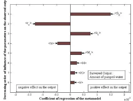
Figures 11, 12 and 13 present the most influential parameters of the developed model while respectively taking the amount of pumped water, the amount of lost water, and the hydram pump efficiency as surveyed model outputs.

Figure 11. Classification of the most dominating factors of the model, pumped water

Figure 12. Classification of the most dominant factors of the model, lost water

Firstly, from section 2.2. Mathematical formulation, 31 parameters are considered in the global sensitivity analysis of the developed model. Then, for both Figures 11, 12, and 13 the parameters on the left are those having a negative effect on the surveyed model output and those on the right have positive effect on this output [40].

As can be seen from Figures 11, 12, and 13 the most influential parameters for the amount of pumped water, for the amount of lost water and for the efficiency of the hydram pump are quite the same, namely:

- the length of the waste valve stroke, S0 - the radius of the waste valve disc, rv - the stiffness of the waste valve spring, k1

- the height of the water column in the delivery pipe, h - the waste valve weight, M1

However, apart from those parameters, if one wants to act specifically on the amount of pumped water it is necessary to consider, firstly, the supply tank height, H and then, the supply pipe radius, r (Figure 11), if the latter goes first for the amount of lost water (Figure 12). On the other hand, if one wants to influence more on the efficiency of the hydram pump, 3 other parameters should be taken into account, namely: the length of the supply pipe from the source to the center of the delivery valve, L1; the length of the supply pipe from the source to the center of the waste valve, L; and the slope of the hydram pump relative to the horizontal, θ (Figure 13).

4. Conclusions

After modelling and the sensitivity analysis of the parameters of the hydraulic ram pump with springs system, the parameters which influence both the amount of pumped water, the amount of lost water and the efficiency of the pump are the same, namely: the length of the waste valve stroke; the radius of the waste valve disc, the stiffness of the waste valve spring, the height of the water column in the delivery pipe, and the waste valve weight.

These results are the same as those of previous studies on the hydraulic ram pump [1, 9, 21]. But if it has been shown that the weight of the waste valve plays an important role on the operation of the pump, this parameter is less important than the stiffness of the waste valve spring in our case.

Therefore, if one wants to have good results for each output independently, it is necessary to act on additional parameters. Those parameters are the same for the amount of pumped and lost water which are: the supply tank height and the supply pipe radius as shown in Figures 11 and 12. For the efficiency of the pump, those parameters are: the length of the supply pipe from the source to the center of the delivery valve, the length of the supply pipe from the source to the center of the waste valve, and the slope of the hydram pump relative to the horizontal as shown in Figure 13.

As for the balloon containing the four springs, it was shown that it has no influence on the operation of the pump.

Indeed, for a classic hydram pump with an air balloon, previous study deduced that compared to the kinetic energy in the supply pipe, the potential energy due to the balloon effect is small and may be neglected [21]. So, as obtained from the global sensitivity analysis of the model, the spring balloon has no effect on the operation of the studied hydram pump. In fact, the balloon is mainly used only to eliminate the noise of the water hammer [17, 41].

The studied spring hydram pump was invented and crafted in Madagascar by Rasetarivelo who applied a patent at the Malagasy Office of Industrial Property (OMAPI) in 2004; the patent is entitled "Pompe à eau à système de ressorts sans autre source d’énergie que l’eau" (hydram pump with springs system without any other source of energy but water), and the application number is 2004/012 [22].

As a follow-up to this study, the techno-economic aspect of the pump could be interesting in case of a small hydropower plant to increase water head. Moreover, a comparison between experimental and simulation results can be carried out too.

Nomenclature

a : velocity of pressure-wave transmission in the supply pipe (m.s-1), given by equation (17) A : cross section of the supply pipe (m2) Av : area of the waste valve (m2)

Ared : cross section of the shrinked pipe (m2)

b : linear head loss coefficient of the supply pipe (-) c : friction coefficient of the waste valve (-), given by

equation (4)

e : thickness of the disk of the waste valve (m) E : modulus of elasticity or Young's modulus of the

supply pipe (N.m-2)

E0 : energy received by the balloon (kg.m), given by equation (37)

E1 : energy lost in the supply pipe and in the delivery valve (kg.m), given by equation (42)

E2 : potential energy due to the compression of the four springs (kg.m), given by equation (44)

E3 : energy of the water directly pumped on the head (h+hd) (kg.m), given by equation (43)

Ev : average stiffness of the waste valve disc (kg.m-1), given by the equation (19)

f : bending of the disk of the waste valve (m), given by equation (20)

F : point charge (N)

F1 : sum of the forces exerted on the waste valve (N), given by equation (7)

g : acceleration of gravity (m.s-2)

h : height of the water column in the delivery pipe (m) h0 : increase of the pressure head necessary to open the

delivery valve (m), given by equation (25) hc : level of water in the balloon (m)

hel : singular head loss by progressive expansion of the pipe (m)

hs : head loss in the supply pipe during the period 3 (m)

hv : singular head loss due to the delivery valve during period 3 (m)

ha : height of the water column necessary to oppose the pressure force of the delivery spring for a full opening (m), given by equation (26)

hred : singular head loss by the progressive reduction of the pipe (m)

hr : the sum of the head losses during period 3 (m), given by (38)

H : height of the supply tank (m)

Hs : static head for closing of the waste valve (m), given by equation (5)

k1 : spring stiffness constant of the waste valve (N.m-1) k2 : spring stiffness constant of the delivery valve

(N.m-1)

k3 : stiffness of each spring in the spring balloon (N.m-1)

ki : sum of the singular head loss coefficients due to obstacles: fitting, elbow and others (-)

ks : coefficient de perte de charge de la conduite d’alimentation (-)

K : modulus of elasticity of water (N.m-2)

kel : head loss coefficient by progressive expansion of the pipe (-), given by equation (41)

kred : head loss coefficient by the progressive reduction of the pipe (-), given by equation (39)

L : length of the supply pipe from the supply tank to the center of the waste valve (m)

L1 : length of the supply pipe from the source to the center of the delivery valve (m)

L2 : length of the delivery pipe (m)

m : friction constant of the delivery valve (m.s-1) M1 : weight of the moving part of the waste valve (kg) M2 : weight of the disc in the balloon (kg)

Mv : equivalent weight of the waste valve (valve + spring) (kg), given by equation (6)

N : number of pushes between period 2 and period 3, given by equation (32)

q : amount of pumped water per cycle (kg.s-1), given by equation (57)

qs : amount of pumped water during the period 3 (kg.cycle-1), given by equation (34)

qsup: quantity of extra pumped water (kg.s-1), given by equation (48)

Q : amount of lost water in a cycle (kg.s-1), given by equation (56)

Q1 : amount of lost water during period 1 (kg.cycle-1), given by equation (14)

Q6 : amount of water lost during the period 6 (kg.s-1), given by equation (54)

r : radius of the supply pipe (m) r2 : radius of the delivery pipe (m) r3 : radius of the shrinked pipe (m)

rb : radius of the disc in the balloon (m) rr: radius of the disc of the delivery valve (m) rv : radius of the disk of the waste valve (m) S0 : length of the waste valve stroke (m) S1 : length of the delivery valve stroke (m) S2 : length of the balloon membrane stoke (m) ti : duration of the period i (i=1 to 6) (s)

tr : the duration of the last push at the end of the period 3 (s), given by equation (30)

T : duration of a complete cycle (s), given by equation (55)

u : thickness of the supply pipe (m)

v0 : value of the water minimum velocity at which the waste valve begins to close (m.s-1), given by equation (3)

vf : velocity of the spring balloon membrane at the end of period 3 (m.s-1), given by equation (46) vi : water velocity in the supply pipe at the end of the

period i (i = 1 to 6) (m.s-1)

vr : velocity of the water in the supply pipe near the end of period 3 (m.s-1), given by equation (31) vB : water velocity at the outlet of the delivery pipe

(m.s-1), given by equation (47) w : water density (kg.m-3)

Greek Letters

α6 : acceleration of the water column in the supply pipe at the end of Period 6 or at the beginning of Period 1 (m.s-2), given by equation (10)

ζ : contraction coefficient (-), given by equation (40) ∆v: reduction in velocity (m.s-1

), given by equation (27)

θ: inclination angle of the pump from the horizontal (°)

θ2 : solid angle in the shrinkage (°)

λ : linear head loss coefficient of the delivery pipe during the pumping of the extra pumped water (-) σ : Poisson’s ratio of the supply pipe material (-) φ : coefficient of drag of the waste valve (-), given by

equation (2)

χ : angle at the enlargement (°)

ψ : factor related to the speed of the pressure-wave transmission, given by equation (18)

REFERENCES

[1] W. M. Lansford and W. G. Dugan, An Analytical and Experimental Study of the Hydraulic Ram. The University of Illinois Urbana, 1941.

[2] Pump handbook, 3rd ed., I. J. Karassik, J. P. Messina, P. Cooper, and C. C. Heald, McGraw-Hill, 2001.

[4] A. H. Gibson, Hydraulics and its Applications. D. Van Nostrand Company New York, 1908.

[5] International Development Research Centre, “Proceeding of a Workshop on Hydraulic Ram Pump (Hydram) Technology”, 1985.

[6] T. D. Jeffery, T. H. Thomas, A. V. Smith, P. B. Glover, and P.D. Fountain, Hydraulic Ram Pumps – A Guide to Ram Pump Water Supply Systems. ITDG Publishing, 1992. [7] D. Jammes and T. Fouant, “Agriculture, Énergie &

Environnement Fiche technique 03 Bélier hydraulique.” Inter-Réseau Agriculture Energie Environnement, p. 5, 2015. [8] H. N. Najm, P. H. Azoury, and M. Piasecki, “Hydraulic Ram Analysis: A New Look at an Old Problem,” Proc. Inst. Mech. Eng., vol. 213, no. 2, pp. 127–141, 1999.

[9] B. W. Young, “Simplified Analysis and Design of the Hydraulic Ram Pump”, Proc. Inst. Mech. Eng., vol. 210, no. 4, pp. 295–303, 1996.

[10] J. Krol, “The Automatic Hydraulic Ram”, Proceedings of the Institution of Mechanical Engineers, vol.165, no.1, pp. 53–73, 1951.

[11] A. Pathak, A. Deo, S. Khune, S. Mehroliya, and M. M. Pawar, “Design of Hydraulic Ram Pump,” Int. J. Innov. Res. Sci. Technol., vol. 2, no. 10, pp. 290–293, 2016.

[12] M. Inthachot, S. Saehaeng, J. F. J. Max, J. Müller, and W. Spreer, “Hydraulic Ram Pumps for Irrigation in Northern Thailand,” Agric. Agric. Sci. Procedia, vol. 5, pp. 107–114, 2015.

[13] A. Deo, A. Pathak, S. Khune, and M. Pawar, “Design Methodology for Hydraulic Ram Pump,” Int. J. Innov. Res. Sci. Eng. Technol., vol. 5, no. 4, pp. 4737–4745, 2016. [14] Ansys CFD-Fluent R14.5, Engineering Simulation and 3D

Design Software. Ansys, Inc.: Canonsburg, Pennsylvania, USA, 2014.

[15] D. F. Maratos, “Technical feasibility of wavepower for seawater desalination using the hydro-ram (Hydram),” Elsevier Sci. B.V., vol. 153, pp. 287–293, 2002.

[16] P. Nambiar, A. Shetty, A. Thatte, S. Lonkar, and V. Jokhi, “Hydraulic Ram Pump: Maximizing Efficiency,” 2015 International Conference on Technologies for Sustainable Development (ICTSD), Mumbai, 2015, pp. 1-4.

[17] L. V Girish, P. Naik, H. S. B. Prakash, and M. R. S. Kumar, “Design and Fabrication of a Water Lifting Device without Electricity and Fuel,” Int. J. Emerg. Technol., vol. 7, no. 2, pp. 112–116, 2016.

[18] S. Sheikh, C. C. Handa, and A. P. Ninawe, “A Generalised Design Approach for Hydraulic Ram Pump: a Review,” Int. J. Eng. Sci. Res., vol. 3, no. 10, pp. 551–554, 2013.

[19] N. S. M. Hussin et al., “Design and Analysis of Hydraulic Ram Water Pumping System,” J. Phys. Conf. Ser. 908 012052, 2017.

[20] ANSYS CFX R15.0, Engineering Simulation and 3D Design Software. Ansys, Inc.: Canonsburg, Pennsylvania, USA, 2015.

[21] J. Krol, “A Critical Survey of the Existing Information Relating to the Automatic Hydraulic Ram,” M.E (Technical

University of Warsaw), 1947.

[22] Rasetarivelo, “Pompe à Eau à Système de Ressorts Sans Autre Source d’Energie que l’Eau”, 2004/012, 2004. [23] S. Sheikh, C. C. Handa, and A. P. Ninawe, “Design

Methodology for Hydraulic Ram Pump (Hydram),” Int. J. Mech. Eng. Rob. Res., vol. 2, no. 4, pp. 170–175, 2013. [24] Riadh Ben Hamouda, Notions De Mécanique des fluides

Cours et Exercices Corrigés Centre de Publication Universitaire Tunis, 2008.

[25] B. Slim, “Chapitre IV : Dynamique des Fluides Réels incompressibles”, in Support de cours Mécanique des fluides, pp.37–46, 2014. [Online]. Available: https://www.technologuepro.com/cours-mecanique-des-fluid es/chapitre-4-dynamique-des-fluides-reels-incompressibles.p df.

[26] E. Abdelkader, Dynamique des Fluides Réels, 2016. [Online]. Available: https://www.researchgate.net/publication/ 315619413_Dynamique_des_fluides_reels.

[27] B. W. Young, “Generic Design of Ram Pumps,” Proc Instn Mech Engrs, vol. 212, no. 2, pp. 117–124, 1998.

[28] J. Twyman, “Wave Speed Calculation for Water Hammer Analysis” Obras y Proy., n. 20, pp. 86–92, 2016.

[29] S. Timoshenko and S. Woinowsky-Krieger, Thoery of Plates and Shells, 2nd ed., McGraw-Hill Book Company, Inc., 1959. [30] P. S. Gujar and K. B. Ladhane, “Bending Analysis of Simply Supported and Clamped Circular Plate,” SSRG Int. J. Civ. Eng., vol. 2, no. 5, pp. 1–7, 2015.

[31] R. Itterbeek, “ Chapitre 10. Compléments de Résistance des Matériaux”, 2016. [Online]. Available:

https ://www.itterbeek.org/fr/index/cours-resistance-materiau x.

[32] M. Pirotton and S. Erpicum, “UE Energie Hydroélectrique : Ecoulements à Surface Libre et Sous-pression.”

[33] H. Guillon, “Hydraulique en Charge”, 2016. [Online]. Available : http://chamilo1.grenet.fr/ujf/main/document/ document.php?cidReq=LPROCSHEGE&id_session=0&gid Req=0&origin=&id=498.

[34] A.-L. Zehour, “Hydraulique Générale”,2016.[Online]. Available: https://www.univ-sba.dz/ft/images/

hydraulique/Hydraulique_Générale.pdf.

[35] J. Vazquez, “Hydraulique Générale”, 2010. [Online]. Available: https://engees.unistra.fr/fileadmin/user_

upload/pdf/shu/COURS_hydraulique_generale_MEPA_201 0.pdf.

[36] M. Agelin-Chaab, “1.11 Fluid Mechanics Aspects of Energy”, in Comprehensive Energy Systems, vol. 1, Elsevier Ltd., pp. 478–520, 2018.

[37] D. Bach, F. Schmich, T. Masselter, and T. Speck, “A review of Selected Pumping Systems in Nature and Engineering - Potential Biomimetic Concepts for Improving Displacement Pumps and Pulsation Damping,” Bioinspiration and Biomimetics, vol. 10, no. 5, pp. 1–28, 2015.

[39] H. Rakotondramiarana, T. Ranaivoarisoa, and D. Morau, “Dynamic Simulation of the Green Roofs Impact on Building Energy Performance, Case Study of Antananarivo, Madagascar,” Buildings, vol. 5, no. 2, pp. 497–520, 2015. [40] H. Rakotondramiarana and A. Andriamamonjy, “Matlab

Automation Algorithm for Performing Global Sensitivity Analysis of Complex System Models with a Derived FAST Method,” J. Comput. Model, vol. 3, no. 3, pp. 17–56, 2013.