A New Planning to Forecasting Fuel Consumption in Iran Transportation Using a Hybrid Algorithm and Artificial Neural Network

(1)

SCITECH

Volume 10, Issue 3

RESEARCH ORGANISATION

March 3, 2018

Journal of Research in Business, Economics and Management

www.scitecresearch.com

A New Planning to Forecasting Fuel Consumption in Iran

Transportation Using a Hybrid Algorithm and Artificial

Neural Network

M.Dehghanbaghi

Department of Industrial Engineering, Faculty of Engineering, Robat Karim Branch, Islamic Azad University, Tehran, Iran

.

Abstract

Forecasting fuel demand is one of the preconditions for energy planning and

management. Fossil fuels, a major part of which is consumed in transportation, are one of the most important energies. Therefore, forecasting fuel demand in transportation is of particular importance. An MLP perceptron neural network has been proposed in this study, which is trained using a Hybrid algorithm. The hybrid algorithm is based on an imperialist competitive algorithm (ICA), in which the specifications of simulated annealing (SA) algorithm have been used. To perform the forecasting, the effective parameters on road transportation including the amounts of ton kilometer of transported goods, person kilometer of passengers, the average age of cargo fleet, and the average age of passenger fleet were identified. The results of the investigation indicate the effective performance of the proposed algorithm in ANN training.

Keywords:

Artificial Neural Network; Hybrid algorithm, Imperialist Competitive Algorithm; Forecasting;

Simulated annealing.

1. Introduction

Given its dual role in the country’s energy supply and foreign exchange income, energy sector is considered as the development infrastructure and has always had a fundamental part in the economic and social sections (Moradi Nasab, Amin-Naseri, Behbahani, & Nakhai Kamal Abadi, 2016; Nasab & Amin-Naseri, 2016) Energy is of great significance with regards to road transportation, which is responsible for 25% of Iran’s energy consumption and is the largest consumer of oil products compared to residential, commercial, industrial, and agricultural sectors. Transportation will result in lots of energy loss if it is not performed by correct and rational planning. Different technical and statistical methods have been developed for forecasting energy consumption and plans in the past few decades yielding various results (Elyasi, Jafarzadeh, & Khoshalhan, 2012; Hasani, Jafarzadeh, & Khoshalhan, 2013; Sojoudi & Saeedi, 2017).

However, no technique or combinations of techniques have been successful enough for forecasting energy demand. On the other hand, neural networks have been widely used for forecasting different types of energy demand. Neural networks have been remarkably successful in energy forecasting (Kazemi, 2011). Some evidences indicate much better performance of neural networks compared with regression based models. The architecture of neural networks for forecasting energy demand has a higher precision in comparison with traditional polynomial methods (Nasr, Badr, & Joun, 2003). Therefore, neural network method has been used in this work for forecasting energy consumption in the road transportation considering its higher accuracy.

(2)

three strategic, tactical and operational levels in planning (Jafarzadeh, Gholami, & Bashirzadeh, 2014; Simchi-Levi, Kaminsky, & Simchi-Levi, 2004). Forecasting energy consumption is done on a monthly basis (tactical level) here. One of the first measures in energy planning is energy forecasting. Energy forecasting has been performed on an yearly basis (strategic level) in all literature reports ((Azadeh, Ghaderi, & Sohrabkhani, 2008; Ekonomou, 2010; Geem, 2011; Joghataie & Dizaji, 2010; Kazemi, 2011; Kermanshahi & Iwamiya, 2002; Limanond, Jomnonkwao, & Srikaew, 2011; Murat & Ceylan, 2006; Nasr et al., 2003; Nizami & Al-Garni, 1995; Sözen & Arcaklioglu, 2007);). Energy forecasting is performed on a monthly basis in this work considering the importance of energy planning in the medium-term (tactical) level and the requirement of energy forecasting.

Here, the artificial neural network are used for energy consumption forecasting. In neural network the aim is to find a set of weights in which the error measure is minimized. Determination of the weights is the optimal problem and the search space is high dimensional and multimodal which is usually polluted by noises and missing data. According to this fact, neural network training needs powerful optimization technique (Askarzadeh & Rezazadeh, 2013; Jafarzadeh, Moradinasab, & Gerami, 2017; Joghataie & Dizaji, 2009; Zeyghami, Bode-Oke, & Dong, 2017, Lashgari, 2017) and metahuristic algorithms are good tools for this purpose.

Eventually, in this paper a Hybrid metaheuristic method has been proposed for training of the proposed neural network algorithm. In order to evaluate the performance of this method, the results obtained using this method have been compared with those of network training using imperialist competitive algorithm (ICA), invasive weed optimization algorithm (IWO) and MATLAB multi-layer perceptron default network. A short review of the prior art follows in section 2. The proposed model including model parameters, multi-layer perceptron network, network training and metaheuristic Hybrid algorithm are explained in details in section 3. The results obtained using the model is finally presented in section 4.

2. Literature Review

Literature survey indicates that artificial neural network (ANN) has been used in different areas; especially energy (Azadeh et al., 2008; Ekonomou, 2010; Geem, 2011; Kalogirou & Bojic, 2000; Kazemi, 2011; Kermanshahi & Iwamiya, 2002; Limanond et al., 2011; Murat & Ceylan, 2006; Nasr et al., 2003; Nizami & Al-Garni, 1995; Sözen & Arcaklioglu, 2007). Some sample forecasting problems are shown here.

Hazim (1989) has developed a computer simulation model for forecasting gasoline and gasoil consumption by public transportation vehicles(Bode-Oke, Zeyghami, & Dong, 2017; Zeyghami & Dong, 2015; Sojoudi, 2017).

Kermanshai and Iwamiya (2002) have developed an artificial neural network for forecasting the peak electrical load in Japan. Two neural networks including three layer back propagation and recurrent neural network have been used in this investigation. Ten parameters were considered as network inputs for forecasting the peak electrical load and the forecasting was ultimately performed using the network by 2020 (Kermanshahi & Iwamiya, 2002).

Nasr et al. (2003) have proposed a neural network model for forecasting gasoline consumption in Lebanon. Four neural network models based on gasoline consumption in the past, gasoline consumption time series and price were proposed in this study. The models were then evaluated based on performance criteria (Nasr et al., 2003).

Morat and Ceylan (2006) proposed a model on the basis of neural network for forecasting energy demand and transportation in Turkey. This model was based on supervised neural network approach and the corresponding economic, social and transportation indexes as inputs. The neural network model in this work is a feedforward model with a propagation training algorithm. The indexes considered in this model included population, growth national product (GNP) and transportation indexes (Murat & Ceylan, 2006).

Sozen and Arcakliglu (2007) have proposed a neural network model for forecasting energy consumption in Turkey.They used three different models for network training in their study. Based on their investigation, neural network model is an appropriate model to estimate the net energy consumption using population and economic indexes (Elyasi et al., 2012; Sözen & Arcaklioglu, 2007).

Azadeh et al. (2008) have proposed a neural network model for forecasting annual electricity consumption in highly consuming Iranian industrial sectors. Such industries as chemical, base metals, inorganic and non-metals are highly energy consuming. It was shown that regression models are not very precise given fluctuations in energy consumption. Thus, a multi-layer perceptron neural network was used for forecasting in this work and ultimately a model based on neural network and ANOVA was developed for forecasting long term electricity consumption in high energy consuming industries (Azadeh et al., 2008).

(3)

Limanound et al. (2011) have used a feedforward neural network model for forecasting energy consumption in the next 20 years in Thailand and forecasted energy consumption during the period of 2010-2030. The various inputs considered in this study were population, number of vehicles and gross national product (Limanond et al., 2011).

Geem et al. (2011) have used a neural network model for forecasting energy consumption in transportation in Korea. The input variables considered in this investigation were net national product, population, petroleum price, number of vehicles and number of trips. Neural network model was selected here as the more efficient method (Geem, 2011).

Kazemi et al. (2011) have used a neural network model for forecasting energy demand based on social and economic indexes. They have used a supervised, multi-layer neural network and BP algorithm for training in this investigation (Abedzadeh, Mazinani, Moradinasab, & Roghanian, 2013; Kazemi, 2011). Abual-Foul (2012)have proposed a model for forecasting energy consumption in one of the Middle Eastern countries based on the annual data. An artificial neural network using four artificial variables including gross national product, population, imports and exports has been used for this purpose (AbuAl-Foul, 2012).

Behrang et al. (2011) proposed the bees algorithm (BA) technique to estimate total energy demand in Iran. Their model estimates energy demand based on population, gross domestic product, import and export data by two forms (exponential and linear) model. They compared the obtained results of BA-DEM models with particle swarm optimization and genetic algorithm demand estimation models to show the accuracy of the BA. Finally their model forecasts energy demand up to year 2030 (Behrang, Assareh, Assari, & Ghanbarzadeh, 2011).

Baskan et al. (2012) proposes a heuristic algorithm based on ant colony optimization for estimating the transport energy demand (TED) based on gross domestic product, population, and vehicle-km. they uses three forms of the improved ant colony for improving estimating capabilities of TED model (Baskan, Haldenbilen, Ceylan, & Ceylan, 2012).

Bastani (2012) has used possible techniques and evaluation models for forecasting production of greenhouse gases and fuel consumption under uncertainty conditions in the USA. This work shows the possible distribution of the emission of greenhouse gases and fuel consumption up to 2050. The parameters, which are the main causes for variations in the production of greenhouse gases and fuel consumption, have been identified and ranked via analysis of uncertainty. The parameters include the kilometers traveled per year and vehicle sales (Bastani, Heywood, & Hope, 2012).

Ozdemir G et al. (2016) developed a hybrid genetic algorithm-simulated annealing (GA-SA) algorithm based on linear regression to forecast natural gas demand of Turkey. They consider gross national product, population, and growth rate as independent variables and forecast the amount of natural gas consumption for years between 2001 and 2009 (Ozdemir, Aydemir, Olgun, & Mulbay, 2016; Zeyghami, Babu, & Dong, 2016, Soltani, 2017) .

3. Proposed Model

In order to make a forecasting model for energy consumption in road transportation in medium term time, the effective parameters must first be identified. The data corresponding to the identified variables have been taken within 84 months (7 years on a monthly basis) and the forecasting model for energy consumption in road transportation has been developed accordingly.

3.1 Model Variables

(4)

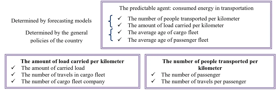
The predictable agent: consumed energy in transportation

 The number of people transported per kilometer

 The amount of load carried per kilometer

 The average age of cargo fleet

 The average age of passenger fleet

which is the energy consumption forecasting and figures B and C show person kilometer of passengers and ton kilometer of goods transported, respectively.

Fig 1: The Factors Forecasted and the Effective Parameters

3.2 Multi-Layer Perceptron Neural Network (MLP)

Multi-layer perceptron neural network is one of the most successful models in forecasting. In general, multi-layer perceptron neural network is composed of an inlet, an outlet and several hidden layers. In neural networks, hidden layer or layers are added to solve resolvable non-linear problems and increase the strength of the network in identification of the algorithms and functions. The number of hidden layers and neurons in each layer of these networks are found by trial and error method; that is, comparison of different network structures in terms of precision of the final model. X = (x1,…,xn) vector is the input signal and z scalar is the output signal of the network. The effect of x on z is determined by w = (w11, w12,…..,wij) vector. The net input to the neuron is shown by net and is defined using the following equation:

Sentence b in this equation is called the bias sentence. Following the entrance of net into the neuron, the actuation function acts with the transfer function, F, to give z output signal via equation z = f(net). The transfer function chosen and used in the hidden layers is a function of hyperbolic tangent, shown in equation 2.

The average root mean square error (RMSE) criterion has been used here to compare the models, as shown in equation 3.

Zm scalar is the output signal of the model and is an actual value.

70% of the data is used for training, 15% is used for testing and the remaining 15% is used for validation. A Hybrid algorithm has been used for network training and the results have been compared with those of other three models.

3.3 Authors Neural Network Training by Hybrid Algorithm

A new algorithm known as hybrid algorithm is presented here based on ICA and SA algorithms. ICA algorithm constitutes the basic structure of this algorithm and the specifications of SA algorithm are used for the displacement of the positions of the colony and imperialist in each decade. The concept of neighborhood in SA algorithm is also used in the proposed algorithm. To define the proposed hybrid algorithm, ICA and SA algorithms are briefly gone over. The proposed algorithm will then be dealt with in details.

3.3.1. Imperialist Competitive Algorithm

Atashpaz-Gargari and Lucas introduced imperialist competitive algorithm (ICA) in 2007. This algorithm is inspired by a social/political process known as imperialist competition. Similar to other evolutionary optimization methods, ICA starts out with a number of initial populations. Each element of the population is called a country in this algorithm. The countries are divided into imperialists and colonies. The best countries (countries with minimum expense of minimization and maximum objective function in maximization problems) are selected as imperialists and other countries form the colonies. Each imperialist conquers and controls a number of non-imperialist countries depending on its power. The power of an imperialist is calculated using an objective function. An imperialist and its colonies make up an empire. The power of an empire is the sum of the imperialist’s power and a percentage of the medium power of its colonies. The colonial policy of assimilation and competition forms the main core of this algorithm. The colonial competition between the early empires starts out such that the colonies of each empire move toward their imperialist and the imperialists also try to increase the number of their colonies. Therefore,

Determined by forecasting models

Determined by thegeneral

policies of the country

The number of people transported per kilometer

 The number of passenger

 The number of travels per passenger

 The number of passenger fleet company

The amount of load carried per kilometer

 The amount of carried load

 The number of travels in cargo fleet

(5)

weaker colonies fall during the competition, ultimately leaving one empire. ICA is applicable in many optimization problems.

3.3.2. SA Algorithm

SA is a local search technique developed by Kirkpatrick. SA approach is a modified version of a local search started with the generation of a primary response. A new response is generated in the vicinity of the existing one in each step (temperature). The new response is accepted if its expense is less than or the same as that of the present response. Otherwise the new response is accepted with a possibility. This possibility depends on the difference between the present and new responses as well as the current temperature. Temperature is a high value moving towards a value near zero. In other words, it decreases periodically as an array. Therefore, wrong responses are accepted in the beginning of SA algorithm and SA moves the responses to reach the best response.

3.3.3. Hybrid Algorithm

The framework of hybrid algorithm is as follows. It must be pointed out that the common parts of this algorithm and ICA algorithm will not be repeated here. This section includes creation of new emperors, movement of colonies towards empires (homogenization), total empire cost, colonial competition and elimination of the weakest empire.

3.3.4. Updating the Colonies of an Empire

A number of neighbors are generated for each empire based on the SA neighborhood definition in this section. In other words, a number of neighbors form in the vicinity of each empire by one of the substitution, succession and reverse policies. The number of neighborhoods for each empire is equal to the number of colonies. Thus, empires with few colonies generate few neighborhoods and vice versa. Following generation of neighborhoods empires, the population of colonies and neighborhoods in the empire merge and the best of them are selected as the number of colonies and are assigned as updated colonies to the corresponding empire.

3.3.5. Revolution

Two situations are selected in each imperialist’s array in each repetition. These situations are substituted with each other and the resulting array then replaces the imperialist’s weakest colony. The process is repeated as a percentage of the total number of situations in each array for each imperialist. This percentage is shown by parameter “Prct-Imp-R”. In addition, some of the colonies are selected and then two situations from the colony’s array are randomly selected and switched. The process is repeated as a percentage of the total number of situations in each array. This percentage is shown by parameter “Prct-Col-R”. A percentage of colonies are selected in each empire for the homogenization process. This percentage is shown by P-R. This process in the ICA algorithm has been reported by (Jafarzadeh, Moradinasab, & Elyasi, 2017; Nazanin Moradinasab, Shafaei, Rabiee, & Ramezani, 2013; Shafaei, Moradinasab, & Rabiee, 2011; Shafaei, Rabiee, & Mazinani, 2012).

3.3.6. Temporary Switching of the Position of Colony and Imperialist

SA algorithm is used for temporary switching of the position of colony and imperialist, as shown below. The best colony of each imperialist ingeneration is selected. The difference between the objective function of each imperialist and the best colony (

 

c

_bestcolony



c

_imperialist) is then calculated. The positions of the imperialist and colony are switched in the minimization problem if



0

. Following the switching, the algorithm is continued with the imperialist in the new position. If



0

, the positions of the imperialist and colony are switched with a probability calculated by

exp(



/

T

)

. T is the control parameter here and is called temperature. Temperature is relatively high in the first generation, but gradually decreases. If

 

0

, the costs of the best imperialist and colony are equal. Therefore, the neighborhoods of the best colonies are constantly checked and the second colony is selected if its cost is not the same as that of the first colony. If the costs are the same, the next colonies are checked.

The selected neighborhood is then used for calculation of





. Given that 0, the positions of the imperialist and colony are switched with a probability calculated by

exp(





/

T

)

. The initial and final temperatures are represented by parameters “To“ and “Tf “, respectively.

3.3.7. World War

(6)

Fig 2: Hybrid Algorithm Pseudocode Algorithm

1. Value Initialization

1.1.Parameters tuning

1.2.Generate the initial countries (randomly in the number of PopSize)

2. Evaluate Fitness Function for each countries

3. Establish the initial Empire (in the number of N-Emp)

3.1.Select the Imperialists

3.2.Align other countries to each Imperialist

4. Assimilate the colonies (in the number of P-Asimlt)

5. Update the colonies

5.1.Generate the neighborhoods for each Imperialist

5.2.Merge the neighborhoods and colonies

5.3.Establish the new colonies

6. Revolution (P-R is the parameter which is shown the percentage of the revolution in each iteration )

7. Calculate

 

c

_bestcolony



c

_imperialist

7.1.If



0

(in minimization)

Exchange the position of the Imperialist and colony

7.2.If



0

Exchange the position of the Imperialist and colony with probability of

exp(



/ )

T

7.3.Else

Calculate





Exchange the position of the Imperialist and given colony with probability of

exp(





/ )

T

8. Calculate

TC

_n



cos (

t imperialist

_n

)





mean

{cos (

t colonies

of empire )}

_n (



is parameter between 0 and 1)

9. Imperialistic competition

10. Eliminate the weak empire

11. World ware

12. Stop if the condition satisfied (the maximum number of the iteration is shown by parameter Max-It

3.4 Numerical Results

A completely connected, multi-layer perceptron neural network with a hidden layer and an output layer has been considered for forecasting energy consumption in the transportation sector. Network inputs include cargo fleet average age, passenger fleet average age, ton kilometer of goods transported and person kilometer of passengers transported. The first two inputs; that is, cargo fleet average age and passenger fleet average age are a function of the country’s policies. However, the ton kilometer of goods transported and person kilometer of passengers transported must be forecasted. Two separate neural networks have been used for forecasting these two inputs.

(7)

Wij= (W11, W12, W21, W22, W13, W23) in the proposed algorithm is shown in Figure 3. The numbers with initial weights are randomly generated.

Fig 3: The Structure of One Response for One Problem With Two Inputs and Three Neurons in the Hidden Layer

W11 W12 W13 W21 W22 W23

-1.2 1.34 1.9 -0.78 -0.97 1.7

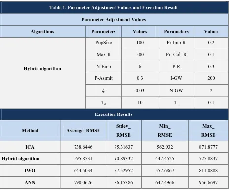
The appropriate adjustment of parameters has been performed for better performance of the proposed algorithm. To do this, the optimal value of each parameter is obtained by varying that parameter while keeping the others constant.

Table 1. Parameter Adjustment Values and Execution Result

Parameter Adjustment Values

Algorithms Parameters Values Parameters Values

Hybrid algorithm

PopSize 100 Pr-Imp-R 0.2

Max-It 500 Pr- Col -R 0.1

N-Emp 6 P-R 0.3

P-Asimlt 0.3 I-GW 200

 0.03 N-GW 2

T0 10 Tf 0.1

Execution Results

Method Average_RMSE Stdev_ RMSE

Min_

RMSE

Max_

RMSE

ICA 738.6446 95.31637 562.932 871.8777

Hybrid algorithm 595.8531 90.89332 447.4525 725.8837

IWO 644.5034 57.52952 557.6867 811.0888

ANN 790.0626 86.15386 647.4966 956.6697

The optimal values of the parameters for experimental simulation were determined after several simulations. Having adjusted the parameters, the problem is solved using a neural network with the proposed hybrid algorithm and three other algorithms including ICA, IWO and the default neural network MATLAB R2012b. All four neural networks are executed 20 times in Matlab R2012b modeling software. The results of the execution are shown in Table 1. The results are evaluated on the basis of the root mean square error of validation measurement criterion.

(8)

The best weights are selected for forecasting from the executions of the two layer perceptron neural network with four neurons in the hidden layer using hybrid algorithm training method.

As previously indicated, in order to forecast the energy consumption, four parameters including ton kilometer of goods transported, person kilometer of passengers transported, cargo fleet average age, and passenger fleet average age are used. Therefore, the main network, which is forecasting energy consumption, must be modelled by the two layer perceptron neural network using hybrid algorithm training method. The corresponding data for the network are the monthly data, which are categorized into training (70%), test (15%) and validation data (15%) groups. The input data for each year are used for forecasting energy consumption during the same year. Thus, the first step in this investigation is the determination of ton kilometer of goods transported, person kilometer of passengers transported, cargo fleet average age, and passenger fleet average age. Therefore, the neural network trained using the hybrid algorithm is used for forecasting ton kilometer of goods transported. The three inputs of this network are the number of fleet companies, the number of fleets and the quantity of fleet transported.

Monthly data for 2000-2005 periods have been used for forecasting the ton kilometer of goods transported. The default data are randomly categorized into training (70%), test (15%) and validation data (15%) groups. Since it is desirable to design a network, which can forecast the ton kilometer of goods transported in the next three years using the data from a given month, the outputs for each month are placed for the inputs of the same month for the next three years for network design.

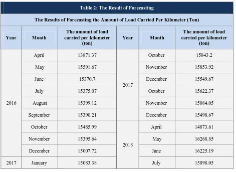
For example, the output data for April of 2002 are placed for the inputs for April of 2000. Ultimately, using the inputs for the months of 2000, the ton kilometer of goods transported in the year 2002 are forecasted and thus the ton kilometer of goods transported during 2015 are forecasted using the data for 2012. Given that the objective of this research is forecasting energy consumption in the 2016-2018 period (36 months), the data for 2000-2012 period are used for forecasting 2016-2018 period after network training. The MLP perceptron neural network is now ready for forecasting the ton kilometer of goods transported. Thus, the monthly input data for the years 2013-2015 can be used for forecasting the ton kilometer of goods transported during the months of 2016-2018 period. The results of forecasting the ton kilometer of goods transported are shown in Table 2.

Afterwards, the person kilometer of passengers transported is forecasted by the two layer perceptron neural network and the data during the years 2000-2012 using hybrid algorithm, similarly to forecasting the ton kilometer of goods transported. The forecasting results for the months of 2016-2018 range are shown in Table 2.

Table 2: The Result of Forecasting

The Results of Forecasting the Amount of Load Carried Per Kilometer (Ton)

Year Month

The amount of load carried per kilometer

(ton)

Year Month

The amount of load carried per kilometer

(ton)

2016

April 13871.37

2017

October 15843.2

May 15591.67 November 15853.92

June 15370.7 December 15549.67

July 15375.07 October 15622.37

August 15399.12 November 15084.05

September 15390.21 December 15498.67

October 15485.99

2018

April 14873.61

November 15395.64 May 16268.85

December 15007.72 June 16225.19

(9)

February 15087.36 August 15889.14

March 19806.83 September 15883.13

April 14675.83 October 15903.49

May 15939.13 November 15531.74

June 15952.99 December 15475.74

July 15648.49 October 15782.95

The results of forecasting the person kilometer of passengers transported

Year Month

The number of people transported

per kilometer

Year Month

The number of people transported per

kilometer

2016

April 4495.503

2017

October 4832.105

May 4204.293 November 4785.323

June 4501.736 December 5028.667

July 4369.164 October 5904.295

October 4329.899

2018

April 5217.959

November 4455.429 May 4383.322

December 4595.622 June 4570.192

2017

January 5394.419 July 4617.474

February 5210.174 August 5918.428

March 4749.69 September 4736.524

April 4931.868 October 4854.126

May 4426.547 November 4861.048

June 4731.511 December 5231.926

July 5123.52 October 5101.036

(10)

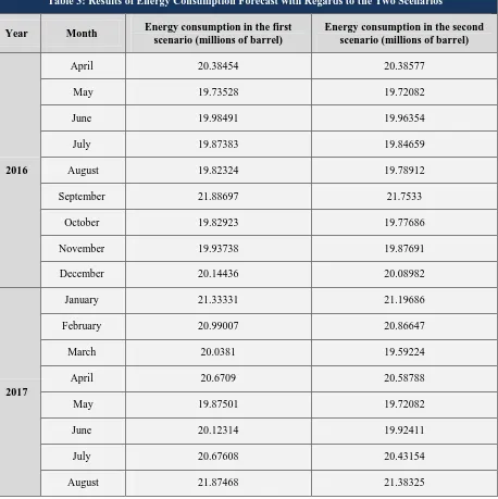
In order to forecast energy consumption in the transportation sector on a monthly basis in the 2016-2018 range, two parameters, namely ton kilometer of goods transported and person kilometer of passengers transported were forecasted during the months of 2016-2018 range. The other two parameters; that is, cargo fleet and passenger fleet average age were functions of the government policy. Therefore, with regards to the government policies, two possible scenarios for forecasting these parameters are considered.

A: Scenario 1:

With regards to cargo fleet and passenger fleet average age, the government will not take add new fleet to the system or renovate the aging fleet. Thus, the fleet average age (cargo or passenger) will be calculated in the range of 2016-2018, without the addition of new fleet. The energy consumption in the transportation sector will then be forecasted by two layer perceptron neural network using hybrid algorithm training.

B:Scenario 2:

During its objectives in the fourth and fifth economic development plan in the transportation sector, which is achieving an average age of 10 years in both cargo and passenger fleets, the government will carry out renovation of the aging fleet. The energy consumption in the transportation sector in the 2016-2018 periods will then be forecasted by two layer perceptron neural network using hybrid algorithm training considering the new data.

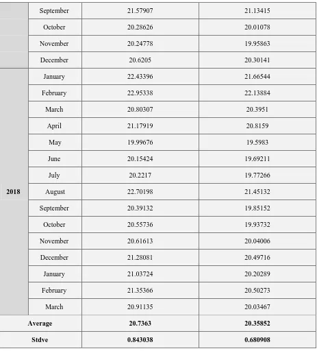
Table 3: Results of Energy Consumption Forecast with Regards to the Two Scenarios

Year Month Energy consumption in the first scenario (millions of barrel)

Energy consumption in the second scenario (millions of barrel)

2016

April 20.38454 20.38577

May 19.73528 19.72082

June 19.98491 19.96354

July 19.87383 19.84659

August 19.82324 19.78912

September 21.88697 21.7533

October 19.82923 19.77686

November 19.93738 19.87691

December 20.14436 20.08982

2017

January 21.33331 21.19686

February 20.99007 20.86647

March 20.0381 19.59224

April 20.6709 20.58788

May 19.87501 19.72082

June 20.12314 19.92411

July 20.67608 20.43154

(11)

September 21.57907 21.13415

October 20.28626 20.01078

November 20.24778 19.95863

December 20.6205 20.30141

2018

January 22.43396 21.66544

February 22.95338 22.13884

March 20.80307 20.3951

April 21.17919 20.8159

May 19.99676 19.5983

June 20.15424 19.69211

July 20.2217 19.77266

August 22.70198 21.45132

September 20.39132 19.85152

October 20.55736 19.93732

November 20.61613 20.04006

December 21.28081 20.49716

January 21.03724 20.20289

February 21.35366 20.50273

March 20.91135 20.03467

Average 20.7363 20.35852

Stdve 0.843038 0.680908

Table 3 shows the results of energy consumption forecast with regards to both scenarios. The results indicate that energy consumption will decrease considerably by carrying out the renovation plan.

3.5 Conclusion

(12)

the model indicate reduction of energy consumption in the case of renovating of the fleet. Further research may be carried out concerning the evaluation and forecasting the whole country’s energy consumption and/or using new metaheuristic methods or a combination of them for network training.

References

[1]

Abedzadeh, M., Mazinani, M., Moradinasab, N., & Roghanian, E. (2013). Parallel variable

neighborhood search for solving fuzzy multi-objective dynamic facility layout problem. The

International Journal of Advanced Manufacturing Technology, 65(1-4), 197-211.

[2]

AbuAl-Foul, B. M. (2012). Forecasting Energy Demand in Jordan Using Artificial Neural

Networks. Topics in Middle Eastern and African Economies, 14.

[3]

Askarzadeh, A., & Rezazadeh, A. (2013). Artificial neural network training using a new efficient

optimization algorithm. Applied Soft Computing, 13(2), 1206-1213.

[4]

Azadeh, A., Ghaderi, S., & Sohrabkhani, S. (2008). Annual electricity consumption forecasting by

neural network in high energy consuming industrial sectors. Energy conversion and

management, 49(8), 2272-2278.

[5]

Baskan, O., Haldenbilen, S., Ceylan, H., & Ceylan, H. (2012). Estimating transport energy demand

using ant colony optimization. Energy Sources, Part B: Economics, Planning, and Policy, 7(2),

188-199.

[6]

Bastani, P., Heywood, J. B., & Hope, C. (2012). US CAFE Standards: Potential for Meeting

Light-Duty Vehicle Fuel Economy Targets, 2016–2025. Massachusetts Institute of Technology,

Cambridge, Massachusetts.

[7]

Behrang, M., Assareh, E., Assari, M., & Ghanbarzadeh, A. (2011). Total energy demand

estimation in Iran using bees algorithm. Energy Sources, Part B: Economics, Planning, and

Policy, 6(3), 294-303.

[8]

Bode-Oke, A. T., Zeyghami, S., & Dong, H. (2017). Optimized Body Deformation in Dragonfly

Maneuvers. arXiv preprint arXiv:1707.07704.

[9]

Ekonomou, L. (2010). Greek long-term energy consumption prediction using artificial neural

networks. Energy, 35(2), 512-517.

[10]

Elyasi, M., Jafarzadeh, H., & Khoshalhan, F. (2012). An economical order quantity model for

items with imperfect quality: A non-cooperative dynamic game theoretical model. Paper

presented at the 3rd International Logistics and Supply chain Conference.

[11]

Geem, Z. W. (2011). Transport energy demand modeling of South Korea using artificial neural

network. Energy Policy, 39(8), 4644-4650.

[12]

Hasani, R., Jafarzadeh, H., & Khoshalhan, F. (2013). A new method for supply chain coordination

with credit option contract and customers’ backordered demand. Uncertain Supply Chain

Management, 1(4), 207-218.

[13]

Jafarzadeh, H., Gholami, S., & Bashirzadeh, R. (2014). A new effective algorithm for on-line

robot motion planning. Decision Science Letters, 3(1), 121-130.

[14]

Jafarzadeh, H., Moradinasab, N., & Elyasi, M. (2017). An Enhanced Genetic Algorithm for the

Generalized Traveling Salesman Problem. Engineering, Technology & Applied Science Research,

7(6), 2260-2265.

(13)

[16]

Joghataie, A., & Dizaji, M. S. (2009). Nonlinear analysis of concrete gravity dams by neural

networks. Paper presented at the Proceedings of the World Congress on Engineering.

[17]

Joghataie, A., & Dizaji, M. S. (2010). Transforming results from model to prototype of concrete

gravity dams using neural networks. Journal of Engineering Mechanics, 137(7), 484-496.

[18]

Kalogirou, S. A., & Bojic, M. (2000). Artificial neural networks for the prediction of the energy

consumption of a passive solar building. Energy, 25(5), 479-491.

[19]

Kazemi, A., Shakouri, H., Menhaj, M.B., Mehregan, M.R., and Neshat, N. (2011). Commercial

Energy Demand Forecast: Iran Case Study. 3rd International Conference on Information and

Financial Engineering.

[20]

Kermanshahi, B., & Iwamiya, H. (2002). Up to year 2020 load forecasting using neural nets.

International Journal of Electrical Power & Energy Systems, 24(9), 789-797.

[21]

Lashgari Y. (2017). Proposing a hierarchical approach based on fuzzy logic to choose a

contractor in the bank. International Academic Journal of Science and Engineering, 4(3), 28-38.

[22]

Limanond, T., Jomnonkwao, S., & Srikaew, A. (2011). Projection of future transport energy

demand of Thailand. Energy Policy, 39(5), 2754-2763.

[23]

Moradi Nasab, N., Amin-Naseri, M., Behbahani, T. J., & Nakhai Kamal Abadi, I. (2016). An

integrated economic model of fossil fuel energy planning for government and private sectors.

Energy Sources, Part B: Economics, Planning, and Policy, 11(7), 651-664.

[24]

Moradinasab, N., Shafaei, R., Rabiee, M., & Ramezani, P. (2013). No-wait two stage hybrid flow

shop scheduling with genetic and adaptive imperialist competitive algorithms. Journal of

Experimental & Theoretical Artificial Intelligence, 25(2), 207-225.

[25]

Murat, Y. S., & Ceylan, H. (2006). Use of artificial neural networks for transport energy demand

modeling. Energy Policy, 34(17), 3165-3172.

[26]

Nasab, N. M., & Amin-Naseri, M. (2016). Designing an integrated model for a multi-period,

multi-echelon and multi-product petroleum supply chain. Energy, 114, 708-733.

[27]

Nasr, G., Badr, E., & Joun, C. (2003). Backpropagation neural networks for modeling gasoline

consumption. Energy conversion and management, 44(6), 893-905.

[28]

Nizami, S. J., & Al-Garni, A. Z. (1995). Forecasting electric energy consumption using neural

networks. Energy Policy, 23(12), 1097-1104.

[29]

Ozdemir, G., Aydemir, E., Olgun, M. O., & Mulbay, Z. (2016). Forecasting of Turkey natural gas

demand using a hybrid algorithm. Energy Sources, Part B: Economics, Planning, and Policy,

11(4), 295-302.

[30]

Shafaei, R., Moradinasab, N., & Rabiee, M. (2011). Efficient meta heuristic algorithms to

minimize mean flow time in no-wait two stage flow shops with parallel and identical machines.

International Journal of Management Science and Engineering Management, 6(6), 421-430.

[31]

Shafaei, R., Rabiee, M., & Mazinani, M. (2012). Minimization of maximum tardiness in a no-wait

two stage flexible flow shop. International Journal of Artificial Intelligence™, 8(S12), 166-181.

[32]

Simchi-Levi, D., Kaminsky, P., & Simchi-Levi, E. (2004). Managing the supply chain: the definitive

guide for the business professional: McGraw-Hill Companies.

[33]

Soltani, R. (2017). Modeling integrated flow shop Scheduling problem and air transportation in

supply chain. International Academic Journal of Science and Engineering, 4(3), 10-19.

(14)