Short RCC Column Performances in Different Conditions: Axial, Uniaxial & Biaxial Bending

Short RCC Column Performances in Different Conditions:

Axial, Uniaxial & Biaxial Bending

A. B. M. Golam Rabbany1_{, Samiul Islam}2_{, Md. Hasan-Uz-Zaman}3

1_{Civil Engineering Department, Tung Hing (BD) MFY Ltd, Comilla, Bangladesh} 2_{Structural Engineering Department, Hifab International AB, Dhaka, Bangladesh}

3_{Engineering Department, Northern Techno Trade, 20 Escaton Garden, Escaton, Dhaka, Bangladesh}

Abstract

bending moment also. Most of the columns are designed as short columns in practice. But in practical cases we cannot use short column in all situations. Short columns can be designed by first order analysis. Balanced failure concept is an essential and important step to design a short column. It gives an idea to the designer about how much load (Both axial & bending) a column can carry safely. During design work the column load / column position may be changed for some reasons (Architectural purpose or client requirements or accidentally). With the change of column load / column position; column forces or moments are changed. Again with the change of column orientation neutral axis is also changed with a significant amount which affects the other values such as load, moment carrying capacity etc. For uniaxial bending column balanced failure concept is an important step. But actual neutral axis calculation is a matter of study. Different approach gives different values and different column section has different neutral axis distance. Without getting proper neutral axis distance load, moment & corresponding eccentricity cannot be accurate. In this study the changing pattern / behavior of column load/moment/location would be studied which may help the designer to predict the column performances in different conditions. In this study, some guideline is followed as per CRSI handbook 2008, ACI code and some other reliable resources. Axial load, axial with eccentric load and biaxial bending are considered and different types of column is compared to decide the safe and optimum steel and section dimension in column design.

Keywords

1. Introduction

1.1. Background of This Study

Column is the main part of a structure. A beam failure would normally affect only a local region, whereas a column failure could result in the collapse of the entire structure. During design work the column load or orientation may be changed for some reasons (Architectural purpose or client requirements). With the change of column load; stresses in steel in tension and compression zone also changed. It’s necessary for a structural engineer to know the internal stresses in different parts of column which may help to decide which side of column experiences more stress and need more steel. If the column is axially loaded then the steel bar provided in any pattern no matter. But if the column is in uniaxial bending it needs to place the steel bar in the two

* Corresponding author:

palashruet@gmail.com (A. B. M. Golam Rabbany) Published online at http://journal.sapub.org/jce

Copyright©2018The Author(s).PublishedbyScientific&AcademicPublishing This work is licensed under the Creative Commons Attribution International License (CC BY). http://creativecommons.org/licenses/by/4.0/

faces parallel to the axis of bending (strong axis). In case of biaxial bending we need to place the steel bar all the four faces.

This study helps a structural engineer to select the proper steel ratio and pattern of steel placing position and column performances for different material properties and different loading conditions. In his study only short tied column will be discussed.

1.2. Short Column

Shortly, If the ratio of the lowest dimension of a column and effective length of column is less than or equals to 12 then the column is considered as short column.

1.3. Different Types of Column in Practical Cases

In the above plan C1 is considered as axial column as the spacing in X and Y direction is equal.

The C2 and C3 is uniaxial & biaxial bending column respectively.

The C1 also may be considered as uniaxial or C2 may be biaxial column if the span related to it is not equal.

Figure 1. Different types of column depend on position [1]

2. Axial Loaded Column

2.1. Introduction to Axial Loaded Column

Generally it’s not possible to construct a column which is 100% axially loaded. For construction process we cannot avoid some error in some cases. For particular it may be possible to ensure perfect straight when building a 2 story building. But in case of 5 stories we cannot make straight up. However there is a guideline to assume the loading as axial in case of small eccentricity. If the load is within the eccentricity 5% of the lateral dimension of column is considered as an axially loaded column (Zero /Negligible moment).

Previously in ACI code some eccentricity is considered based on e/h ratios but the updated code omits this provision and recommends using an overall reduction factor in case of any accidental eccentricity as 0.80. [2]

2.2. Design Load Calculation Procedure

The rate of loading in most of the structure is slower than in a cylinder test. During construction work the concrete have some voids in it and some fault during workmanship.

So we cannot use or get the full value of concrete compressive stress which is obtained from cylinder test.

Test have shown that the maximum reliable compressive strength of reinforced concrete is about 0.85f’c.

The calculation of axial load carrying capacity is based on the following formula

P= (0.85f’cAg) + (Ast fy) (1) In the above equation,

Load carried by concrete=0.85f’cAg Load carried by steel= Ast fy f’c = concrete compressive strength fy = Steel yield strength

Ag= Gross concrete area of column Ast = steel area

For tied column we need to multiply P with 0.65and 0.70 for spiral column. This reduction factor is called as building importance factor. (Spiral column is not considered in this study).

Column may experience some eccentricity and for this reason we may further multiplied the P with another reduction factor 0.80.

The steel occupy some concrete area which is very low (which is equal to the steel ratio). So it’s not considered in the above equation (1). From calculation it’s shown that it deviates the column load by less than 1%.

2.3. Column Capacity Depending on Material Properties

The equation used to calculate load capacity of axial column is linear (Equation 1). So if we use high strength concrete or high grade steel; the load increased as the same percentage of the corresponding increase of the materials.

2.4. Reinforcement Ratio

Generally 0.01 to 0.08 reinforcement ratio is used for RCC column [3]. But in actual practice maximum steel ratio 0.04 is used in most of the cases because in case of bar lapping if 50% steel bar lap in one place then automatically the reinforcement ratio increased 1.5 times. It should be consider when selecting steel ratio.

3.

Axial Load & Uniaxial Bending

3.1. Load with Moment about one Axis

In this type of column at first we need to have a look in the balanced failure point which is defined as the point where the steel in both zone (Tension & compression) yields.

From this limiting value we can get an idea about how much maximum axial force and bending force the column could carry with the corresponding eccentricity.

3.2. Balanced Failure Concept

Figure 2. (a) Column with axial load and bending (b) Equivalent load P with eccentricity e (c) Loaded column

(d) Strain distribution (e) Stresses & forces

For every column of this type has a couple of P & M at which balanced failure occurs.

If e= 0, then the column is a pure axial column (P=Po) If the columns have some moments then we can calculate the corresponding e for different values of M & P.

If we plot all the e, p & M in a graph, then we can get a diagram (Qualitative) as like as Figure 3 which is named as Column interaction diagram.

Figure 3. Column interaction diagram (Qualitative)

From the Figure 3 we can see a point eb where the compression steel and tension steel both yield.

The green portion above the eb represents the compression failure region and the grey portion is the tension failure region.

3.3. Balanced Load (Pb), Balanced Moment (Mb) & Balanced Eccentricity (eb) Calculation

For balanced failure case at first we need to draw a strain diagram for the column section we discussed.

Figure 4. Strain diagram of column Section (Typical) [3]

3.3.1. Case 1 (Trial Section 300 mm X 300 mm)

Cb=Neutral axis distance (from the heavily loaded side) of the column

d’= Compression zone steel bar centroid from face d= Tension zone steel bar centroid from face fs=Stress in tension steel

f’s= Stress in compression steel εu=Concrete Strain

fy= 415 MPa (60 ksi) f'c= 27.5MPa (4 ksi)

Es= 200 GPa (Modulus of Elasticity of steel) Concrete Strain, εu =0.003

(At balanced failure, concrete reaches its maximum strain and it is 0.003).

Steel strain,

εy =fy/Es=0.0021

d & d' depend on the bar dia and clear cover. In this case clear cover 38 mm (1.5") and using 16 mm dia bar.

At balanced failure point,

f's= 0.003*200*103_{*(Cb-d')/Cb (2)}

which is less than or equals to fy

fs= 0.003*200*103_{*(d-Cb)/Cb (3)}

which must be less than or equals to fy

a= 0.85*Cb

C=Concrete compressive resultant (0.85f”c ab) 3.3.2. Result Analysis for 300 mm X 300 mm Section

6#16mm bar, b=300 mm, h=300 mm (Using Figure 4) (Table 1 in Appendix A)

Cb= 149.4 mm, f's and fs are 415.26MPa and 420 MPa respectively; as per the conventional method equation (4).

But the maximum value is 415 MPa which cannot be exceeded. That means this value have some errors. In the equation (2) & (3), the only two variables we have unknown Cb & f’s or fs. Cb is considered as an imaginary distance of the neutral axis from the heavily loaded side.

The d' & d are fixed. That means the error is in the value of Cb.

We can eliminate the error or calculate the error in different ways. At first we may put f's=415 MPa in the equation (2) and then we get a value of Cb and confirm that the fs is how much. Secondly, we may put fs=415 MPa in the equation (3) and then we get a value of Cb and confirm that the f's is how much.

3.3.3. Comparison Study

(Value of Cb calculated from different approach in Table 1 in Appendix A)

Table 3.1 Calculation method to obtain

neutral axis Cb,mm C,KN e,mm Conventional approach in

equation (4) 149.4 894 144.7 By putting f's=415 MPa in

equation (2) 153.3 917 141.6 By putting fs=415 MPa in

equation (3) 149.4 894 144.7

Figure 5. Interaction diagram for case 1

For 300mm X 300mm section we found that the conventional method and another two methods give the same value of Cb (Negligible discrepancy). From the above analysis we again found that the balanced failure point is not

a single point which is denoted by eccentricity eb.

For calculation easiness, we consider/imagine eb is a single point but it actually a range in some cases.

From Table 1 in Appendix A, we can see that if the load is 144.7 mm distance from the center point of the column both (tension & compression steel yield).

Again, if the load is 141.60 distance from the center point of the column then compression steel yield before the tension steel yield. This calculation is also done by using balanced failure formula.

That means the balanced eccentricity is written as eb= 141.6 mm to 144.7mm.

The balanced load Pb = 894~917.

For comparison we again try to calculate the Cb for the section with unequal b & h.

3.3.4. Case 2

Balanced Failure Concept (Trial Section 500 mm X 300 mm):

Material properties and equation are same as like as case 1 except the column section.

d & d' depend on the bar dia. The following values of d & d' are for clear cover 47.5 mm and using 20 mm dia bar for

500 mm X 300 mm section. b=300mm & h=500mm.

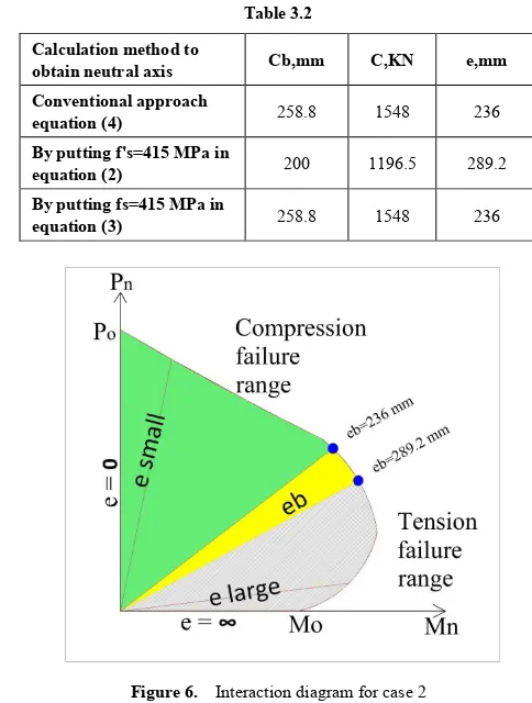
Table 3.2 Calculation method to

obtain neutral axis Cb,mm C,KN e,mm Conventional approach

equation (4) 258.8 1548 236 By putting f's=415 MPa in

equation (2) 200 1196.5 289.2 By putting fs=415 MPa in

equation (3) 258.8 1548 236

Figure 6. Interaction diagram for case 2

3.3.5. Result Analysis for 500 mm X 300 mm Section 6#20 mm bar, b=300mm, h=500mm (Using Figure 4)

(Table 2 in Appendix A)

(Actually the calculation shows f’s and fs more than 415 N/mm22_{. We use Fe415 in this case, so value of f’s and fs can}

be possible to exceed this value. The cause is described in 3.3.2).

For confirmation we can try again by using the before two procedures to calculate Cb by putting f's=415 MPa in equation 2 & fs=415 MPa in equation 3. In the previous trial section 300mm X 300mm the result is quite same but in this case the eccentricity is so far different from different approach.

From Table 2 in Appendix A, we can see that if the load is 236mm distance from the center point of the column both (tension & compression steel yield).

Again, if the load is 289.2 distance from the center point of the column both (tension & compression steel yield).

That means the balanced eccentricity is written as eb= 236 mm ~ 289.2 mm (More than 5% deviation). In case of comparison study we know any change more than 5% should be considered and significant.

The balanced load Pb = 1196~1548 (more than 20% deviation).

As per CRSI handbook the balanced failure for 100% fy stress (For balanced failure point) the design balanced load is 1014 KN (With reduction factor 0.65) [4].

3.3.6. Case 3

Balanced Failure Concept (For trial Section 300mm X 500 mm)

All properties same as Case 2 The only difference is h=300mm & b = 500 mm.

Table 3.3 Calculation method to obtain

neutral axis Cb,mm C,KN e,mm Conventional approach

equation (4) 141.2 1407.6 140 By putting f's=415 MPa in

equation (2) 200 1994 100.3 By putting fs=415 MPa in

equation (3) 141.2 1407 140

Figure 7. Interaction diagram for case 3

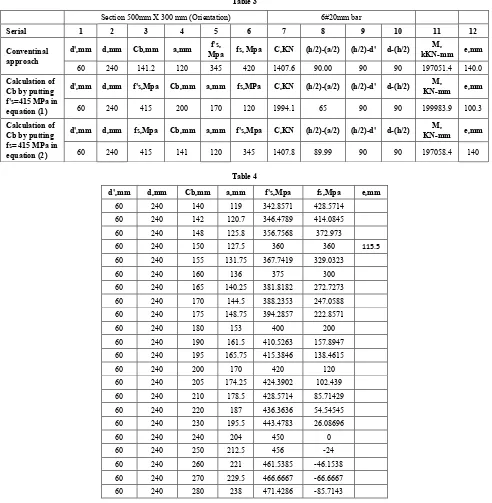
For case 3 we cannot get any point where the two steel (Compression & tension steel) yields at the same couple of P & M. Detail’s calculations are provided in Table 3 in Appendix A.

3.3.7. Result Analysis for 300mm X 500 mm From conventional method we get

Cb = 141.2 mm where fs=420 MPa but f’s=345 MPa By putting f's=415 MPa, Cb = 200mm but fs= 120 MPa By putting fs=415 MPa, Cb = 141.2mm and f’s= 415 MPa By trial calculation we get that when Cb=150 mm, then tension & compression steel reaches at their balanced condition but the value of f's=fs=360 MPa.

The corresponding eccentricity is e=115 mm (From Table 4 in Appendix A). Neutral axis changes with the change of orientation of column its ok. But for this change we also get different values of P & M.

We must make an imagination by experience that to select the strong axis.

Usually the strong axis is the axis which is perpendicular to h. (where h>b) From the neutral axis calculation sometimes we need calculate the Case 3 (Same column section but different orientation) because from experience the large moment is about the strong axis and associated with large load. For safety we need to reconfirm the neutral axis value for different orientation of column section. It ensures any kinds of accidental eccentricity in case of tall building or special structure (Watch tower, hanging bridge, water tank, cantilever structure etc.)

In case of 300mm X 300mm the b and h are same but for

300mm X 500 mm we have two options to assume b & h. From pile cap design it is seen that in case of deep beam conventional beam method is not applicable or not efficient. [5]. Similarly conventional method does not give proper neutral axis value in all column section. We cannot find balanced neutral axis value in case of 300mm X 500 mm

section when we use h=300mm and b=500 mm.

However, generally the neutral axis is calculated from the heavily loaded side of a column section. Because the other side also may have some forces (axial/bending) which may cause excessive stress in some portion. From the Table 2 we get Cb from 500 mm X 300 mm section But for 300mm X 500 mm we cannot get any point where the both steel (Tension & compression ) yields.

From the above calculation we can see that we cannot get balanced failure point in all cases.

It depends on the value of b and h and also depends on the selection of b & h.

b & h are dependent of axis selection which axis is considered as strong axis and weak axis.

Most of the cases in balance failure condition by conventional method fy= 415 MPa.

3.3.8. Steel Placement to Get Ultimate Benefit

In the moment equation using the (Figure 2 (b)(c)(d)). we get

M = P {(h/2)-(a/2)} + Ast*fy*{(h/2)-(d')}

+A’st{(d-(h/2)} [6] (5) We can achieve desired moment carrying capacity by increasing Ast, A'st or Ag. Sometimes we cannot increase concrete area of column due to architectural bindings.

In that case we need to increase steel percentage but placing the steel bar in proper position is also a matter of study.

Figure 8. Steel strain and stress depending on position

From the above section 300mm X 500 mm we can see that Y-Y' is the strong axis. That means we need to place the column in the gridline in that orientation if the maximum moment is about Y-Y' axis. Similarly most of the steel bar should be placed parallel to the Y-Y' axis. From calculation of stress we can see that the neutral axis is 158.88 mm.

When large bending moments are present it is most economical to concentrate all or most of the steel parallel to the axis of bending.

From the calculation in Table 3.4 the steel in Y-Y axis carry a few amount of load and ultimately carry a few amount of moment. This steel has a significant contribution in case of axial load carrying capacity rather than moment. We may also calculate the neutral axis as like as section 3.3 where the column base b=300mm and h=500 mm which give us a proper value that steel has how important or not in case of bending moment about X-X' axis. In this case the steel bar in grid line 3-Y, 4-Y have less strain as compared to the strain in the steel in grid line 1-1 & 2-2.

3.3.9. Some Example of Changing of Neutral Axis Position Sometimes due to construction mistake we need to recalculate the neutral axis position.

In the picture the clear cover of the steel is deviated from the actual position. To avoid any problem its need to recalculate the neutral axis position and corresponding column capacity in this case whatever it complies with the main drawing and the onsite position.

Figure 9. The clear cover is deviated due to poor workmanship and for this reason neutral axis location will be changed which must be considered in case of revised design [7]

Table 3.4

Concrete strain is 0.003 Corresponding strain _{from similar triangle} Corresponding _{stress, MPa} Steel _area Load contribution _(KN)

The strain in steel in grid 1 0.00225 450 942 390.9 The strain in steel in grid Y-Y' 0.000102 20.4 942 19.2

The strain in steel in grid 2 0.0023 460 628 288.9

4.

Biaxial Bending

4.1. Introduction to Biaxial Bending Column

In this type of column the load is in a position which is

some distance from X axis as well as from Y axis.

Generally reciprocal method & load contour method is used to design this type of column.

the most severe loading condition, an equivalent uniaxial moment can be used for the preliminary selection of a cross section shape and for longitudinal reinforcement. [8]

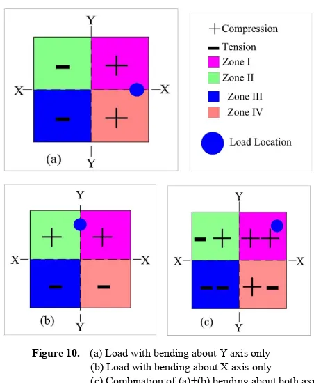
Figure 10. (a) Load with bending about Y axis only (b) Load with bending about X axis only

(c) Combination of (a)+(b) bending about both axis

From the section 3 we get an idea about uniaxial bending. We also get a balanced eccentricity at which steel in compression and tension zone both yields.

For biaxial bending,

In the above picture we can see that when the load is on the X axis it causes tension in the zone II & III and compression in the Zone I & IV.

Again if the load on the Y axis it causes tension in the zone III & IV and compression in the Zone I & II.

4.2. Reciprocal Load Method

According to Bresler’s method [9] the value of nominal load in biaxial column is

1/Pn = (1/Pno)+(1/Pnyo)+(1/P) (7)

Figure 11. Biaxial bending column (Section 500mm X 300mm)

Pn = Approximate value of nominal load in biaxial bending with eccentricities ex (Distance from Y axis) and ey (Distance from X axis)

Pnyo = Nominal load when ex is present (ey=0) Pnxo = Nominal load when ey is present (ex=0) Po = Nominal load for concentrically loaded column Pnyo, Pnxo and Po is calculated from Graph [10] (A.5, A.6, A.7) using the values γ, ex/h & Ast/bh.

4.3. Example Calculation

Trial Section 500mm X 300mm

In the Figure 10 the load is located at a distance ex from Y axis and ey from the X axis.

dx= c/c distance of steel bar(Outer to outer bar) in X direction=380 mm

dy= c/c distance of steel bar (Outer to outer bar)in X direction=180 mm

Ast=Area of steel=8#9 bar=8*490.88=3927 sq.mm

Table 4.1. Balanced Load in different location (Associated with Figure 12)

Load Location ex ey P Load type 1 0 0 5148 Axial

2 290 0 1548 Uniaxial

3 290 290 773 Biaxial

4 145 0 3095 Uniaxial

5 145 145 1139 Biaxial

6 72 72 2167 Biaxial

7 36 36 3773 Biaxial

Figure 12. Different values of load for different location (Section 500mm X 300mm) as per above table

Step 1 (Considering Bending about Y axis) γ = dx/h=380/500=0.76~0.75

ex/h=150/500=0.3

Ast/bh=3927/(300*500)=0.026

Using these three values we can calculate Pnyo, Pnxo & Po from the graphs for different cases.

Both the graph we have to use in this case because the graph is for γ=0.6, 0.7, 0.8 and so on.

Here γ=0.75 that means we use two graph and take the average.

Again the factor of (Po/(f’cAg) is taken from graph and obtain the value of Po.

Step 2 (Considering Bending about X axis)

Same calculation as like as Step 1

Finally we get Pn from equation (7).

From the calculation we can get an idea what position of loading create how many effect in different portion of column for biaxial bending in case of loading in different position (From location 1 to location 7).

Details calculation in shown in Table 5-8 in Appendix A.

4.4. Example Calculation Trial Section 300mm X 300mm

For uniaxial loading Cb = 149.4 mm Balanced Load = 893.8 KN Balanced eccentricity eb = 144.7

Corresponding balanced moment =129363 KN-mm If the load P works in the point 3 with ex=144.7mm and ey=144.7mm

Then we can tell that a portion of P cause bending in the Y axis and the another portion cause bending in the X axis. To clarify this action we may have a look in the Figure 9.

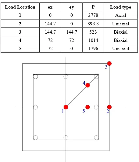
Table 4.2. Balanced Load in different location (Associated with Figure 13)

Load Location ex ey P Load type 1 0 0 2778 Axial

2 144.7 0 893.8 Uniaxial

3 144.7 144.7 523 Biaxial

4 72 72 1014 Biaxial

5 72 0 1796 Uniaxial

Figure 13. Different values of load for different location (Section 300 mm "x300 mm") as per above table

4.5. Some Limitation of Load Contour Method

The graph have some limitation because the graph can be used only for f’c=27.6MPa and fy=415 MPa.

We can overcome this problem quite a bit by using the Section 2.3.

The concrete load carrying capacity is increased as a same percentage as the increase of concrete compressive strength. Similarly the load carrying capacity of steel is increased as a same percentage as the increase of concrete grade.

Because the equation (1) is a linear equation.

Initially we design the column by using f’c=27.6MPa, Fe=415 MPa.

Then we can increase the load or moment as the same percentage if we use high strength concrete and high grade steel.

4.6. Equivalent Method

Biaxial bending means some load make a bending in the X axis and some load in the Y axis.

For the section 300mmX300mm we may divide the load into equal two parts at same distance of e in both directions. That means we can say ex=144.7 mm, ey = 144.7mm, h=300 mm. That means half of nominal load Pn at a distance +144.7mm from both the axis. The maximum nominal load is fall down because this two portion biaxial load creates compression (+) & compression (+) in Zone 1 (Dual compression) & tension & tension in Zone 4 (Dual compression).

We can divide the load into two parts. One 500 KN (Actually calculated value is 523 in Table 4.2, for simplicity we assume the round figure 500 KN) load is placed at a distance +144.7mm from Y axis. And another 500 KN load is placed at the same +144.7mm distance from the X axis. These two loads create compression at right side of the Y axis. And another 500 KN load creates compression in the upper portion of X axis. If we combine the two then we get the combined stress in the column section. The load is fall down because from the concept of Figure 9 we can see that this two loads cause tension in left side of lower side and compression in the upper side of right side. That means the most critical zone in this case is Zone I and Zone III.

From Figure 12 the balanced load is 893.8 KN in case of uniaxial bending.

As the column section is 300 mm X 300 mm so we can assume that the balanced load in biaxial bending is nearly half as that of uniaxial bending.

According to reciprocal method the value of load in Location 3 in Figure 13 is approximately 500 KN. It can be assumed that the maximum balanced load for biaxial bending is half that of uniaxial cases of the same column. But it’s only for the column section with equal b & h.

5. Application of This Study

some floor which affects the neutral axis distance and so on the related values of P & M.

(b) For uniaxial bending column the mid steel perpendicular to the strong axis have no contribution (negligible contribution) in the moment carrying capacity.

6. Conclusions

(a) Balanced failure point is not a single point.

It is defined as a range. In this range for a couple of P & M tension steel or compression steel both yield at the same point.

(b) It’s not possible to get clear idea about neutral axis only from equation (4). For confirmation we need to use the other two equations (1) & (2) as well to define actual balanced load, balanced moment and eccentricity.

(c) In this study the author discussed about neutral axis distance in different condition in different approach and showed that different neutral axis distance affect the load & moment significantly. This should be

checked before selecting proper size of column section/steel ratio/steel placement etc.

(d) The author have an intend to work more on the balanced failure point/zone for biaxial RCC column in their future study.

(e) In the reciprocal load method we need to use some graph to design the biaxial bending column. But the graph is only for f’c=27.6 MPa & fy= 415 MPa. In this case we can design the column for this (For f’c=27.6 MPa & fy=415 MPa). Finally if we use high strength concrete or high grade steel then we increase the design column load as the same percentage what we increase in f’c or fy. In the section 2.3 it is stated clearly.

(f) In the section 3, Case 2 & case 3 is for same column section 300mm X 500mm. The moment carrying capacity is different for different orientation it’s simple. But we see a significant discrepancy in the other value as like as P and C. So to avoid any problem, designer should check all the possibility in different cases in case of high-rise or sensitive structures.

Appendix A Part 1

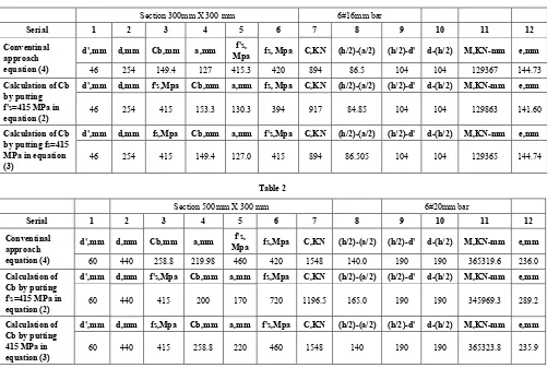
Table 1

Section 300mm X 300 mm 6#16mm bar

Serial 1 2 3 4 5 6 7 8 9 10 11 12

Conventinal approach equation (4)

d',mm d,mm Cb,mm a,mm _{Mpa fs, Mpa C,KN (h/2)-(a/2) (h/2)-d' d-(h/2) M,KN-mm e,mm} f's,

46 254 149.4 127 415.3 420 894 86.5 104 104 129367 144.73

Calculation of Cb by putting f's=415 MPa in equation (2)

d',mm d,mm f's,Mpa Cb,mm a,mm fs, Mpa C,KN (h/2)-(a/2) (h/2)-d' d-(h/2) M,KN-mm e,mm

46 254 415 153.3 130.3 394 917 84.85 104 104 129863 141.60

Calculation of Cb by putting fs=415 MPa in equation (3)

d',mm d,mm fs,Mpa Cb,mm a,mm f's,Mpa C,KN (h/2)-(a/2) (h/2)-d' d-(h/2) M,KN-mm e,mm

46 254 415 149.4 127.0 415 894 86.505 104 104 129365 144.74

Table 2

Section 500mm X 300 mm 6#20mm bar

Serial 1 2 3 4 5 6 7 8 9 10 11 12

Conventinal approach equation (4)

d',mm d,mm Cb,mm a,mm _Mpa f's, fs,Mpa C,KN (h/2)-(a/2) (h/2)-d' d-(h/2) M,KN-mm e,mm

60 440 258.8 219.98 460 420 1548 140.0 190 190 365319.6 236.0

Calculation of Cb by putting f's=415 MPa in equation (2)

d',mm d,mm f's,Mpa Cb,mm a,mm fs,Mpa C,KN (h/2)-(a/2) (h/2)-d' d-(h/2) M,KN-mm e,mm

60 440 415 200 170 720 1196.5 165.0 190 190 345969.3 289.2

Calculation of Cb by putting 415 MPa in equation (3)

d',mm d,mm fs,Mpa Cb,mm a,mm f's,Mpa C,KN (h/2)-(a/2) (h/2)-d' d-(h/2) M,KN-mm e,mm

Table 3

Section 500mm X 300 mm (Orientation) 6#20mm bar

Serial 1 2 3 4 5 6 7 8 9 10 11 12

Conventinal approach

d',mm d,mm Cb,mm a,mm _{Mpa fs, Mpa C,KN (h/2)-(a/2) (h/2)-d' d-(h/2)} f's, _{kKN-mm e,mm} M,

60 240 141.2 120 345 420 1407.6 90.00 90 90 197051.4 140.0

Calculation of Cb by putting f's=415 MPa in equation (1)

d',mm d,mm f's,Mpa Cb,mm a,mm fs,MPa C,KN (h/2)-(a/2) (h/2)-d' d-(h/2) _KN-mm M, e,mm

60 240 415 200 170 120 1994.1 65 90 90 199983.9 100.3

Calculation of Cb by putting fs= 415 MPa in equation (2)

d',mm d,mm fs,Mpa Cb,mm a,mm f's,Mpa C,KN (h/2)-(a/2) (h/2)-d' d-(h/2) _KN-mm M, e,mm

60 240 415 141 120 345 1407.8 89.99 90 90 197058.4 140

Table 4

d',mm d,mm Cb,mm a,mm f's,Mpa fs,Mpa e,mm

60 240 140 119 342.8571 428.5714 60 240 142 120.7 346.4789 414.0845 60 240 148 125.8 356.7568 372.973

60 240 150 127.5 360 360 115.5

Journa

l of C

ivi l E ngi ne eri ng R es ea rc h 2018, 8(3) : 70 -85

A

ppe

ndi

x A

P

ar

t 2

, 8 # 25

m m b ar , f 'c=2 7. 6M Pa, fy =415 M pa Ag 0.2 f'c 27. 6 d' 60 d 440 h 500 b 300 St ee l r at io 0. 026 ex 290 ey 290 ds X 38 0. 0 ds Y 180 Se rial B en din g ab ou t Y ax is B en din g ab ou t X ax is N om in al L oad c alc ulat ion 1 2 3 4 5 6 7 8 9 10 11 12 13 14 15 16 17 18 19 20 21 ex /h G am a (d sX /h ) Fa ct or fr om gr aph 2 Fa ct or fr om gr aph 3 A ve rage fac tor Pn yo fa cto r of Po Po ey /h G am a (d sY /h ) Fa ct or fr om gr aph 1 Fa ct or fr om gr aph 2 A ve rage fac tor Pn xo fa cto r of Po Po 1/ pn xo 1/ pn yo 1/P o

17+ ₁₈-19

(1 /20 ) 0.6 0. 76 0. 34 0. 36 0. 35 144 9 1. 21 5009 0. 97 0. 60 0.3 N/ A 0.3 1242 1. 21 5009 0. 000 8 7E -04 0 0 77 1. 80 8 Ta ble 6 . Lo ad Lo catio n 5 , S ec tion 500 m m X 300 m m

, 8 # 25

m m ba r, f'c =2 7. 6M Pa, fy =415 M pa Ag 0.2 f'c 27. 6 d' 60 d 440 h 500 b 300 St ee l r at io 0. 026 ex 145 ey 145 ds X 38 0. 0 ds Y 180 Se rial B en din g ab ou t Y ax is B en din g ab ou t X ax is N om in al L oad c alc ulat ion 1 2 3 4 5 6 7 8 9 10 11 12 13 14 15 16 17 18 19 20 21 ex /h G am a (d sX /h ) Fa ct or fr om gr aph 2 Fa ct or fr om gr aph 3 A ve rage fac tor Pn yo fa cto r of Po Po ey /h G am a (ds Y /h ) Fa ct or fr om gr aph 1 Fa ct or fr om gr aph 2 A ve rage fac tor Pn xo fa cto r of Po Po 1/ pn xo 1/ pn yo 1/P o

17+ ₁₈-19

2 A. B. M. G ol am Ra bba ny et a l. : Short RCC Col um n P erform anc es in D iffe re nt Con di tions : A xi al , U ni axi al & Bi axi al Be nd ing Ta ble 7 . Lo ad Lo catio n 6 , S ec tion 500 m m X 300 m m

, 8 # 25

m m ba r, f'c =2 7. 6M Pa, fy =415 M pa Ag 0.2 f'c 27. 6 d' 60 d 440 h 500 b 300 St ee l r at io 0. 026 ex 72 ey 72 ds X 38 0. 0 ds Y 180 Se rial B en din g ab ou t Y ax is B en din g ab ou t X ax is N om in al L oad c alc ulat ion 1 2 3 4 5 6 7 8 9 10 11 12 13 14 15 16 17 18 19 20 21 ex /h G am a (d sX /h ) Fa ct or fr om gr aph 2 Fa ct or fr om gr aph 3 A ve rage fac tor Pn yo fa cto r of Po Po ey /h G am a (d sY /h ) Fa ct or fr om gr aph 1 Fa ct or fr om gr aph 2 A ve rage fac tor Pn xo fa cto r of Po Po 1/ pn xo 1/ pn yo 1/P o

17+ ₁₈-19

(1 /20 ) 0.1 0. 76 0. 86 0. 88 0. 87 3602 1. 21 5009 0. 24 0. 60 0. 63 N/ A 0. 63 2608 .2 1. 21 5009 0. 000 4 3E -04 0 0 2167 .22 Ta ble 8 . Loa d L oc at ion 7, S ec tion 500 m m X 300 m m

, 8 # 25

m m ba r, f'c =2 7. 6M Pa, fy =415 M pa Ag 0.2 f'c 27. 6 d' 60 d 440 h 500 b 300 St ee l r at io 0. 026 ex 36 ey 36 ds X 38 0. 0 ds Y 180 Se rial B en din g ab ou t Y ax is B en din g ab ou t X ax is N om in al L oad c alc ulat ion 1 2 3 4 5 6 7 8 9 10 11 12 13 14 15 16 17 18 19 20 21 ex /h G am a (d sX /h ) Fa ct or fr om gr aph 2 Fa ct or fr om gr aph 3 A ve rage fac tor Pn yo fa cto r of Po Po ey /h G ama (d sY /h ) Fa ct or fr om gr aph 1 Fa ct or fr om gr aph 2 A ve rage fac tor Pn xo fa cto r of Po Po 1/ pn xo 1/ pn yo 1/P o

17+ ₁₈-19

Appendix A Part 3

REFERENCES

[1] https://rabbanypalash.blogspot.com/p/guhiuh.html

[2] ACI Committee 318, Building Code Requirements for Structural Concrete (ACI 318-02) and Commentary (ACI 318R-02),” American Concrete Institute, 2002, 10.2.7.3. [3] Arthur H. Nilson, David Darwin, Charles W. Dolan-Design

of Concrete structures-13th _{Edition, “Chapter 08-Short}

Columns,”, McGraw Hill Higher Education, 2006.

[4] CRSI Design Handbook 2008-10th _{Edition, Concrete}

Reinforcing Steel Institute, Illinois, 2008.

[5] A.B.M. Golam Rabbany, Samiul Islam, _Md.

Hasan-Uz-Zaman –“Pile cap performances in different consequences” Architecture Research, 2018 8(2), pp. 51-61, 10.5923/j.arch.20180802.02.

[6] Arthur H. Nilson, David Darwin, Charles W. Dolan-Design

of Concrete structures-13th _{Edition, “Chapter 08-Short}

Columns,”, Page-259, McGraw Hill Higher Education, 2006. [7] https://rabbanypalash.blogspot.com/p/guhiuh.html

[8] STRENGTH AND STIFFNESS OF REINFORCED CONCRETE COLUMNS UNDER BIAXIAL BENDING by V. Mavichak and R. W. Furlong, THE UNIVERSITY OF TEXAS AT AUSTIN November 1976.

[9] Arthur H. Nilson, David Darwin, Charles W. Dolan-Design

of Concrete structures-13th _{Edition, “Chapter 08-Short}

Columns,”, Page-278, McGraw Hill Higher Education, 2006. [10] Arthur H. Nilson, David Darwin, Charles W. Dolan-Design

of Concrete structures-13th _{Edition, “Appendix A-Page}