Statistics for trajectometry
Pierre Billoir
1LPNHE, Paris (IN2P3)
Abstract. A trajectometer is made of layers of charged particle detectors which measure
successive positions along the trajectories; it is generally immersed in a magnetic field, so the curvature of the trajectory provides a measurement of the momentum. A method to perform a progressive fitting of the trajectory (Kalman Filter formalism), incorporating the measurements one after one, with an optimal account for the perturbations (multiple scattering, energy loss), is described with some indications for practical implementations in realistic detector layouts. Useful byproducts of the method and tests of validity are discussed. The procedure appears to be a combinationad libitumof elementary opera-tions on vectors and matrices of fixed dimension (the number of parameters needed to define the trajectory), affording very flexible strategies, including a coupling of the pat-tern recognition of tracks with the fit of the trajectory, and combination with calorimetric or timing measurements. Extension to non-gaussian errors is discussed.
Once the trajectories of an event are independently reconstructed, they may be extrapo-lated back to the region of production of the particles (target, or zone of intersection of the beams in a collider) and associated to one or several vertices (primary interaction, and possible secondary interactions or decays): a fast and flexible method is described to per-form these operations and improve the geometrical reconstruction, hence the kinematical one, by the constraint of a common origin; additional constraints may be added. Here again, the elementary steps consist in linear operations on vector and matrices of fixed dimension, allowing the user to easily proceed by successive trials and to optimize the strategy.
1 Introduction
1.1 What is a "trajectometer"?
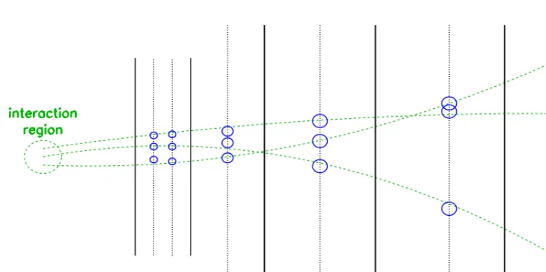
Most of the particle detectors include layers which aim at recognizing and reconstructing as precisely as possible the trajectories of the charged particles produced in the main interaction or in a secondary vertex, usually curved by a magnetic field to provide an information on the momentum. These layers are thin (in terms of radiation lengths) to avoid disturbing the movement. They are generally located close to the interaction point (inner part of the detector for an implementation around a collider, or in first position within a fixed target experiment), before the calorimetric components. However some elements may be set at remote positions to provide a "lever arm" effect for a precise measurement of the curvature: this is the case of external muon detectors, which give both a signature of muons and a relatively precise measurement of their position. A schematic layout of a trajectometer is shown in Fig.1, in the case on planar layers; for a detector installed around the intersection region of a collider, a better description is obtained by replacing the planes by cylinders.
C
Owned by the authors, published by EDP Sciences, 2013
Figure 1. Schematic layout of a trajectometer. The green dashed lines are the trajectories of charged particles coming from the interaction region. The solid black lines are layers of material, the dotted black lines are measurement layers. The measurements are the blue circles (with a radius proportional to the uncertainty).
1.2 What is known and what is searched for ?
The following properties of the detector are supposed to be known (or determined at a previous stage from calibration data):
• the equation of propagation, which determines the shape of the trajectories. In practice, it is defined by the magnetic field map within the trajectometer.
• thenatureand theprecisionof the measurements (drift time, amplitude on signals in strips or pads, etc). In simple cases they just give one coordinate or a fixed combination of coordinates. They may also depend on the direction of incidence on the detection layer. In practice, what is needed is to express the measured quantity as a function of the local parameters of the trajectory (position and direction). The distribution of errors is generally gaussian, but possible exceptions should be evaluated and accounted for.
• the nature and the amplitude of the "noise" processes (random perturbations of the trajectory): the multiple Coulomb scattering, which modifies the direction, and the fluctuations of the energy loss, which affect the curvature. These perturbations depend on the amount and the nature of the material crossed by the particles, but also on their momentum. As a consequence, a good approximation of the momenta (or their inverse) has to be given by an external information (e.g. a calorimetric measurement), or by a first reconstruction where these perturbations are neglected.
• the properties of each particle (momentum, direction) at its origin. In practice, we want to obtain a backward extrapolation to the interaction region (the interior of the beam pipe for a collider), or to a secondary vertex of production. A magnetically curved trajectory may be described, when crossing
a given reference surface (for example, for a given value of coordinatex), by 5 parameters: two for
the position of the intersection with the reference surface (e.g.y,zfor the example above) and 3 for the momentum vector (or the momentum and two angles). We suppose here that the mass is known or irrelevant; if not, several reconstructions may be needed, for different mass hypotheses.
• in some cases: a forward extrapolation towards external parts of the detector: e.g. the entry point
into a calorimeter of into external muon chambers.
• the position and the composition of the primary vertex and secondary vertices within the detector,
if any. This includes making one or several association of particles, and to use the constraint of a common origin to improve the reconstruction at the origin. Here again a procedure using iterative trials may be needed.
1.3 The problem of the noise
If the noise processes have negligible effects, we can choose a set of "initial" parameters p0(position,
direction, momentum) which gives a deterministic prediction of the expected measurements in layer k: ¯mk=Fk(p0). Because the measurement errors are independent we can write aχ2to be minimized:
χ2=
k
mk−Fk(p0)
σk 2
wheremkis the actual measurement, with an errorσk. If needed (significantly non-gaussian errors),
this may be replaced by a log-likelihood which is also a sum of independent terms. In most detectors
the errors are small, so starting from a first approximation of the trajectory,Fkmay be replaced by
a linear function of the parameters and minimizing theχ2 consists in solving a linear system ofn
p
equations, wherenp is the number of parameters. An iteration may be needed, but in general, the
computation is fast.
The situation is more delicate if the errors induced by the noise are comparable to the measurement errors, or larger : a perturbation on the particle affects all measurements coming afterwards, so the
measurements are no longerindependent. Theχ2should now be written as:
χ2=
j,k
Wjk(mj−Fj(p0))(mk−Fk(p0))
whereWis the inverse of the total covariance matrix, including the measurement errors and the noise
induced errors, with non vanishing covariance terms: the measurementsmj andmk are correlated
through the perturbations occurring before both of them. This requires heavier computations;
moreover, to make an optimal forward extrapolation we need to evaluate another covariance matrix,
wheremjandmkare correlated through the perturbations occurringafterthem.
In the following sections we apply to trajectometry an alternative method better suited to estimate
the state of a dynamic system affected by random perturbations: the Kalman Filter (KF). The
pre-sentation differs slightly from the traditional one, but it is mathematically equivalent. Here we use
systematically aweight matrixandweighted meanformalism, which has the advantage of being more
more or less details the operations within some frameworks (for example for some choices of parame-ters to define the trajectory), but we cannot give an exhaustive review of all possible implementations: the tools need to be adapted to a given context, after a clear understanding of the detector and the possible and useful approximations. In any case, the choices should be dictated by the gain in terms of the precision on physical quantities of interest for a further analysis.
2 The principle of the Kalman Filter (progressive fitting): a simple
unidimensional example
2.1 The simplest model of measurement of a "noisy" process
We consider here a point with a random motion on a line. Its position x(t) is measured without
bias at times 1,2,3,· · ·, with independent measurement errors of varianceσ2. The displacements
between two measurements are 0 in average and independent, with the same varianceτ2(for example,
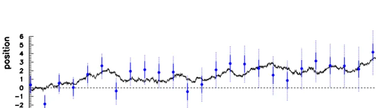
this is a brownian motion, as illustrated in Fig.2). The measurement errors are independent of the displacements.
Our problem is: if we haven successive measurementsXk of the true positions xk, what is the
combination of theXkgiving the best estimator of the initial positionx1, or the final onexn? and why
not, the best estimator of any intermediate positionxk? The solution is simple ifτ2is negligible (at
any time: the average of the measurements), or ifτ2 is very large compared toσ2(the best forx
kis
justXk, because the other measurements are too much disturbed). It is less clear ifτ2is comparable
toσ2, or, more precisely, ifnτ2(the total variance of the displacements) is comparable toσ2: in that case, the cumulated displacements and the measurement errors cannot be disentangled.
Figure 2. Measurements (blue points) of the position of a point moving randomly on a line. Here a brownian motion is simulated (solid line), and the variance of the displacement between two measurements isτ2=0.25. The solid bars represents measurement errors withσ2 =1; the dotted ones include the contribution of the displacements from the beginning, i.e. for
pointkit is√kτ2+σ2.
A first solution we may think about is the following: the difference betweenXkandx1is the sum
of (k−1) independent displacements and one measurement error, so its variance isVk=(k−1)τ2+σ2.
We could make theweighted averageof theXk, with weights equal to 1/Vk. This would be actually
the best linear estimator, if theXk−x1wereindependentrandom variables; butthis it not truein our
problem, because they include all displacements from the beginning: XkandXlboth depend of the
To build the best estimator in a standard way, we have to account for the (n ×n) covariance
matrixCof theXk. A linear combination
akXkis an unbiased estimator ofx1 if
ak =1 and its
variance is minimal ifajakCjkis minimal within the above constraint. That is, we have to solve a
linear system ofnequations; the solution may be written as a weighted mean of theXk, with weights
wk=j(C−1)jkXj. The complexity of the problem grows more than linearly withn. Moreover, if we
want to evaluate the final position, or an intermediate one, we have to build another covariance matrix and then solve a different linear system.
Fortunately, there is another way to obtain the same results, with a number of operations
propor-tionaltonthrough the Kalman Filter methodology [ 1, 4] (progressive fitting[2, 3]).
2.2 Tools of the progressive fitting
The fundamental idea is to incorporate the measurementsone after onein the algorithm, in such a
way thatindependentrandom variables are combined at any stage. The procedure is illustrated on
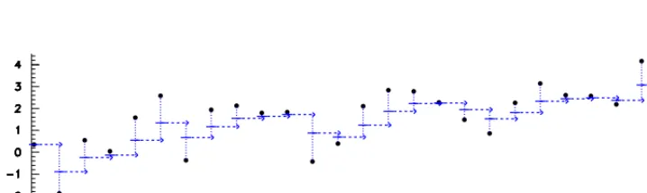
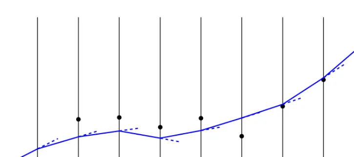
Fig.3, which may help to understand the simple operations behind the mathematical formulae.
Figure 3.Principle of the forward filter, applied to the same dataset as in Fig.2 (the black points are the measurementsXkof
the successive positionsxk). The blue solid line at timekrepresents ˜X1→k,k, best estimator ofxkusing the firstkmeasurements
(see text below), which is combined with the next measurementXk+1to give ˜X1→k+1,k+1, best estimator ofxk+1, and so on.
Let us consider the following elementary steps:
• X1 = x1+ε1 = x2−η1+ε1, whereε1 is the measurement error on point 1 (varianceσ2) andη1
the displacement from time 1 to time 2 (varianceτ2). Becauseε
1andη1 are independent, we see
thatX1−x2has a varianceσ2+τ2, that is,X1is equivalent to a measurement ofx2with variance
σ2+τ2.
• By definition,X2 = x2+ε2is another measurement ofx2, with varianceσ2. The crucial point is
thatε2isindependentof bothε1andη1, soX1andX2are twoindependentmeasurements ofx2. • The "best" linear combination of two independent measurements (that is, with the lowest variance)
is their weighted mean with weights equal to the inverse of their variance. Here, this means that the "best" combination ofX1andX2to estimatex2is:
˜ X1→2,2=
X
1
σ2+τ2 +
X2
σ2
/
1 σ2+τ2 +
1 σ2
of variance ˜σ21→2,2=1/
1 σ2+τ2 +
1 σ2
(where the notation ˜Xl→m,kmeans: best estimator ofxkusing measurementsltom).
In the case of gaussian errors, the steps described above may be interpreted as operations on a likelihood functionL: including only the measurementX1ofx1,Lis a gaussian function; accounting
for the random displacement consists in aconvolutionwith another gaussian function; combining two
independent measurements is a multiplicationof the corresponding gaussian functions. Of course,
maximizingLgives the same results as above. We will see later that this formulation can be extended
to more complex cases.
The remarkable feature of this algorithm is that it can be iterated to include a further measurement (for convenience we replace ˜σ1→2,2by ˜σ):
• X˜1→2,2 found above is a measurement of x2 with variance ˜σ2, so it is a measurement ofx 3 with
variance ˜σ2+τ2
• X3is another measurement ofx3, with varianceσ2, andX3−x3 =ε3is independent of all random
variables used to build ˜X1→2,2.
• so we obtain the best linear combination ofX1,X2,X3to estimatex3:
˜ X1→3,3=
˜
X1→2,2
˜ σ2+τ2 +
X3
σ2
1 ˜ σ2+τ2 +
1 σ2
of variance 1 1
˜ σ2+τ2 +
1 σ2
Let us note that this may be written in a simpler way using the formalism of theweight(inverse of
the variance) to express the combination as aweighted mean: 1
˜ X1→3,3=
˜
w1→2,2X˜1→2,2+w3X3
˜
w1→2,2+w3
The variance is 1/( ˜w1→2,2+w3), in other terms: the weight of the combined estimator is just the
sum of the weights of the two independent estimators.
We can in the same way incorporate the fourth measurement, and so on, and build ˜X1→k,k
suces-sively for all values ofk. This is the "forward filter", which gives eventually the best estimator of the final position. It is clear that we can obtain the best estimator of the initial position through a similar formalism, starting from the last measurement and incorporating the other ones in reverse order. This is the "backward filter", giving, with our notations, ˜Xk→n,kfor anyk. This is convenient if we have in
mind a particle detector, where we are mainly interested to the initial parameters. We can also build aχ2
minassociated to each step of the procedure, in the usual way: • combiningX1andX2to estimatex2, we have
χ2(X)=(X−X
1)2/(σ2+τ2)+(X−X2)2/σ2
thenχ2min =(X1−X2)2/(2σ2+τ2)
• at any further timek+1 we combine ˜X1→k,k+1 ( ˜σ12→2,2,χ2min,k) withXk+1. This gives a new value χ2
min,k+1=χ2min,k+(Xk+1−X˜1→k,k)2/( ˜σ12→2,2+σ2)
As usual, in the gaussian case, χ2
min = −2 ln(Lmax), where Lis the likelihood, omitting a constant
normalization factor, and it follows the law ofχ2withN−1 degrees of freedom,Nbeing the number
of measurements included.
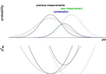
The principle of one step of the filter is illustrated in Fig. 4.
1In the usual presentation of the KF, this step would be expressed as: find the best combination ˜X1
→2,2+λ(X3−X1˜ →2,2),
Figure 4. The estimator including all measurements up to a given point is represented in black (top: density of probability; bottom: minimum ofχ2), the dotted line accounts for the next random displacement. The green line represents the next measurement, and the blue one is the combination of these two independent estimators, which is the input for the next step.
2.3 Useful byproducts
We can build further tools with very few more efforts: it is easy to obtain the best estimator of any
intermediate position using all measurements, that is, to build the "smoother" in the KF terminology
(optimalinterpolation), by an adequate combination of the forward and backward filters. The forward
filter gives ˜X1→k,kas an estimator of xkwith a variance that we callσ2f, and the backward one gives
˜
Xk+1→n,kwith a varianceσb2(including a termτ2to go from ˜Xk+1→n,k+1to ˜Xk+1→n,k) ; these estimators
include independent measurement errors; the key point is that they also includeindependent
displace-ment errors(theηjwith 1≤ j≤kfor the forward one,k< j≤nfor the backward one). So they can
be simply combined as a weighted mean, definingwf =1/σ2fandwb=1/σb2:
˜ X1→n,k=
wfX˜1→k,k+wbX˜k+1→n,k wf +wb
The same result is obtained by combining ˜X1→k−1,pand ˜Xk→n,k with their proper variances (we just
need to include Xk once and only once). We can also write anexclusiveinterpolation (without the
possible outliers, as discussed below.
Up to now we have assumed a perfect situation: both the displacements and the measurement errors have the expected distribution. In practice, in particle detectors, there may be deviations due to rare phenomena affecting the trajectory (e.g. a hard scattering), bad measurements or bad assignments of points to a given trajectory (especially if many particles cross the same detector element). It is useful to build tools to detect abnormal deviations ("outliers") and to define a strategy to get rid of them, as far as possible. Within our very simple model we can define two kinds of tests which can be extended to realistic situations:
• for a given timek, the difference ˜X1→k,k−X˜k+1→n,k between the forward and the backward filters
has a predicted standard deviation σ2
f+σ
2
b+τ2. If σ
2
f +σ
2
b is smaller or comparable toτ
2,
displacements which are large compared toτmay be detected; if not, the test can only discriminate
very large deviations. If the distribution of the measurement and displacement errors are gaussian, a probability ofχ2may be used as a discriminator.
• for timek, the measurementXkand the exclusive interpolation (of varianceσ2e) are independent,
therefore the variance of their difference isσ2
e+σ2. Here again, ifσ2eis not too large compared to
σ2, outliers (abnormal measurements) may be detected. In the gaussian case, the probability ofχ2
gives a good discriminator.
Finally, let us remark that a large sample of clean measurements may be used to perform a
cali-brationof the errors: ifσandτare not knowna priori, the distribution of the residuals mentioned above provide estimators for them, and possibly some hints on the distribution of errors.
2.4 Comments
The Kalman Filter was originally suited to dynamical problems like following the trajectory of en-gines from successive observations. In that case, the forward filter is the most natural tool: it can give in real time an updated estimation of the present state (position, direction, velocity). In applications to particle trajectometry, computations are not done in real time: even if some algorithms are imple-mented online, their input is a set of measurements coming after the particle has escaped the detector. Moreover the main purpose of the reconstruction of trajectories is to provide the best estimations at starting point (ideally, the vertex where this particle is originating from), so the backward filter is the basic tool. However, extrapolations to external detectors and interpolations may be needed, and discrimination of outliers is quite useful.
The number of operations to build the complete set of filters (forward, backward and smoother)
is proportional ton if no outliers are removed. However, if a pointkis to be removed after being
compared to the interpolation, the forward filter has to be reevaluated at all points afterk, and the
backward filter at all points beforek; the smoother has to be redone everywhere.
3 More complex examples
In these examples, we want to go progressively to the description of a real detector. In particular, we do not consider measurements labeled by times, but measurements of one or several coordinates as functions of one coordinate describing the successive layers of the detector. To simplify some
expressions we will use the following notations for matricesA,Band vectors q:
3.1 Straight line planar trajectory (2 parametres, linear model)
In this example (illustrated in Fig.5) the trajectory may be described asy=ax+b, and the coordinatey is measured asYkatxk(k=1,x,· · ·n), with a varianceσ2k. The noise consists in a random scattering
(variation of the slopea) with a varianceρ2
k at each measurement layerxk2. All measurement and
scattering errors are independent .
Figure 5. A planar trajectory made of straight line segments between measurement planes, where the slope is randomly modified (simple model for the multiple scattering on particles). The black points represent measurements.
The parameters to be fitted areaandb; we call p the vector (b,a), or, more generally the vector oflocalparameters (y,dy/dx) at any point of the trajectory. LetCbe the (2×2) covariance matrix of an estimator, andW its inverse (theweight matrix). If all errors are gaussian, the log-likelihood is a quadratic function of p:
−2 ln(L)=−2 ln(L)max+W p−˜p
where ˜p is the best estimator. In the general case, we will build the "best" linear estimator (using all
measurementsYkup to a given position) through linear combinations using the matricesCand/orW
at different stages of a progressive fitting procedure.
Before that, we will try to analyze this problem of estimating (a,b) with the standard method,
by computing the variance/covariance of the measurements. We callεk the error onYk andζk the
variation of slope atxk. Then:
Yk=axk+b+εk+
j<k
(xk−xj)ζj
var(Yk)=σ2k+
j<k
(xk−xj)2ρ2j
2 We supposeρ
kto be knowna priori. For a physics interpretation in terms of multiple scattering, this means that the
cov(Yk,Yl)=
j<inf(k,l)
(xk−xj)(xl−xj)ρ2j
The best linear estimator is obtained by minimizing the globalχ2:
χ2=
j,k
Wjk(Yj−axj−b)(Yk−axk−b)
that is, we have to invert the (n×n) non-diagonal covariance matrix of the measurements.
Let us now describe one step of a progressive procedure; for convenience we will uselocal
pa-rameters (the value ofyatxkand the slopea). For the moment we suppose that we have built the best
estimator ˜p1→k,k(matrices ˜C1→k,k, ˜W1→k,k) usingY1,Y2· · ·Yk, associated the a minimum value ˜χ21→k,k,
and we want to build ˜p1→k+1,k+1. We have to perform 3 operations:
• account for the scattering atxk, by evaluatingCfor ˜p1→k,kas an estimator of the parametersafter
the scattering. In our model, we just need to account for an additional error ona, so we compute:
˜
C1→k,k=C˜1→k,k+
0 0
0 τ2
and W˜1→k,k=( ˜C1→k,k)−1
The value of ˜χ2is not modified.
• propagatethe estimator, going to the local parameters atxk+1: we haveyk+1=yk+a(xk+1−xk), and
the slopeais not modified. We write this simple transformation in a matrix formalism:
˜p1→k,k+1=Dk→k+1 ˜p1→k,k with Dk→k+1=
1 xk+1−xk
0 1
˜
C1→k,k+1=C˜1→k,k
DTk→k+1
W1→k,k+1=W˜1→k,k[Dk+1→k] using (Dk→k+1)−1 =Dk+1→k
• combine˜p1→k,k+1with theindependentinformation given byYk+1. The combinedχ2is:
χ2(p
k+1)=χ˜21→k,k+W˜1→k,k+1 pk+1−˜p1→k,k+1+
(Yk+1−y˜1→k,k+1)2
σ2
k
We introduce now the 2-vector oflocal measurementPk+1=(A,Yk+1) and itsweight matrix
Wkm+1 =
1/σ2k 0
0 0
ActuallyAis not measured, but the expression ofχ2does not depend on it; we can set it to 0 by
convention. With these definitions we have to minimize:
χ2(p
k+1)=χ˜21→k,k+W˜1→k,k+1 pk+1−˜p1→k,k+1+Wkm+1
pk+1−P˜k+1
The solution may be written as:
˜p1→k+1,k+1=( ˜W1→k,k+1+W m k+1)−
1( ˜W
1→k,k+1˜p1→k,k+1+Wkm+1P˜k+1)
which is an extension of the weighted mean found in the simplest model (here the weights are
matrices). We still have the property ofadditivity of weights: the weight matrix of the combination
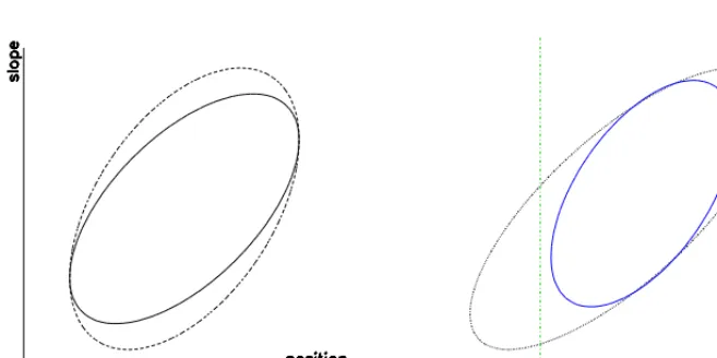
Figure 6. The operations of one stepk→k+1 of the filter (as in Fig.4) applied to a 2-parameter model (position and slope of a trajectory). The ellipses are the contours associated to one standard deviation around the central value. Left: solid: the "initial" estimator ˜p1→k,k; dashed: including the scattering. Right: black,dotted: propagated to pointk+1; green, dash-dotted:
measurement Pk+1at pointk+1 (position only→vertical strip); blue: combination.
The formalism above may be completely expressed with elementary operations on "atoms" of information (one "atom"=vector of local parameters+weight matrix+minimalχ2), but we have
evaded some technical problems for a practical coding of the algorithm, especially: how to begin this recursive procedure. With the first measurement we have not enough information to define both parameters: we have seen that we can manage this situation by taking a singular weight matrix
diag(1/σ2,0) and a measurement vector with an arbitrary value for the first element (0 for
exam-ple): theχ2 valley may be seen a strip in the (a,b) plane, along theadirection. This "atom" may
be propagated to the next position with the formalism above: the valley is still infinite, by now in
an oblique direction w.r.t. the local parameters; when combined to a strip in theadirection (local
measurement) it results in a finite region, and both ˜Cand ˜Ware regular.
The handling of the scattering remains to be clarified, because the operation ˜C = C˜ +Cscat
cannot be done if ˜C is not yet defined (first point). However we can rewrite this operation as
˜
W=( ˜W−1+Cscat)−1=(1+WC˜ scat)−1W˜, which can be performed with one measurement only.
3.2 Further comments
The forward filter and the interpolators may be defined in the same way as in the simplest model. The
tools to detect measurement outliers or abnormal scatterings may be built usingχ2 differences, with
the same principles.
In the previous model the scattering occurred at the positionsxkwhere measurements were done.
The formalism may be extended to any configuration: we just need to define the set of positions xk
where something happens (measurement or scattering) and to make the corresponding operations on (p,W, χ2) by increasingx(forward filter) or decreasing x(backward filter), with propagation
outside the range of measurements. An important application is the material between the vertex of ori-gin and the first measurement (e.g. the beam pipe), to be accounted for in the analysis of the primary interaction.
A thick scattering region may be described, either as a set of elementary layers handled as above, or globally by computing the (2×2) matrixCscat: at first order, the scattering through a thick material
is fully described by terms to be added to the covariance matrix ofyandaat a given reference position x0, including a non-diagonal one to account for their correlation.
3.3 Curved planar trajectory (3 parameters)
Here we want to introduce a good approximation of a detector making measurements in a plane xy
perpendicular to a magnetic field, for trajectories with a moderate angle w.r.t. thexaxis, and a large radius of curvatureRcompared to the size of the detector. In that case we can describe the trajectory with a linear function of 3 parametersa,b,c:
y=ax+b+x2/2R=ax+b+cx2/2
We assume as above thatyis measured atxk(k=1,2,· · ·n) with a varianceσ2k. The 3-vector of local
parameters is p=(y,dy/dx,d2y/dx2). In this model we can account for scatterings (random variations
of dy/dx) and also for both deterministic and random variations of energy, which are expressed as
variations of the curvature d2y/dx2. The formalism of the filters is exactly the same as in the previous
model (plus a specific operation to modify the curvature parameter in case of energy loss), with a few technical differences:
• The matrixW is regular only when at least 3 points are included in the fit. In practice, it is of rank 1 with one point (theχ2valley is a slice in 3D space), 2 with 2 points (theχ2valley is a tube). But
the same formalism as above may be used: a measurement is represented by a vector (Yk,0,0) with
weight matrixdiag(1/σ2,0,0) and in the initial vector of parameters undefined values are set to 0.
• In this model the momentum may be estimated from the fit itself so the variance of the scattering
angles may be computed without external information; more precisely: the relevant curvature
pa-rametercis proportional to the inverse of the momentum, with a geometrical sign depending on the
physical sign of the charge, which is also to be determined. However, the curvature is not supposed to be known at the beginning of the filter. As a consequence, an iteration is needed: for example, the trajectory is fitted first ignoring the scattering, and the curvature found is injected in a second pass; if the curvature is significantly modified, a third pass may be needed. If the measurement range is too short to provide a significant estimation of the curvature, an external information is needed to use the noise formalism in the filters.
3.4 Realistic trajectory in space: using a linear approximation
In real detectors, no linear model (as the parabolic one) may represent the trajectories with the accu-racy requested by the precision of the measurements. However, if the magnetic field is regular, one can choose initial parameters such that the position and the direction of the trajectory in any
mea-surement layer depends smoothly on them3. In these conditions areference trajectorydetermined by
3this may be wrong for low energy particles at the end of their range, but in that case the contribution of the noise is so large
initial parameters p0may be defined as a first approximation, such that the functionsFkintroduced in
Sect.1.3 may be replace by alinear expansion:
Fk(p0+δp)=Fk(p0)+(∇F)0.δp
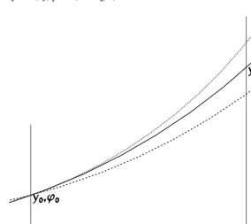
Let us take an example to illustrate a practical application of this method (and possible limitations): a circular trajectory in a (xy) plane (see Fig.7).
Figure 7. A planar circular trajectory measured at fixedx. Solid: the reference trajectory; dashed: with a variation of the initial directionϕ0; dotted: with a variation of the curvaturec(changing the initial positiony0gives a simple translation). The
parameters atx1(y1, ϕ1) depend linearly on small variations of the initial parameters atx0.
The initial parameters (atx=0) arey0, ϕ0,c=1/R, whereϕis the local direction (tanϕ=dy/dx)
andRthe radiusRwith ageometrical sign: by convention we take+for an anticlockwise trajectory;
in this modelcis constant. With our convention we can write:
x=x0+R(sinϕ−sinϕ0) y=y0+R(cosϕ−cosϕ0)
First we want to evaluate the parametersy1, ϕ1,cat a fixed abscissa x1. The first equation gives
two solutions forϕ1(or no one !), and we have to choose one of them. In general it is the nearest one
toϕ0(but an actual measurement can correspond to the second solution if it is within the detector...).
Once the “right” solution (y1, ϕ1) is found, we want compute the derivatives of ofy1, ϕ1w.r.t.y0, ϕ0,c.
Differentiating the first equation we obtain the derivatives ofϕ1(withΔx=x1−x0):
dϕ1=
cosϕ0
cosϕ1
dϕ0−R2Δx
cosϕ1
dR → ∂ϕ∂ϕ1
0
=cosϕ0
cosϕ1
; ∂ϕ∂1 c =
Let us now differentiate the second one:
dy1=dy0−(cosϕ1−cosϕ0)dR+R(sinϕ1dϕ1−sinϕ0dϕ0)
Injecting the expression ofdϕ1 found above in this equation, we can extract after some algebra the
derivatives ofy1:
∂y1
∂y0 =
1 ∂ϕ∂y1
0 =
sin(ϕ1−ϕ0)
ccosϕ1
∂y1
∂c =
1−cos(ϕ1−ϕ0)
c2cosϕ 1
It is interesting to note that whenRis large,cis a more convenient parameter thanRorR: in that case ϕ1−ϕ0is small and proportional toc, so all derivatives go to a finite limit whenR→ ∞; moreover, the valuec=0 (straight line, infiniteR) is not a singularity, and the geometrical sign may freely change during a progressive fit.
These expressions give us the expression of the 3×3 propagation matrixDsimilar to the 2×2
matrix defined in Sect.3.1. We give in parentheses the approximation for weakly curved trajectories (smallΔϕ), introducing the length of the arc between the two points= Δϕ/c
D= ⎛ ⎜⎜⎜⎜⎜ ⎜⎜⎜⎜⎝ 1
sin(Δϕ)
ccosϕ1 (
cosϕ1)
1−cos(Δϕ)
c2cosϕ1 (
2
2 cosϕ1)
0 cosϕ0
cosϕ1 ( 1)
Δx
cosϕ1 ( )
0 0 1
⎞ ⎟⎟⎟⎟⎟ ⎟⎟⎟⎟⎠
This formalism should be used with care when the trajectory is close to a real singularity (quasi
tangent to the measurement layer, that is cosϕ1 0): then the linear approximation is no longer valid,
and moreover the actual meaning of the measurement may not be the coordinatey, and depend on
the internal structure of the detection layer. In such a situation, it may help to redefine the parameters
(e.g. take xat fixedy) and to express specifically the response of the detector under a skimming
incidence; if this is not possible, the best solution is to ignore the measurement.
Once a convenient parametrization and a reference trajectory are found, the linear formalism using
weight matrices may be applied to the vectorδp. TheCandWmatrices are the same for p andδp. If
the deviations from the reference are too large, it may be iteratively redefined until a satisfactory one is found. It is also possible to use different references for different parts of the trajectory; to go from one part to the next one, the parameters and their weight matrix need to be transformed through an operation similar to the propagation described in Sect. 3.1 (see below).
3.5 Convenient parameters in usual detector configurations
We consider here two main categories of detectors: fixed target experiment or collider. In the first case
the detection layers are mainly planes perpendicular to the beam axis (zcoordinate) in the forward
region, and possibly planes parallel to the beam around the target; in the second one there is a “barrel”
part (cylinders of axis alongz) and endcaps (planes perpendicular toz). Other configurations are
possible, for example with “oblique” layers; this will be discussed later. If there is a magnetic field,
we will useS/pto describe the curvature (pis the momentum,S the physical sign). In some cases
(e.g. roughly uniform field alongz) it is more convenient to useS/pt(ptis the transverse momentum).
3.5.1 Cartesian parameters
3.5.2 Cylindrical parameters
If the detection layers are cylinders around the beam axis, cylindrical coordinates (r,Φ,z) are natural parameters for the position: more precisely, the position at fixedr(in a detector layer) is defined by Φ,z(optionallyrΦ,zfor homogeneity). The direction may be given byθ, ϕ4. If the field is uniform
and parallel tozaxis, the trajectory is a helix of radiusR. As in Sect. 3.4, we useRwith a geometrical sign (+if the trajectory is anticlockwise inxyprojection). Using a pointx0, y0,z0 on the trajectory
andϕas a running parameter, the trajectory is defined by:
x = x0+R(sinϕ−sinϕ0)=r0cosΦ0+R(sinϕ−sinϕ0)
y = y0− R(cosϕ−cosϕ0)=r0sinΦ0+R(cosϕ−cosϕ0)
z = z0+Rcotθ(ϕ−ϕ0)
3.5.3 The “perigee” parameters
It may be useful to summarize the information about the trajectory in one set of intrinsic parameters instead of using an arbitrary reference surface. In the case of quasi-uniform magnetic field along the
beam axis (by convention thezaxis), we can use the “perigee”, point of closest approach to thez
axis: if the particle originates from the main vertex, this point will be close to this vertex, so it will give a good approximation of the particle momentum. Another advantage is that a propagation of the trajectory and its error matrix to this point includes most of the material actually crossed by the particle (all material if the perigee is within a vacuum region, e.g. the beam pipe), so if this material is taken into account properly, the perigee parameters may be used in a further step of vertex fitting in a purely geometrical way, without accounting for noise: this will be exploited in Sect. 6.
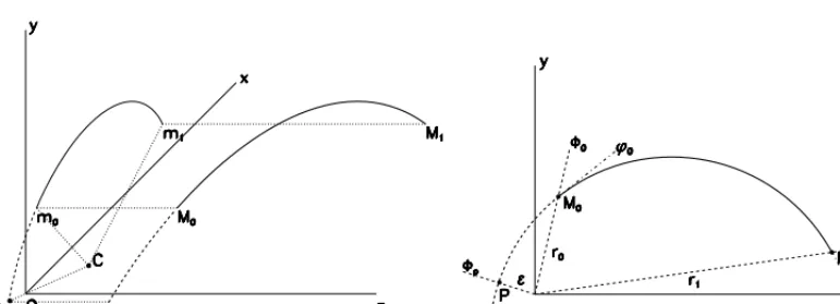
The trajectory is defined by 5 parameters (see Fig. 8 ): the cylindrical coordinates of the perigee (ε,Φp,zp), the signed curvature c = 1/Randθ. To avoid discontinuities around the origin when
extrapolating a trajectory towards the interaction region, it is convenient to give a geometrical sign toε: by convention it is positive if the originOis on the right hand side of the trajectory, andΦp
is defined asϕp+π/2. With this convention, we have alwaysxp =εcosΦp,yp =εsinΦp, and the
trajectory may be parametrized as:
x = εcosΦp+R(sinϕ−sinϕp)=εcosΦp+R(sinϕ+cosΦp) y = εsinΦp− R(cosϕ−cosϕp)=εsinΦp− R(cosϕ−sinΦp)
z = zp+Rcotθ(ϕ−ϕp)=zp+Rcotθ(ϕ−Φp+π/2)
In the vertex fitting procedure, we need in principle short range extrapolations from the perigee, so
we can use the second order approximation in = R(sinϕ−sinϕp) (distance from perigee in xy
projection):
x = εcosΦp+sinΦp+c2cosΦp y = εsinΦp−cosΦp+c2sinΦp
z = zp+cotθ
The perigee parameters will also be used as a technical tool to compute the derivative matrices needed to propagate the error matrix in cylindrical coordinates (see Appendix).
Figure 8.Left: the trajectory in 3D-space (helix of axis alongz). Solid: the measured portionM0M1, dashed: the extrapolation
to the perigeeP. Right: The projection onto thexy(circle). The position of a point along the trajectory is defined byr,Φ; the direction of the tangent is defined byϕ. In this example, the signed radiusRis negative (ϕdecreases with increasingr), and the perigee distanceεis positive.
3.5.4 Propagation of error matrices
In the helix model for trajectories, the analytical computation of the matrix of derivativesDwas done in Sect.3.4 for cartesian parameters. Using similar techniques, on can obtain analytical expression for cylindrical parameters, as function of the parameters at the initial and the final point. The computation is developped in Appendix.
If the magnetic field is not perfectly uniform, the trajectory has to be propagated with a preci-sion better than the measurements, so a numerical computation (or a perturbative expanpreci-sion) may be needed. However, the derivatives may be taken from the analytical expressions, because they give a sufficient approximation for the propagation of errors.
3.5.5 Local change of parametrization
To follow the disposition of the detector layers, it may be convenient to modify the parametrization at a certain point of the trajectory. For example, with the helix model in cartesian coordinates, we use parameters (x, y, θ, ϕ,c) at fixedzin the forward region, and (x,z, θ, ϕ,c) at fixedyin the lateral
region. Here using the same notationxfor a parameter with a different meaning may be a source of
confusion: the transformation of the error matrix should account for a non trivial transformation on the position parameters: an elementary variationδyofyin a planez=z0, at given values ofx, θ, ϕ,c,
is a translation which results in a displacement of the intersection of the trajectory with a plane at fixedy; using the notationa|bfor “aat fixedb”, and noting u the unit vector along the trajectory, the
variations of the coordinatesx|y,z|yare:
δx|y=−ux
uyδy|z=−cotϕ δy|z ; δz|y=−
uz
uyδy|z=−
cotθ sinϕδy|z
For the same reason, if the curvature is not negligible, a variation ofy|zwill affect the direction
model:
δϕ=cδ=− c sinϕδy
The jacobian matrix of the transformation from (x, y, θ, ϕ,c)|zto (x,z, θ, ϕ,c)|yis then:
Dloc=
⎛ ⎜⎜⎜⎜⎜ ⎜⎜⎜⎜⎜ ⎜⎜⎜⎜⎜ ⎜⎜⎜⎜⎝
1 −cotϕ 0 0 0
0 −cotsinϕθ 0 0 0
0 0 1 0 0
0 − c
sinφ 0 1 0
0 0 0 0 1
⎞ ⎟⎟⎟⎟⎟ ⎟⎟⎟⎟⎟ ⎟⎟⎟⎟⎟ ⎟⎟⎟⎟⎠
The covariance and the weight matrix are modified asCnew = ColdDT
loc
= DlocColdDTlocand
Wnew=WoldD−1 loc
=(D−1
loc)
TWoldD−1 loc.
For any other change of local parameters, a similar study has to be done to define the jacobian matrix.
3.6 Indirect measurements of parameters ("oblique" projection)
Up to now we have represented a layer of by a simple surface (e.g. a plane of wires). The quantity ac-tually measured by a detector is supposed to depend on the position of the intersection of the trajectory with this surface, but it may also depend on the direction of incidence. Let us take two examples:
Figure 9.Examples of “oblique” measurements. The trajectory (blue line) has a slopea=dx/dz. In both cases,xmrepresents
the coordinate effectively measured in the planez=z0through a raw measurement in the detector. Left: the raw measurement
• In a planez=z0, we mesure the distance of closest approach of the trajectory to a wire atx=x0(see
Fig.9, left). Using the parametersxanda =dx/dz, and assuming that the curvature is negligible
at this scale, this means that we measured =|x−x0|/√1+a2, with a precisionσ. Within a good
approximation, we can take the reference valuearef of the slope, and consider that we measure
x=x0±d
1+a2
refwith a precisionσx=σ
1+a2
ref(at this level there may be an ambiguity if
the extrapolation provided by the filter is not precise enough).
• The detector surface is not exactly perpendicular toz axis (see Fig. 9, right). For example, we
measure a coordinateξin a plane inclined byαon the xyplane, intersecting the planez = z0 at
x=x0(ξ=0 at the intersection). We obtainx−x0=(cosα+arefsinα)ξ. Here again we apply to
the measurement a factor depending on the local direction.
The real situation may be more complex. For example, in a drift chamber, the relation between the measured time and the local parameters depends on the position (close to the wire or far away). Or we may have to consider in a barrel detector (with cylindrical parameters) detector elements which are planar. In any case, the prescription is to write the local parameter to be measured as a linear function
of the quantity which is actually measured, with coefficients depending on the local direction of the
trajectory.
3.7 Composite measurements
Some detectors (e.g. chambers with tilted wires) provide a measurement of a “composite” coordinate,
e.g. a quantityu = αx+βyat fixedz, measured with a precisionσ. The formalism of “atoms”
introduced in Sect.3.1 is very convenient to account for such measurementum: it is equivalent to a
vector P=(xm, ym,· · ·), wherexm, ymare any values such thatum=αxm+βym, the other components
being arbitrary, with a weight matrix of rank 1 (written here with 5 parameters):
W = 1 σ2
⎛ ⎜⎜⎜⎜⎜ ⎜⎜⎜⎜⎜ ⎜⎜⎜⎜⎜ ⎜⎜⎝
α2 αβ 0 0 0
αβ β2 0 0 0
0 0 0 0 0
0 0 0 0 0
0 0 0 0 0
⎞ ⎟⎟⎟⎟⎟ ⎟⎟⎟⎟⎟ ⎟⎟⎟⎟⎟ ⎟⎟⎠
More generally, let us suppose that we measure in a detector surface a set of n quantities U =
(u1,u2· · ·un) (n≤5) that can be expressed locally as a linear combination of theδp:
U=U0+Mδp
The errors on the measurements of u1,u2· · ·un may be independent or not. Let us callCU their
covariance matrix, and WU = CU−1 their weight matrix. We can introduce in the filter formalism
an “atom” made with δpm(any values compatible with the nmeasurements) and a weight matrix
Wm=MTWUMof rankn. The result of the weighted means does not depend on the arbitrary choices
made to build pm.
3.8 Exogenous measurements
this may be useful to compute an initial curvature parameter when starting the backward filter (but the ambiguity on the sign has to be solved). In the second category we may have a timing information, or an evaluation of the ionization rate, that can constrain the momentum, or solve the mass ambiguity. When written as a linearizable function of the local parameters, these measurements can be handled in the same way as the composite measurements above.
3.9 Comments on practical implementation
A big advantage of the Kalman Filter formalism is to rely on linear operations on vectors and matrices offixed dimension(number of parameters needed to describe the trajectory), whatever the number of measurements and noise sources. The implementation is computationally efficient if these operations are explicitely coded, without calling functions from a general matrix package. Moreover useful approximations may result in sparse matrices, reducing even more the computations needed. As a consequence, such procedures could even be introduced in high level triggers.
4 Coupling the pattern recognition to the track fit
In the previous section, we have supposed that the measurements to be affected to a given trajectory
were unambiguously defined in a previous step ofpattern recognition. In practice, for a complex
event including many particles, this preliminary task is far from being easy, and in most cases it cannot be achieved without any ambiguity. The progressive fitting procedure can help to resolve these ambiguities, for example using the probabilities ofχ2. For a better discriminating power, it may also
be used within the pattern recognition procedure itself, to perform a progressive collection of points along the trajectory. The basic procedure [ 5, 6] is as follows:
• build tentative “segments” using points from a few layers, with loose criteria of compatibility; in
this step ambiguities are freely accepted.
• apply a forward and/or backward filter to these segments.
• extrapolate to the next and/or previous layer and try to add a measurement found in this layer, and
apply aχ2criterion to accept or reject this measurement; at this level ambiguities are still accepted (and possibly extended if several measurements are compatible with the extrapolation).
• iterate the procedure. In principle theχ2 is more and more selective with more and more points
included.
• at the end, resolve the remaining ambiguities if any (or keep some of them open for a final analysis). In any case, the strategy should be adapted to the context on the following points: chosing the best starting region, tuning the criteria at each step, defining tolerance for missing points, using ap-proximations in the filter (for example: ignoring the noise, assuming a small curvature), etc. In some cases, an external measurement (e.g. from a calorimeter or a muon chamber) may be provide a good starting segment; if the first layers are very precise (as in usual “vertex detectors”), it can be used to define clean segments to be extrapolated forwards, because at this level there are few parasitic tracks produced in the material, and the trajectories are quasi straight lines. Hybrid strategies may also be efficient; there is no general rule on this subject.
5 Beyond the gaussian approximation
“gaussianize” the combination. For example, let us imagine a series of hodoscopes which just provide an interval (x1,x2) for a coordinatexat different position inyalong a straight trajectory in xyplane,
described by parametersa,b: in the absence of multiple scattering, each measurement gives slice in
thea,bplane, and the global information is a polygon which is more or less extended depending on
the position of the trajectory, while the gaussian model gives an ellipse with a shape depending only on the coordinatesykof the hodoscopes; on the contrary, accounting for the multiple scattering results
in a smoothing of the distribution of errors. Modern detectors are generally not hodoscopes, and the distribution of errors is often smooth and nearly gaussian. In the case of precise measurements, the non-gaussianity is wiped out by the “noise” along the trajectory.
More serious is the problem of errors with long tails, especially in the energy loss of electrons or positrons, which may be large even through a moderate amount of matter. These tails are propagated throughout the fitting procedure, so that the fitted values do not follow a gaussian distribution, and their variance is underestimated in the gaussian model. We have described above tools to detect abnormal deviations, but we want to go further and try to use explicitly the shape of the error distribution in the case where it is known, or predictable from the parameters of the trajectory. In practice we have
to find a reasonable compromise between anidealprocedure (complete description and propagation
of the errors), which will appear to be extremely heavy with several parameters, and the available computing power; we also want to have an idea of what we can gain with respect to the gaussian procedure, which is very fast.
5.1 The ideal procedure
The fitting procedure is still a forward or backward chain of basic operations (measurement, noise,
propagation) along the trajectory, but now the “atom” of information is a density functionF(p) in the
space of parameters, which express the likelihood of the subset of measurements included from the
beginning of the chain. The previous considerations on theindependenceof the errors are still valid,
so the mathematical transformations ofFcorresponding to the basic operations are:
• measurement: combination of independent informations, that is a product:
Fnew(p)=Fold(p)fmeas(m(p))
wheremis the expression of the local measurement as a function of the local parameters, andf the
distribution of the error onm.
• noise: addition of independent errors, that is a convolution:
Fnew(p)=Fold(p)∗gnoise(p)
• propagation: going from one layer to the next one consists in a transformation of the local param-eters, that is a composition:
Fnew(p)=Fold(P−1(p))/J(P) → Fnew=Fold◦ P−1/J(P)
wherePis the transformation from the local parameters in the initial layer to the local parameters
in the final one, andJ(P) its jacobian determinant.
None of these operations can be performed in a reasonable computing time in a multidimensional
space (5 parameters in the standard implementation), without an adequate parametrization ofF,f meas
5.2 The Gaussian Sum Filter
One practical solution is to replace all functions involved in the different steps by asum of gaussian functions[8]. The main advantage is that such functions are defined by a small set of values (the mean
p0 and the weight matrix W); both their product and their convolution are gaussian, and the mean
value and the weight matrix of the result have simple expressions. We summarize here the algebra of
gaussian functions in aN-dimensional space:
normalized density Gp0,W(p) =
det(W)
(2π)N exp
−W p−p0
2
product Gp1,W1Gp2,W2 = C12G¯p,W1+W2
with ¯p = (W1+W2)−1(W1p1+W2p2) (weighted mean of p1 and p2)
and C12 =
det(W1) det(W2)
(2π)Ndet(W
1+W2)
exp
−W1 p1−¯p+W2 p2−¯p
2
convolution Gp1,W1∗Gp2,W2 = Gp1+p2,(W−1 1 +W2−1)
−1
In the linear approximation, the propagation may be expressed as in Sect. 3: when going from pito
pf, with a jacobian matrixDi→f =∂pf/∂pi, we obtain:
Wf =Wi
D−i→1f=Wi
Df→i
If we can approximate the measurement and the noise density functions as linear combinations of
normalized gaussians, withpositivecoefficients:
fmeas=
j
ajGj gnoise=
k
bkGk with
j
aj=
k
bk=1
we obtain at each step of the procedureFas a combination of gaussian terms, which is automatically
positivein the whole space of parameters. Of course, the main problem is that afternsteps including
each a sum withmi coefficients,F is expressed as a sum of mi terms, so the complexity may be
too high if the detector has many layers. This can be partly cured by reducing the number of terms after each step, for example, suppressing the terms with low coefficients, or grouping similar terms into one. The strategy should be tuned for a given detector configuration.
To illustrate the method and the possible gain, we come back to our simplest model with one
parameter (Sect.2.1), with one difference: the displacementηbetween two measurements is no longer
gaussian. We adopt here an asymmetric superposition of gaussian functions, with mean value 0:
g(η)=a1Gμ1,τ1+a2Gμ2,τ2+a3Gμ3,τ3 a1+a2+a3
with a1μ1+a2μ2+a3μ3=0
The variance of the displacement is thenτ2(η)=a
1(μ21+τ12)+a2(μ22+τ22)+a3(μ23+τ23)
/(a1+a2+
a3) In the following, we take for the triplets (a, μ, τ): (10,-1,0.3), (3,0,3) and (1,10,10), which give
τ(η) = 4.122; the measurements are gaussian with variance 1. We perform a series of trials of 6
measurements with 5 intermediate displacements; we apply to each sample the standard gaussian filter and the gaussian sum filter (keeping all 35 terms), to find an estimator of the initial position.
Figure 10. Standard Filter vs Gaussian Sum Filter(GSF) in the simple 1D model (with measurement error=1. Top left: the distribution of the random displacements between the measurements. Top right: error of the GSF estimator (solid) vs the Standard one. Bottom left: the distribution of pulls for the GSF (global). Bottom right: the pulls for GSF vs the estimated uncertainty.
the gaussian sum depends on the actual configuration of the displacements, while the standard filter gives always the same value.
but we have a distinction between more or less precise evaluations, with a reliable error for every configuration.
5.3 Comments
The main application of a fitting procedure extended beyond the gaussian approximation is the re-construction of electrons/positrons, accounting for the tail in the distribution of energy loss. We can try to understand intuitively what can be gained. The trajectory is measured over a given segment: if a large energy loss occurs close to the end of this segment, it has no significant effect, whatever the procedure; if it occurs close to the beginning, both the gaussian and the beyond-to-gaussian methods will suffer the same bias on the energy. There may be a significant difference if the large loss occurs in the central region of the segment: the beyond-to-gaussian backward filter includes a tail towards lower curvature (larger energy), so is has more flexibility to modify the curvature when including the points before the large loss, and hence to obtain a better evaluation of the initial energy.
In principle, the formalism may be used outside the measurement range, for example, when includ-ing a calorimetric measurement: it can be transformed through an extrapolation to the trajectometer, accounting for the material in between, to give a non-gaussian distribution for the curvature at the beginning of the backward filter ( even if was roughly gaussian within the calorimeter). Similarly, the backward extrapolation to the vertex region may be beyond-to-gaussian, including the material crossed before the trajectometer. The non-gaussian features can be introduced in subsequent kine-matical reconstructions; in practice, this may be difficult to implement, especially if the trajectometry and the kinematics are handled in independent modules, in the spirit of “hidden boxes” in an Object Oriented framework.
The vertex procedure (Sect.6) may be coupled to the track fitting to improve the reconstruction. For example, if an electron/positron is supposed to come from a given vertex, the position of this vertex can be used as a “virtual measurement” constraining the initial part of the trajectory and im-proving the reconstruction of the energy. But this is not possible if one wants to decide whether this
electron/positron comes from the main interaction or from a secondary decay; in any case, such a
decision is more ambiguous than for a heavy particle.
6 Fitting a vertex
Once the trajectories have fitted, we have for each one a 5-vector of parameters pi(intersection with
the initial surface) with their weight matrixWi. Assuming that a given sample of trajectories comes
from the same vertex of interaction, we want to reconstruct this vertex (and possibly check this as-sumption). This way be done at two levels:
• find the best estimator of the 3 coordinates of the vertex (and evaluate errors on them). This may also provide a criterion of quality, e.g. aχ2 providing a probability for the hypothesis of convergence;
if possible, we also want to define a criterion for each individual particle to belong to the vertex. Hereafter we call “simple vertex fit” such a procedure.
• exploit the fact that the trajectories come from this point to improve their reconstruction, that is, add to each trajectory a virtual measurement given by the other ones. This is interesting in view of the kinematical reconstruction of the event. All trajectories are improved, and particularly those mea-sured over a short range, because their parameters (especially the curvature) are poorly defined: an additional point may give a very useful information; but, of course, the criterion to decide whether such a trajectory should be attached to the common vertex is loose. This “full vertex fit” isa priori
quantities to define the initial state ofNparticles (e.g.px,py,pzor better 1/pand two angles). We
will see how the problem can be simplified using a linearization.
6.1 The simple vertex fit
The procedure is conceptually simple. From the initial parameters one can deduce the parameters and their error matrix on any surface: this defines a “tube” of probability around the trajectory. When extrapolating the trajectory backwards from the initial surface to the region of the vertex, the errors on the position increase, so the tube gets broader, but over a short range it may be considered as a cylinder, as illustrated in Fig.11. In other terms, if the position of the vertex is approximately known, each trajectory provides an information on the vertex coordinates that may be summarized in a position with a weight matrix of rank 2 (the position may be arbitray chosen along the axis of the tube): as in Sect.3, combining these informations amounts to make their weighted mean. If at least two non parallel tubes are combined, the degeneracy of the position is removed.
Figure 11. Principle of the “simple” vertex fit. Each trajectory fitted to measurements (black points) provides an initial position with its 2×2 error matrix, which is extrapolated backwards to the vertex region (dotted lines). The errors increase with the range of the extrapolation, but in the region of interest (dashed lines) they can be represented by a cylinder, that is, an arbitrary position along a straight line and a constant error matrix on two coordinates (e.g. herex, yat fixedz). Finding the vertex consists in making theweighted meanof these tubes, in the sense defined in Sect.3.1.
We describe now the mathematical procedure. Let us suppose that the parameters arex, yat fixed
z, and three more for the direction and the curvature. First, an approximate position (x0, y0,z0) of the
vertex is found from the intersections of the extrapolated trajectories inxzandyzprojections. Then, the error matrixCiof each trajectory is propagated toz0, using the matrix of derivativesDi=∂p0/∂pi;
actually, we just need the 2×5 submatrixDi of the derivatives ofx, y(at fixedz = z0) w.r.t. pito
compute the 2×2 error matrixCi0=DiCiDTi andWi0=C−i01. If we approximate locally the trajectory
as x=x0+ax(z−z0),y=y0+ay(z−z0), we can describe the probability of presence of the vertex
at v = (x, y,z) by saying that the 2-vector (x−ax(z−z0), y−ay(z−z0)) = u−(z−z0)a has a