www.nat-hazards-earth-syst-sci.net/16/417/2016/ doi:10.5194/nhess-16-417-2016
© Author(s) 2016. CC Attribution 3.0 License.
Using open building data in the development of exposure data sets
for catastrophe risk modelling
R. Figueiredo1,2and M. Martina1,2
1Institute for Advanced Study of Pavia, Pavia, Italy
2European Centre for Training and Research in Earthquake Engineering, Pavia, Italy Correspondence to: R. Figueiredo ([email protected])
Received: 30 July 2015 – Published in Nat. Hazards Earth Syst. Sci. Discuss.: 26 August 2015 Revised: 8 January 2016 – Accepted: 13 January 2016 – Published: 10 February 2016
Abstract. One of the necessary components to perform catastrophe risk modelling is information on the buildings at risk, such as their spatial location, geometry, height, occu-pancy type and other characteristics. This is commonly re-ferred to as the exposure model or data set. When modelling large areas, developing exposure data sets with the relevant information about every individual building is not practica-ble. Thus, census data at coarse spatial resolutions are often used as the starting point for the creation of such data sets, after which disaggregation to finer resolutions is carried out using different methods, based on proxies such as the popu-lation distribution. While these methods can produce accept-able results, they cannot be considered ideal. Nowadays, the availability of open data is increasing and it is possible to ob-tain information about buildings for some regions. Although this type of information is usually limited and, therefore, insufficient to generate an exposure data set, it can still be very useful in its elaboration. In this paper, we focus on how open building data can be used to develop a gridded expo-sure model by disaggregating existing census data at coarser resolutions. Furthermore, we analyse how the selection of the level of spatial resolution can impact the accuracy and precision of the model, and compare the results in terms of affected residential building areas, due to a flood event, be-tween different models.
1 Introduction
The estimation of potential losses that can occur due to nat-ural hazards, commonly referred to as catastrophe risk mod-elling, is essential in supporting risk management
decision-making processes, be it by governmental agencies or insur-ance and reinsurinsur-ance companies (Grossi et al., 2005).
Risk is generally understood as the probability that a certain loss will occur, and is a function of three compo-nents: hazard, exposure and vulnerability (e.g. Kron, 2002; Stephenson, 2008). When analysing physical risk, the expo-sure component consists of the exposed physical assets, such as buildings and infrastructure. In order to perform catastro-phe risk modelling for a set of buildings, the exposure data set should include different information, such as their esti-mated value, spatial location, geometry, height, occupancy type as well as other characteristics that can vary depending on the hazard. As an example, in the case of earthquake risk, having information on the buildings’ structural system is es-sential, as this feature has a large influence on how the build-ings will behave and, consequently, on how damaged they might be, given a certain level of ground shaking. Similarly, when analysing risk due to other types of perils, knowledge about different building characteristics may be required in order to correctly estimate damage.
Europe, for example, censuses are identified by UNECE as the main source of such information for dwellings and hous-ing facilities (UNECE, 2007).
The low resolution at which the exposure data mentioned above are normally available is not compatible with the level of detail necessary to accurately model risk. Hazards are usu-ally modelled with high spatial resolutions, meaning there is a spatial mismatch between hazard and exposure data. Disag-gregating an exposure data set to finer resolutions cannot be carried out by simply assuming that the assets in a coarse ad-ministrative unit are evenly distributed, since in reality peo-ple – and therefore, buildings – tend to be concentrated in set-tlements. Such an approach would thus introduce error in the exposure model and, consequently, in the results of the risk model. It is important to note that the impact on the latter also depends on the properties of the hazard itself. In fact, losses estimated for events with typically large, regularly shaped footprints, such as earthquakes, are less sensitive to the reso-lution of the exposure model than events with narrower and more irregular footprints, such as hailstorms or floods (Chen et al., 2004; Thieken et al., 2006).
It is thus important to perform the disaggregation of the exposed assets in a more sensible way. In order to do so, dif-ferent techniques have been applied and are documented in the literature. For example, the disaggregation of the building stock at parish level performed by Silva et al. (2014) in the earthquake risk assessment for mainland Portugal is based on the population distribution on a 30 arcsec grid according to LandScan, which in turn is based on road proximity, slope, land cover and night-time lights (Dobson et al., 2000). An-other instance is the disaggregation of municipal data car-ried out by Thieken et al. (2008) in the development of a flood loss estimation model for the private sector, based on CORINE land cover data with the help of a dasymetric map-ping approach (Gallego and Peedell, 2001).
Using population distribution to disaggregate building data available at coarser scales is a very reasonable approach, since there is an obvious correlation between the two. It is therefore not surprising that this method is frequently used in risk modelling. However, there are limitations. The dis-tribution of the buildings according to their characteristics (such as number of storeys, structural type, age, etc.), which is known at the administrative unit resolution from census data, cannot accurately be disaggregated into a finer resolu-tion grid by solely using the popularesolu-tion in each of the grid cells, since without additional data, the shape of that distri-bution has to be kept, scaled by the percentage of population estimated for each cell, and this approach can lead to errors in the estimation of losses. This issue is further described in the next section.
Ideally, building exposure data sets at the necessary reso-lutions would be based on actual building information, rather than relying on population distribution and/or other proxy variables to perform disaggregation. However, obtaining de-tailed information about every individual building in a large
region is, as already mentioned, not practicable. Neverthe-less, for some regions, building vector data sets are publicly available, containing their spatial location as well as geome-try in terms of footprint and height. These variables, while evidently insufficient to generate an exposure data set on their own, can be very useful in its development, as explained further below.
The availability of this type of data is increasing. The best example can probably be found in OpenStreetMap (OSM) (https://www.openstreetmap.org/), which is a collaborative effort to create an editable map of the world, containing a large number of features, in which buildings are included. The number of mapped buildings in OSM has been continu-ously increasing in the last few years. At the same time, the interest in 3-D city models has been growing, both among the scientific community and the general public (Uden and Zipf, 2013). Thus, even though for now, height information is not available for all the mapped buildings in OpenStreetMap, it can be expected that their number will increase at a contin-uously faster pace, potentially making OSM the most inter-esting source of open data regarding building locations and geometries. Other possible sources of this sort of informa-tion are online public repositories maintained by nainforma-tional or regional authorities. In the case of Italy, for example, the Ministry of Environment (Ministero dell’Ambiente e della Tutela del Territorio e del Mare) provides such a service, named Geoportale Nazionale (http://www.pcn.minambiente. it/GN/).
It is also worth noting that in terms of closed data, both Google and Microsoft have developed algorithms which are able to extract building footprints and heights from aerial im-agery with very good results. An increasing number of cities and respective buildings in 3-D can now be viewed using these companies’ software (Parikh, 2012; Bing Maps Team, 2014). Even if the data cannot currently be extracted and used for other purposes, the fact that these solutions are already being implemented can be seen as an indicator that this type of data will tend to become more widely available in the fu-ture. Furthermore, the development of tools, such as BREC (the built-up area recognition tool), that allow for the extrac-tion of man-made structures, including heights, from aerial or satellite high-resolution images (Gamba et al., 2009), sup-port this trend.
al-Figure 1. Distribution of residential building footprint areas in the municipality of Pavia, according to structural material type (URM,
unreinforced masonry; RC, reinforced concrete; OT, others), number of storeys and year of construction.
though there are limitations, which are analysed. Finally, the results obtained using models with different resolutions are compared in terms of affected residential building areas due to a hypothetical flood event.
2 Method
2.1 Description and application to a test case
In this section, the method developed for the production of building exposure data sets, taking advantage of information about building locations, footprint areas and heights, is de-scribed. The required input data sets are reported, and an ex-posure model that was developed for a selected test area is presented; in this study, the municipality of Pavia, capital of the province of Pavia, in the region of Lombardy, Italy, was chosen.
As previously mentioned, at country level, the most con-sistently available and reliable sources of information about residential buildings are national censuses. Thus, they are of-ten the cornerstone of the development of exposure models for this type of building occupancy. In the present work, in-formation on residential building areas for the municipality of Pavia was obtained from Istat, the Italian National Institute for Statistics (http://www.istat.it/). Since at the time of writ-ing the required information was not available from the most recent 2011 census, 2001 data are used in this study, more specifically, the residential building floor areas distributed by structural material type, number of storeys and year of con-struction. In Fig. 1, these data are illustrated in the form of two distributions.
The main motivation behind the development of the method presented herein is the existence of shortcomings in the procedures typically used to disaggregate building cen-sus data to finer resolutions in the context of catastrophe risk modelling. When doing so using a proxy variable such as the population distribution, for example, there are three main limitations.
1. No additional information about the buildings them-selves is taken into account. When using population as a proxy for disaggregation, the buildings can be dis-tributed proportionally to the estimated population in each grid cell, but the relative frequency of the build-ing classes at municipality level cannot accurately be changed at grid-cell level without considering addi-tional data. This is a considerable flaw, as in reality, the typology of buildings can change considerably between different parts of a municipality.
2. While there is an obvious correlation between the num-ber of dwellings in a certain zone and the numnum-ber of population that lives there, disaggregating building ar-eas using the population as a proxy is based on the as-sumption that the building floor area per inhabitant is the same everywhere in the municipality, which is not necessarily true.
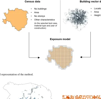
3. The disaggregation is limited to the spatial resolution at which the proxy variable is available. However, this resolution can be suboptimal, especially in the case of hazards with smaller or more narrowly shaped and ir-regular footprints, as explained in the previous section. Thus, when information about buildings is available, namely their locations, footprints and heights, it can provide the grounds for a much more accurate distribution of census val-ues into a finer resolution grid. This procedure can be consid-ered as more than a mere disaggregation, since the building data used actually consist of another layer of information that is integrated. A conceptual representation is shown in Fig. 2. In the present work, the building vector data for the munic-ipality of Pavia, from 2003, were obtained from the Italian Ministry of Environment’s Geoportale Nazionale, through the WFS service (http://wms.pcn.minambiente.it/ogc?map= /msogc/wfs/Edifici.map) (Fig. 3).
construc-Figure 2. Conceptual representation of the method.
Figure 3. Left: building footprints for the municipality of Pavia. Right: highlight of a part of the municipality, with buildings classified by
height, from lower (light orange) to higher (dark orange).
tion (seven). On the other hand, from the data set containing the building locations and geometries, it is only possible to divide the buildings into height classes (number of storeys), since there is no information on the two other variables. In this case, because the material type and age of each individ-ual building are not known, deriving a building-by-building exposure model in a deterministic way is not viable. Thus, a sensible approach is to develop a grid-based exposure model. The fact that actual geographic and geometric building infor-mation is used for disaggregating means that the resolution of the grid can be high, but there are limits past which the results are no longer meaningful, due to the fact that the area distri-butions of some of the required variables are only known at the resolution of the administrative unit. This issue is further discussed in Sect. 3.
The first step in the application of the method consists of assigning height classes, in terms of number of storeys, to different height intervals, in such a way that a correspon-dence can be established between information coming from the census and the vector data sets. The definition of such in-tervals, shown in Table 1, was carried out by combining data on the number of storeys of about 1000 buildings in Pavia, gathered through a field survey, with height information for the same buildings, obtained from Geoportale Nazionale.
Table 1. Correspondence between height classes (census) and
height intervals (building vector data).
No. of storeys Height (m)
1 h≤5.00
2 5.00< h≤8.80 3 8.80< h≤12.30 4 12.30< h≤15.40 5 15.40< h≤19.30 6 19.30< h≤22.00 7 22.00< h≤24.70 8+ h >24.70
Ideally, when developing a residential exposure data set, as in the case of this study, only residential buildings from the vector data set should be considered. However, this is almost always impossible, due to the fact that open data sets con-taining the occupancy type of every building in a region are not commonly available. This does not preclude the applica-tion of the method, since it is mass-preserving in terms of the census areas, meaning that the total areas for the municipal-ity are equal to the sum of the census areas in each grid cell after disaggregation; nevertheless, the better the estimates of V fi andvfi,kare, the more accurate the exposure model is, because of how these variables are used in the process, as presented further below.
In order to improve the accuracy in the estimation of res-idential building footprint areas from vector data without knowledge about the occupancy type of each building indi-vidually, the adopted approach consists of considering all the buildings in the data set except those that fall within certain criteria in terms of area and location. Regarding the former, a footprint area limit of 3200 m2(calibrated using the build-ing data set of Pavia) is defined, above which buildbuild-ings are considered not to be residential. With respect to the latter, CORINE land cover maps (Bossard et al., 2000) are used to exclude buildings located in areas classified as industrial or commercial (Fig. 4).
The estimated floor areas Vi andvi,k, corresponding re-spectively to the footprint areasV fi andvfi,k, are then de-termined by multiplying the footprint areas of each class by the respective number of storeys (s).
Vi=V fi·s (1)
On the side of the census data set, the residential building floor areas for each height classCi0 are calculated by aggre-gating the other census variables, which in this case are the structural material type and the year of construction. Ci0=X
jCi,j (2)
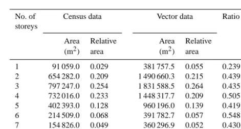
For the present case, the total building floor areas of each height class from both sources are presented in Table 2. It
Figure 4. Municipality of Pavia – building footprints, 1 km2grid and CORINE areas of land cover class “Industrial or commercial units” (in red). Buildings in blue are considered non-residential.
Table 2. Estimated floor areas of the buildings of each height class.
No. of Census data Vector data RatioRi
storeys
Area Relative Area Relative (m2) area (m2) area
1 91 059.0 0.029 381 757.5 0.055 0.239 2 654 282.0 0.209 1 490 660.3 0.215 0.439 3 797 247.0 0.254 1 831 588.5 0.264 0.435 4 732 016.0 0.233 1 448 317.7 0.209 0.505 5 402 393.0 0.128 960 196.0 0.139 0.419 6 214 509.0 0.068 391 782.7 0.057 0.548 7 154 826.0 0.049 360 296.9 0.052 0.430 8+ 88 856.0 0.028 137 878.8 0.020 0.644
the same at municipality level and grid-cell level.
Ri = Ci0
Vi
(3)
ai,k0 =vi,k·Ri (4)
It should also be noted that if a time gap exists between cen-sus and building vector data sets (as in the Pavia case), it can also contribute to the area differences seen in Table 2. However, given the fact that urban structures do not usu-ally change very dynamicusu-ally, its impact is not significant, especially when compared with the other factors mentioned above.
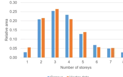
Before proceeding, it is important to check whether the data coming from the two sources – census and vector data sets – are in agreement. This can be done by comparing the distributions of the relative footprint areas of each height class, in relation to the total footprint area of the respective data set. For the municipality of Pavia, the histogram illus-trating those distributions is shown in Fig. 5. The fact that the distributions have similar shapes is a good indicator that the data from both sources are valid and can be confidently used as input for the method. It should be noted that even if there was not such a good agreement between the distributions, the method could still be applied due to its mass-preserving nature, but caution should be exercised in doing so, as that would indicate a likely problem with one or both of the data sets.
The final step of the method consists of disaggregating the building floor areas of each grid cellai,k0 into all the original census classes. In order to do so, it is necessary to calculate, for each height class, the fractions of the areas of the other variables, at municipality level (e.g. fraction of floor area of three-storey masonry buildings built between 1946 and 1961, in relation to the total floor area of three-storey buildings).
Fi,j= Ci,j
Ci0 (5)
Finally, the disaggregated floor areas can be calculated for each grid cell.
ai,j,k=a0i,k·Fi,j (6)
Applying the fractionsFi,j, which are calculated at munic-ipality level, to the grid-cell level, is based on the assumption that for each height class, the distribution of the other vari-ables is similar. The uncertainty introduced by this assump-tion is analysed in Sect. 2.2. In Sect. 3, the impact that it has on the level of spatial resolution up to which the gridded exposure model can be taken is discussed more comprehen-sively.
The method described in this section, which has been coded in Python, is summarized in Fig. 6, in the form of a flowchart.
Figure 5. Comparison of relative building footprint areas of each
height class between census and vector data sets.
2.2 Performance evaluation
As mentioned in the previous subsection, the proposed method was applied in the development of a residential build-ing exposure model for the municipality of Pavia. The per-formance evaluation of the method was carried out using this test case.
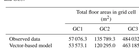
The validation of model results with observed data was performed using a data set provided by the department of territorial planning and management of the municipality of Pavia, containing occupancy types and year of construction classes on a building-by-building basis. Additionally, a sec-ond exposure model based on population distribution was elaborated, with the purpose of comparing results obtained using the two approaches. This model was created by dis-tributing the buildings among the grid cells proportionally to the population, according to the 2011 GEOSTAT population data set. This data set is associated with a 1 km2grid, which was also used for the vector-based model, as well as for ag-gregating the observed building-by-building information, in order to allow a comparison between the three (Fig. 7).
In Fig. 7, three grid cells are highlighted. These cells were selected to illustrate the differences between the two expo-sure models, due to the fact that the existing building typolo-gies in terms of height in each of the cells are considerably different. Grid cell 1 (GC1) corresponds to an area of the municipality with a clear predominance of low-rise buildings (Fig. 8a), while in GC2 the prevailing type of buildings are high-rise (Fig. 8b). Finally, GC3 is located in a more densely populated part of Pavia, in the historical centre of the city.
Figure 6. Flowchart of the method.
Figure 7. The 1 km2 grid adopted in the vector- and population-based exposure models. Grid cells (GC) highlighted in red are used to illustrate the differences between the two models.
The differences between the results obtained in the two ex-posure models are considerable. As expected, the population-based model is unable to capture the distribution of building
Table 3. Total residential building floor areas for cells GC1, GC2
and GC3.
Total floor areas in grid cell (m2)
GC1 GC2 GC3
Observed data 57 076.3 135 789.3 484 032.6
Vector-based model 53 573.1 120 295.0 463 185.9
Population-based model 64 544.2 111 469.2 299 838.3
areas per height class in the different grid cells, as their rel-ative frequencies do not change from municipality level. On the other hand, since the vector-based model takes the build-ing geometries in each cell into account, the shape of the dis-tribution of floor areas per height class is coherent with what can be observed on-site, leading to more accurate results. The total floor areas obtained using the proposed method are also considerably closer to reality, which is particularly evident in the case of GC3.
Figure 8. Bird’s eye images of two areas of the municipality of
Pavia with different predominant building typologies. Top: GC1, mainly low-rise buildings; bottom: GC2, mainly high-rise build-ings. Source: Bing Maps.
directly associated with each other. For this reason, the error introduced by applyingFi,j at grid-cell level, using Eq. (6), needs to be measured separately. In order to do this, we com-pared, at grid-cell level, the real areas with the ones that would be obtained by assuming the fraction distribution at municipality level. Since the data set is compared against it-self, the RMSDs computed in this way reflect that assump-tion individually. The results are shown in Table 5. No data on the material type variable are available, but it is reasonable to assume a similar degree of accuracy.
3 Balance between model resolution and uncertainty The application of the method presented in Sect. 2 enables the possibility of creating grid-based exposure models with a level of spatial resolution that is not constrained by the reso-lution of the input data set, since it consists of actual building footprints instead of gridded information, such as population or land use.
However, given the limited nature of the information that can be obtained from the building data set, the maximum res-olution that the gridded exposure model should have is lim-ited as well. The data set provides locations, footprints and heights of each of the buildings in the municipality, but in-formation on the other variables (in this case, material type
Table 4. Root mean square deviations (RMSDs) of the two models.
Height Population-based Vector-based
class model model
RMSD NRMSD RMSD NRMSD
(m2) (%) (m2) (%)
1 1213.1 16.30 1031.8 13.92
2 9930.0 15.28 6531.8 10.13
3 12 472.7 8.10 4244.4 2.91
4 13 289.1 9.03 5020.3 3.47
5 9349.6 10.06 7389.5 7.99
6 8283.8 11.73 3136.0 4.48
7 5202.2 13.96 1177.1 3.19
8+ 5980.8 12.94 3235.0 7.01
Overall 9021.6 5.86 4517.2 2.93
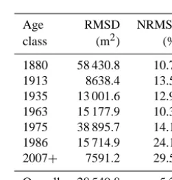
Table 5. Root mean square deviations (RMSDs) of the areas per
grid cell compared with the areas obtained by assuming the fraction distribution at municipality level. NRMSD indicates the normalized RMSD.
Age RMSD NRMSD
class (m2) (%)
1880 58 430.8 10.71
1913 8638.4 13.52
1935 13 001.6 12.99
1963 15 177.9 10.35
1975 38 895.7 14.14
1986 15 714.9 24.19
2007+ 7591.2 29.53
Overall 28 549.8 5.23
and year of construction) is only available at the resolution of the administrative unit. Thus, when performing the spatial disaggregation of census data, the distributions of those vari-ables are kept regardless of the dimensions of the grid cells. This procedure, however, can only be considered valid up to a certain level of spatial resolution of the grid, which corre-sponds to the limit of the assumption of representativeness of the distributions. At higher resolutions, the grid cells become so small and therefore contain so few buildings, that the floor area distributions for each individual cell are meaningless.
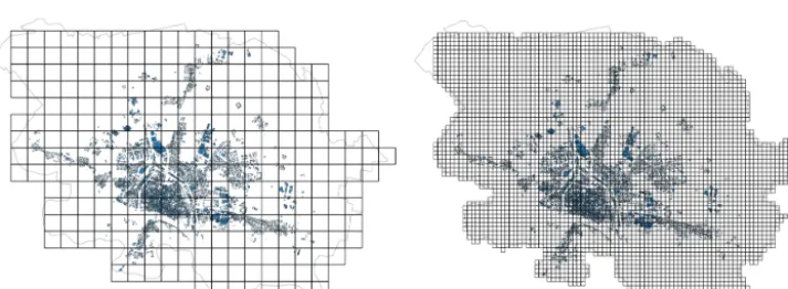
In this section, we analyse the relation between resolution and uncertainty in the development of a gridded exposure model. In order to enable this analysis, the first step con-sisted of generating grids with five different levels of spa-tial resolution, other than the 1 km×1 km grid already shown in the previous section. The selected grid-cell sizes were 750 m×750 m, 500 m×500 m, 250 m×250 m, 125 m×125 m and 50 m×50 m. Two of these grids are shown in Fig. 10.
calcu-Figure 9. Residential building floor areas per height class, from the vector- and population-based exposure models, as well as the observed
data, for three grid cells with different predominant building typologies.
Figure 10. Grids with resolutions of 500 m×500 m (left) and 125 m×125 m (right).
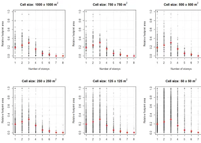
lated in relation to the total residential footprint areas in the same cell. The results are plotted in Fig. 11, together with the census fractions at the level of the municipality.
The coefficient of variation of the root mean square devia-tion (CV(RMSD)) of the relative height class areas, for each grid resolution, was quantified in relation to the relative ar-eas at municipality level. For buildings with one storey and buildings with two storeys, the results are plotted in Fig. 12, together with power law fits to the data. In this figure, it is possible to observe that up to a certain level of resolution, the increase in CV(RMSD) is gradual and relatively constant, after which it becomes more abrupt, between 250 m×250 m and 500 m×500 m. The results are shown for one- and
two-storey buildings as an example; a similar pattern is followed for all the eight height classes.
Figure 11. Relative footprint areas of buildings of each height class in every grid cell, for grids with six different spatial resolutions. Red
rhombuses represent fractions at municipality level.
Figure 12. CV(RMSD) of the relative areas of one-storey (left) and two-storey (right) buildings, for six different levels of resolution of the
grid (50 m×50 m, 125 m×125 m, 250 m×250 m, 500 m×500 m, 750 m×750 m and 1000 m×1000 m), in relation to the relative areas at municipality level, together with power law fits to the data.
that class distributions have similar shapes at municipality and grid-cell levels is no longer reasonable.
If on the one hand, adopting an exposure model with larger grid-cell size results in lower uncertainties in the building class distributions on a cell-by-cell basis, on the other, it can also lead to larger errors when calculating risk, especially in the case of perils with narrowly shaped footprints. Thus, it is paramount to find a good balance between these two aspects.
This issue is further analysed in Sect. 4, for a test case of a flood scenario.
4 Influence of the model resolution on the estimated impacts due to a flood scenario
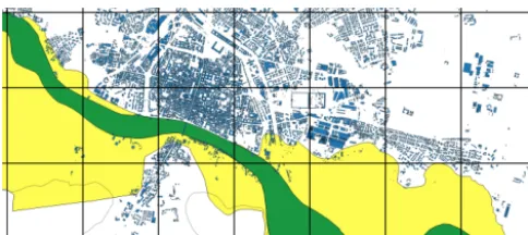
Figure 13. Flood zones A (green) and B (yellow) in the
municipal-ity of Pavia, according to the Po River Basin Authormunicipal-ity map.
a risk model. In order to do so, a straightforward procedure was adopted, based on the estimation of affected floor areas of each building class for a hypothetical flood event in the municipality of Pavia, using different exposure models.
In terms of hazard, the definition of the flood footprint was based on the flood hazard maps produced by the Po River Basin Authority (partially shown in Fig. 13), more specifi-cally flood zone B (fascia B), which covers the areas at risk in case of floods with a return period of 200 years (Autorità di Bacino del fiume Po, 1999). Naturally, this does not mean that a 200-year flood would necessarily affect all the area si-multaneously, but for the purpose at hand, it is reasonable to use it as an estimation of the flood footprint.
Assuming that the water depth of this hypothetical flood is insufficient to reach the second storey of the buildings in the flooded area, the affected floor areas for each of the building classes were calculated, which was done in two steps. Firstly,
ai,j,k was divided by the number of storeys (s), in order to
obtain the ground-level floor areas corresponding to each of the classes. These areas were then multiplied by the fraction of the respective cells covered by the flood footprint (exclud-ing water bodies), which is based on the premise that the as-sets assigned to each grid cell are uniformly distributed in space – an unavoidable procedure when using gridded mod-els. However, that premise is not necessarily true, and this is the fundamental reason why results obtained using grid-ded exposure models with higher spatial resolutions contain smaller errors and are closer to reality, especially when the hazard in question has a narrowly shaped, irregular footprint, as is the case of floods.
The affected areas referred to in the previous paragraph are shown in Table 6 for the six vector-based gridded mod-els mentioned in Sect. 3, as well as for a model based on a uniform spatial distribution of the assets in the munici-pality, without performing any kind of disaggregation. The best estimates of the total affected building areas for this case were also computed, which was done by applying the same method, considering the flood footprint itself as one cell. The relative differences of the results obtained using the aforementioned models with relation to the best estimate are shown as well.
Table 6. Estimated flooded floor areas using different exposure
models.
Model Resolution Affected Ratio
(m2) floor area
(m2)
Best estimate – 29 522.5 –
50×50 31 917.4 1.08
Proposed method 125×125 38 009.6 1.29
at different 250×250 48 018.0 1.63
grid resolutions 500×500 69 506.4 2.35
750×750 90 692.9 3.07
1000×1000 112 085.8 3.80
No disaggregation
(buildings uniformly – 131 797.4 4.46
distributed within municipality)
As shown in Table 6, the estimation of the affected floor areas is highly dependent on the resolution of the adopted exposure model. Using models with lower resolutions led to an overestimation of the areas when compared with the best estimates using the actual flood footprint. These results are coherent with what can be observed by overlapping the flood map, grid and building locations. As it can be observed in Fig. 13, in the majority of cases, buildings are located out-side the parts of the grid cells covered by the flood extension, meaning that the consideration of a uniform spatial distribu-tion of buildings inside each cell tends to lead to an overes-timation of the affected floor areas and, therefore, damages. Understandably, this issue is exacerbated by using a coarser grid, as a higher fraction of cells contain the boundaries of the flood footprint. For other perils, this difference would ex-pectably be lower. When modelling flood events in other ar-eas using a gridded exposure model, a similar behaviour is generally to be expected. This is because usually, buildings tend to be more concentrated outside areas prone to flooding, due to the existence of defences such as levees or as a result of urban planning.
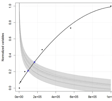
Figure 14. Regression models fitted to the normalized CV(RMSD)
of the eight height classes (grey curves) and estimation errors of affected building areas (black curve).
Conceptually, the obtained regression functions, shown in Fig. 14, are intended to represent the cost of using differ-ent exposure models in relation to their spatial resolution, in terms of accuracy and precision of the building class distribu-tions (represented by the grey curves) and of the errors in the estimation of affected assets (black curve). The lowest total cost – which should correspond to the optimal balance be-tween these two aspects – is given by the intersection of the former with the latter. In this case, its range is represented by blue crosses in Fig. 14.
It should be highlighted that the main purpose behind car-rying out this procedure was to conceptually demonstrate the balance that should exist between the two components, since their costs refer to different types of quantities and the adopted scaling procedure has limitations. The normalization performed in order to bring them into a common range of val-ues is necessary, but ideally they should also be weighted so as to reflect the importance of each of them in the quality of the results of the risk model. This step is outside the scope of the present study, and would be an interesting topic for future research. Nevertheless, the adopted simplified approach can be useful in providing an indication about the range of grid resolutions that can lead to the most reliable results over-all. Following this line of thought, it can be assumed that for the case at hand – as well as in other cases with similar characteristics in terms of hazard and exposure – adopting a gridded model with a resolution between 250 m×250 m and 500 m×500 m would likely ensure a sensible balance between uncertainty in the exposure model and error in the estimation of affected assets.
As a final remark, the discussion presented above is based on the consideration that the exposure model is to be used within a typical risk calculation framework, in which it is de-fined beforehand, with a certain level of resolution and inde-pendently from the spatial characteristics of the hazard. Even though this is the widely adopted procedure for risk calcula-tion, in the case of floods, given the significance of errors that can derive from using coarse exposure models (as shown in Table 6), it is pertinent to suggest and briefly discuss a few potential alternatives, even if they are more complicated and would be more onerous to implement in practical applica-tions. A possible approach would be to use a higher resolu-tion grid that could capture the shape of the hazard more ac-curately, and then reaggregate the results into a coarser grid, so that the number of buildings within each cell would be enough to ensure representativeness of the class distributions and, therefore, the accuracy of the cell-by-cell spatial distri-bution of damages. This procedure, however, could be less practical due to the need to post-process the results. Other potentially interesting approaches would be to develop expo-sure models using variable-resolution grids and/or irregularly shaped cells, defined beforehand by taking the footprints of the hazard maps into account.
5 Conclusions
The building exposure component of risk models is fre-quently based on census data, which is often the most reliable source of building information, but unfortunately is usually only available at coarse resolutions. The disaggregation of census data to a higher resolution grid has often been based on proxies such as the population distribution; this approach, however, is not ideal. In this paper, a method was proposed to take advantage of open building data in order to disaggregate census data in a more sensible way. The building distribu-tions obtained using this method were shown to better cap-ture reality, when compared to models based on population distribution.
Given the incomplete nature of publicly available building information that can generally be obtained, the exposure data set cannot be generated on a building-by-building basis, and thus using a grid is a sensible solution. While the resolution of the grid is not limited to the resolution of a proxy variable, there is another type of limitation related with the fact that only some of the building characteristics are known. After a certain point, the uncertainty in the building distribution at each cell becomes too high and the results are no longer meaningful. This issue was investigated.
case of floods, lower resolutions of the exposure model will in general lead to an overestimation of the affected buildings. A balance should be achieved between, on the one hand, the exposure model’s accuracy and precision, and on other, the errors in the estimation of affected buildings. In order to graphically represent this notion, functions were fitted to each of the components, normalized and intersected; concep-tually, these functions can be understood as cost functions, and in this context, their intersections represent the lowest to-tal costs, which correspond to the optimal resolutions. Even if the procedure was carried out in a simplified manner, it pro-vided a useful indication about the range of grid resolutions to be adopted when applying the proposed method in the de-velopment of exposure data sets for flood risk modelling.
Acknowledgements. This research was supported by the
ECOSTRESS project (Ecological COastal Strategies and Tools for Resilient European SocietieS), funded by the European Commission, DG ECHO (ECHO/SUB/2013/671461).
The authors would also like to acknowledge the department of territorial planning and management of the municipality of Pavia (Settore Pianificazione e Gestione del Territorio, Comune di Pavia) for the data provided.
Edited by: B. Merz
Reviewed by: M. Harb and V. Roezer
References
Autorità di Bacino del fiume Po: Piano stralcio per l’Assetto Idroge-ologico (PAI) – 7.II, Allegato 3 – Metodo di delimitazione delle fasce fluviali, Parma, 1999.
Bing Maps Team: Over 100 New Streetside and 3D
Cities Go Live on Bing Maps (Blog post),
avail-able at: http://blogs.bing.com/maps/2014/08/20/
over-100-new-streetside-and-3d-cities-go-live-on-bing-maps/, last access: 18 March 2015, 2014.
Bossard, M., Feranec, J., and Otahel, J.: CORINE land cover tech-nical guide – Addendum 2000, European Environment Agency, Copenhagen, 2000.
Chen, K., McAneney, J., Blong, R., Leigh, R., Hunter, L., and Mag-ill, C.: Defining area at risk and its effect in catastrophe loss es-timation: a dasymetric mapping approach, Appl. Geogr., 24, 97– 117, doi:10.1016/j.apgeog.2004.03.005, 2004.
Dell’Acqua, F., Gamba, P., and Jaiswal, K.: Spatial aspects of building and population exposure data and their implications for global earthquake exposure modeling, Nat. Hazards, 68, 1291– 1309, doi:10.1007/s11069-012-0241-2, 2012.
Dobson, J. E., Bright, E. A., Coleman, P. R., Durfee, R. C., and Wor-ley, B. A.: LandScan: a global population database for estimat-ing populations at risk, Photogramm. Eng. Rem. S., 66, 849–857, 2000.
Gallego, J. and Peedell, S.: Using CORINE Land Cover to map pop-ulation density, Towards Agri-Environmental Indicators, Topic Report 6/2001, European Environment Agency, Copenhagen, 92–103, 2001.
Gamba, P., Dell’Acqua, F., and Lisini, G.: BREC: the built-up area RECognition tool, in: 2009 Joint Urban Remote Sensing Event, IEEE, 1–5, doi:10.1109/URS.2009.5137593, 2009.
Grossi, P., Kunreuther, H., and Windeler, D.: An introduction to catastrophe models and insurance, in: Catastrophe Modeling: A New Approach to Managing Risk, Springer, USA, 23–42, 2005. Kron, W.: Keynote lecture: Flood risk=hazard×exposure× vul-nerability, in: Flood Defence ’2002, edited by: Wu, B., Wang, Z.-Y., Wang, G., Huang, G. G. H., Fang, H., and Huang, J., Sci-ence Press New York Ltd., 82–97, 2002.
Parikh, B.: Expanded coverage of building footprints in Google Maps (Blog post), available at: http://google-latlong.blogspot. com/2012/10/expanded-coverage-of-building.html, last access: 18 March 2015, 2012.
Silva, V., Crowley, H., Varum, H., and Pinho, R.: Seismic risk as-sessment for mainland Portugal, B. Earthq. Engin., 13, 429–457, doi:10.1007/s10518-014-9630-0, 2014.
Stephenson, D.: Definition, diagnosis and origin of extreme weather and climate events, in: Climate Extremes and Society, Cambridge University Press, New York, 11–23, 2008.
Thieken, A. H., Müller, M., Kleist, L., Seifert, I., Borst, D., and Werner, U.: Regionalisation of asset values for risk analyses, Nat. Hazards Earth Syst. Sci., 6, 167–178, doi:10.5194/nhess-6-167-2006, 2006.
Thieken, A. H., Olschewski, A., Kreibich, H., Kobsch, S., and Merz, B.: Development and evaluation of FLEMOps – a new Flood Loss Estimation MOdel for the private sector, WIT. Trans. Ecol. Envir., 118, 315–324, doi:10.2495/FRIAR080301, 2008. Uden, M. and Zipf, A.: OpenBuildingModels – towards a
plat-form for crowdsourcing virtual 3D cities, in: Progress and New Trends in 3D Geoinformation Sciences, edited by: Pouliot, J., Daniel, S., Hubert, F., and Zamyadi, A., Springer-Verlag, Berlin, doi:10.1007/978-3-642-29793-9, 299–314, 2013.