University of Pennsylvania
ScholarlyCommons
Publicly Accessible Penn Dissertations
2017
Statistical Inference For High-Dimensional Linear
Models
Zijian Guo
University of Pennsylvania, [email protected]
Follow this and additional works at:https://repository.upenn.edu/edissertations
Part of theStatistics and Probability Commons
This paper is posted at ScholarlyCommons.https://repository.upenn.edu/edissertations/2320
For more information, please [email protected].
Recommended Citation
Guo, Zijian, "Statistical Inference For High-Dimensional Linear Models" (2017).Publicly Accessible Penn Dissertations. 2320.
Statistical Inference For High-Dimensional Linear Models
Abstract
High-dimensional linear models play an important role in the analysis of modern data sets. Although the estimation problem has been well understood, there is still a paucity of methods and theories on the inference problem for high-dimensional linear models. This thesis focuses on statistical inference for high-dimensional linear models and consists of the following three parts.
1. The first part of the thesis considers confidence intervals for linear functionals in high-dimensional linear regression. We first establish the convergence rates of the minimax expected length for confidence intervals. Furthermore, we investigate the problem of adaptation to sparsity for the construction of confidence intervals and identify the regimes in which it is possible to construct adaptive confidence intervals.
2. In the second part of the thesis, we consider point and interval estimation of the $\ell_q$ loss of a given estimator in high-dimensional linear regression. For the class of rate-optimal estimators, we establish the minimax rates for estimating their $\ell_{q}$ losses, the minimax expected length of confidence intervals for their $\ell_{q}$ losses and the possibility of adaptivity of confidence intervals for their $\ell_q$ losses.
3. In the third part of the thesis, we consider the problem in the framework of high-dimensional instrumental variable regression and construct confidence intervals for the treatment effect in the presence of possibly invalid instrumental variables. We develop a novel selection procedure, Two-Stage Hard Thresholding (TSHT) to select valid instrumental variables and construct honest confidence intervals for the treatment effect using the selected instrumental variables.
Degree Type
Dissertation
Degree Name
Doctor of Philosophy (PhD)
Graduate Group
Statistics
First Advisor
Tony Cai
Keywords
Accuracy Assessment, Confidence Intervals, High-dimension, Instrumental Variable, Linear Models
Subject Categories
STATISTICAL INFERENCE FOR HIGH-DIMENSIONAL LINEAR MODELS
Zijian Guo
A DISSERTATION
in
Statistics
For the Graduate Group in Managerial Science and Applied Economics
Presented to the Faculties of the University of Pennsylvania
in
Partial Fulfillment of the Requirements for the
Degree of Doctor of Philosophy
2017
Supervisor of Dissertation
T. Tony Cai
Dorothy Silberberg Professor of Statistics
Graduate Group Chairperson
Catherine Schrand
Celia Z. Moh Professor, Professor of Accounting
Dissertation Committee:
Dylan S. Small, Class of 1965 Wharton Professor of Statistics Hongzhe Li, Professor of Biostatistics and Statistics
STATISTICAL INFERENCE FOR HIGH-DIMENSIONAL LINEAR MODELS
COPYRIGHT 2017
Acknowledgments
First and foremost, I would like to express my sincere gratitude to my advisor,
Profes-sor Tony Cai for his strong support during my PhD study. I want to thank Tony for
introducing the thesis topic to me, guiding me through the literature, having
exten-sive discussions with me and giving me full freedom to think through the problems.
I am particularly appreciative to Tony for his great patience and encouragement at
the whole stage of my PhD study. Tony has not just provided academic support, but
also shared his wisdom in both research and life. I could not have imagined having a
better advisor and mentor for my PhD study.
I would also like to thank Professor Dylan Small for motivating me to pursue
PhD in Statistics and supporting me academically and emotionally during both my
undergraduate and PhD study. I met Dylan while I was an undergraduate student
in his applied econometrics course. I am grateful to Dylan for being willing to
su-pervise me when I was a junior student. His encouragement and appreciation of my
undergraduate research motivate me to pursue a PhD in statistics. I want to thank
Dylan for introducing me to causal inference, encouraging me to explore my research
interests and providing support all the time.
being part of my thesis committee. To Hongzhe, thank you for introducing me to the
world of statistical genetics and sharing with me the insights about the connection
between statistics methods and genetics applications. To Zongming, thank you for
teaching me many interesting techniques in your multivariate analysis course.
I would also like to thank Professor Jing Cheng for giving me the opportunity to
be involved with mediation analysis in dental study. I am thankful to Jing and Dylan
for their financial support of five-semester research assistantship.
My special thanks will also go to Hyunseung Kang, Xiaodong Li and Anru Zhang
for helpful discussions and suggestions during my PhD study. To Hyunseung, it is
said that only a few collaborators can write three or more papers together. You are
one of them. To Xiaodong, I really appreciate your sharing your own wisdom in
research. It encourages me to pursue my own research along the right direction. To
Anru, thank you for always sharing your two-year ahead experience with me. It is
fresh and useful.
I would also like to thank all my friends at Penn and other graduates in the
department, whose companion has made my graduate life entertaining and enjoyable.
Special thanks to Anao, Chao, Zhuang, Xin Lu, Sam and Junyang.
Finally, I would like to thank all of my family. Words cannot express my gratitude
for all of your support and love. To my parents, you are my wonderful parents and
wonderful friends. Thank you so much for your unconditional love and constant
support! To Xiaocan, my wife, I am so fortunate to meet you at the beginning of my
PhD study. Thank you for your companion, encouragement, support and love. To
my parents-in-law, thank you for your understanding and support. All of you are my
ABSTRACT
STATISTICAL INFERENCE FOR
HIGH-DIMENSIONAL LINEAR MODELS
Zijian Guo
T. Tony Cai
High-dimensional linear models play an important role in the analysis of modern
data sets. Although the estimation problem has been well understood, there is still a
paucity of methods and theories on the inference problem for high-dimensional linear
models. This thesis focuses on statistical inference for high-dimensional linear models
and consists of the following three parts.
• The first part of the thesis considers confidence intervals for linear functionals
in high-dimensional linear regression. We first establish the convergence rates
of the minimax expected length for confidence intervals. Furthermore, we
inves-tigate the problem of adaptation to sparsity for the construction of confidence
intervals and identify the regimes in which it is possible to construct adaptive
confidence intervals.
• In the second part of the thesis, we consider point and interval estimation of
the `q loss of a given estimator in high-dimensional linear regression. For the
their `q losses, the minimax expected length of confidence intervals for their `q
losses and the possibility of adaptivity of confidence intervals for their`q losses.
• In the third part of the thesis, we consider the problem in the framework of
high-dimensional instrumental variable regression and construct confidence intervals
for the treatment effect in the presence of possibly invalid instrumental variables.
We develop a novel selection procedure, Two-Stage Hard Thresholding (TSHT)
to select valid instrumental variables and construct honest confidence intervals
Contents
1 Introduction 1
1.1 Literature review . . . 1
1.2 Outline of the thesis . . . 2
2 Confidence Intervals for High-Dimensional Linear Regression:
Min-imax Rates and Adaptivity 5
2.1 Introduction . . . 5
2.2 Formulation for adaptive confidence interval problem . . . 10
2.3 Minimax rate and adaptivity of confidence intervals for sparse loading
linear functionals . . . 14
2.4 Minimax rate and adaptivity of confidence intervals for dense loading
linear functionals . . . 21
2.5 Confidence intervals for linear functionals with prior knowledge Ω = I
and σ=σ0 . . . 27
2.6 Discussion . . . 31
2.7 Proofs . . . 32
3.1 Introduction . . . 48
3.2 Minimax estimation of the `q loss . . . 55
3.3 Minimaxity and adaptivity of confidence intervals over Θ0(k) . . . 61
3.4 Minimaxity and adaptivity of confidence intervals over Θ(k) . . . 71
3.5 Estimation of the `q loss of rate-optimal estimators . . . 74
3.6 General tools for minimax lower bounds . . . 76
3.7 An intermediate setting with known σ=σ0 and unknown Σ . . . 80
3.8 Minimax lower bounds for estimating kβk2 q with 1≤q≤2 . . . 82
3.9 Proofs . . . 83
4 Confidence Interval for Causal Effects with Invalid Instruments us-ing Two-Stage Hard Thresholdus-ing 89 4.1 Introduction . . . 89
4.2 Model . . . 93
4.3 Confidence interval estimation via Two-Stage Hard Thresholding . . . 98
4.4 Theoretical results . . . 107
4.5 Simulation . . . 112
4.6 Application: causal effect of years of education on annual earnings . . 116
4.7 Conclusion and discussion . . . 122
A Supplement for Chapter 2 124 A.1 Proofs of Theorems . . . 124
A.2 Proof of lemmas . . . 134
B Supplement for Chapter 3 149 B.1 Difference between Θ(k) and Θ0(k) . . . 149
B.3 Additional lower bound analysis . . . 154
B.4 Upper bound analysis . . . 169
B.5 Proof of extra lemmas . . . 184
C Supplement for Chapter 4 189
C.1 Theory for valid IVs after controlling for high dimensional covariates 189
C.2 Proofs of Theorems . . . 190
C.3 Proof of extra lemmas . . . 201
List of Tables
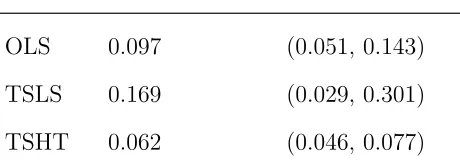
4.1 Estimates of the Effect of Years of Education on Log Earnings. OLS
is ordinary least squares, TSLS is two-stage least squares, and TSHT
List of Figures
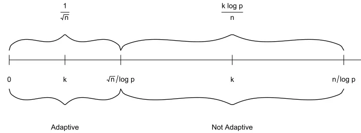
2.1 Illustration of adaptivity of confidence intervals for ξ|β with a sparse
loading ξ satisfying kξk0 ≤ Ck1. For adaptation between Θ(k1) and
Θ(k) with k1 k, rate-optimal adaptation is possible if k .
√
n
logp and
impossible otherwise. . . 19
3.1 The plot demonstrates definitions ofR∗αΘ1,β, `b q
andR∗αΘ1,Θ2,β, `b q
. 63
3.2 Illustration ofR∗αΘ0(k1),βbL, `2
(top) andR∗αΘ0(k1),Θ0(k2),βbL, `2
(bottom)
over regimes k1 ≤ k2 .
√
n
logp (leftmost), k1 .
√
n
logp . k2 . n
logp(middle)
and
√
n
logp .k1 ≤k2 . n
logp (rightmost). . . 66
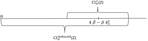
3.3 Comparison of the two-sided confidence interval CI1α(Z) with the
one-sided confidence interval CIinducedα (Z). . . 68
3.4 Illustration ofR∗αΘ (k1),βbSL, `q
(left) andR∗αΘ (k1),Θ (k2),βbSL, `q
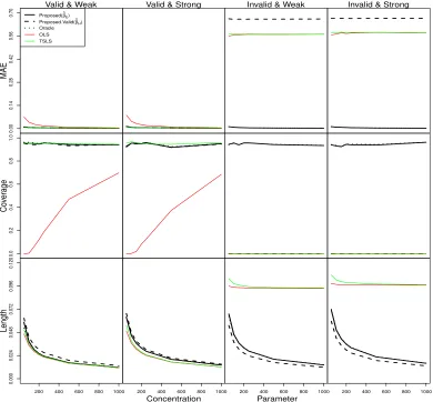
4.1 Comparison of different methods when pz = 100, px = 150 and n = 200.
The x-axis represents the concentration parameter. On the y-axis, MAE represents Median Absolute Error of the estimators, Coverage represents coverage of the confidence intervals and Length represents the average length of confidence intervals. Proposed is our method allowing for invalid IVs and is represented by the solid line. Proposed.valid is our method that assumes all the IVs are valid and is represented by the dashed line. Oracle is the method that knows exactly which instruments are valid and is represented by the dotted line. The column labeled with Valid & Weak represents the case ρ1 = 0.2 and ρ2 = 0. The column labeled with Valid &Strong
represents the case ρ1 = 0 and ρ2 = 0. The column labeled with Invalid
&Weak represents the caseρ1 = 0.2 andρ2= 2. Finally, the column labeled
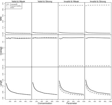
with Invalid & Strong represents the caseρ1 = 0 and ρ2 = 2. . . 117 4.2 Comparison of different methods when pz = 100, px = 150 and n= 1000.
The x-axis represents the concentration parameter. On the y-axis, MAE represents Median Absolute Error of the estimators, Coverage represents coverage of confidence intervals and Length represents the average length of confidence intervals. Proposed is our method allowing for invalid IVs and is represented by the solid line. Proposed.valid is our method that assumes all the IVs are valid and is represented by the dashed line. Oracle is the method that knows exactly which instruments are valid and is represented by the dotted line. The column labeled with Valid & Weak represents the case
ρ1 = 0.2 and ρ2 = 0. The column labeled with Valid &Strong represents
the case ρ1 = 0 and ρ2 = 0. The column labeled with Invalid &Weak
represents the caseρ1 = 0.2 andρ2 = 2. Finally, the column labeled with
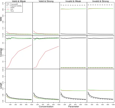
4.3 Comparison of different methods when pz = 9, px = 10 and n = 1000.
The x-axis represents the concentration parameter. On the y-axis, MAE represents Median Absolute Error of the estimators, Coverage represents coverage of confidence intervals and Length represents the average length of confidence intervals. Proposed is our method allowing for invalid IVs and is represented by the solid line. Proposed.valid is our method that assumes all the IVs are valid and is represented by the dashed line. Oracle is the method that knows exactly which instruments are valid and is represented by the dotted line. The column labeled with Valid & Weak represents the case
ρ1 = 0.2 and ρ2 = 0. The column labeled with Valid &Strong represents
the case ρ1 = 0 and ρ2 = 0. The column labeled with Invalid &Weak
represents the caseρ1 = 0.2 andρ2 = 2. Finally, the column labeled with
1
Introduction
1.1
Literature review
Driven by a wide range of applications, the high-dimensional linear model, where the
dimensionpcan be much larger than the sample sizen, has received significant recent
attention. The linear model is
y=Xβ+, ∼N(0, σ2I), (1.1.1)
where y ∈ Rn, X ∈
Rn×p and β ∈Rp. This high-dimensional linear model has been
well studied in the literature, where the main focus has been on estimation of β.
Several penalized/constrained`1 minimization methods, including Lasso (Tibshirani,
1996), Dantzig selector (Cand`es & Tao, 2007), scaled Lasso (Sun & Zhang, 2012)
and square-root Lasso (Belloni et al., 2011), have been proposed. These methods
have been shown to work well in applications and produce interpretable estimates
of β when β is assumed to be sparse. Theoretically, with a properly chosen tuning
parameter, these estimators achieve the optimal rate of convergence over collections
of sparse parameter spaces. See, for example, Cand`es & Tao (2007); Sun & Zhang
van de Geer (2011); Verzelen (2012).
Confidence sets play a fundamental role in statistical inference. Recently,
confi-dence sets for high-dimensional linear models have been actively studied, where the
focus is on the construction of confidence intervals for individual coordinates
(Javan-mard & Montanari, 2014a; van de Geer et al., 2014) and the construction of confidence
balls for the whole high-dimension vectorβ (Nickl & van de Geer, 2013). In addition,
Gautier & Tsybakov (2011); Belloni et al. (2012); Fan & Liao (2014); Chernozhukov
et al. (2015a) provide honest confidence intervals for a treatment effect in the
frame-work of high-dimensional instrumental variable regression. However, compared to the
estimation problem, there is still a paucity of methods and fundamental theoretical
results on the inference problem for high-dimensional linear models. In this thesis,
we will focus on the statistical inference problem in high-dimensional linear models.
An outline of the thesis is presented in the next subsection.
1.2
Outline of the thesis
We consider the following three statistical inference problems in high-dimensional
linear models.
Confidence intervals for linear functionals
In Chapter 2, we consider confidence intervals for linear functionals in high-dimensional
linear regression with random design. We first establish the convergence rates of the
minimax expected length for confidence intervals in the oracle setting where the
spar-sity parameter is given. The focus is then on the problem of adaptation to sparspar-sity
for the construction of confidence intervals. Ideally, an adaptive confidence interval
regres-sion vector, while maintaining a pre-specified coverage probability. It is shown that
such a goal is in general not attainable, except when the sparsity parameter is
re-stricted to a small region over which the confidence intervals have the optimal length
of the usual parametric rate. It is further demonstrated that the lack of adaptivity
is not due to the conservativeness of the minimax framework, but is fundamentally
caused by the difficulty of learning the bias accurately.
This chapter is joint work with T. Tony Cai.
Accuracy assessment
In Chapter 3, we consider point and interval estimation of the `q loss of a given
estimator in high-dimensional linear regression with random design. We establish
the minimax rate for estimating the `q loss and the minimax expected length of
confidence intervals for the`q loss of rate-optimal estimators of the regression vector,
including commonly used estimators such as Lasso, scaled Lasso, square-root Lasso
and Dantzig Selector. Adaptivity of confidence intervals for the`qloss is also studied.
Both the setting of known identity design covariance matrix and known noise level
and the setting of unknown design covariance matrix and unknown noise level are
studied. The results reveal interesting and significant differences between estimating
the `2 loss and `q loss with 1 ≤ q < 2 as well as between the two settings. New
technical tools are developed to establish rate sharp lower bounds for the minimax
estimation error and the expected length of minimax and adaptive confidence intervals
for the `q loss. A significant difference between loss estimation and the traditional
parameter estimation is that for loss estimation the constraint is on the performance
of the estimator of the regression vector, but the lower bounds are on the difficulty
of estimating its `q loss. The technical tools developed in this paper can also be of
This chapter is joint work with T. Tony Cai.
Confidence intervals for treatment effects with invalid
instru-ments
In Chapter 4, we consider the statistical inference problem in the high-dimensional
instrumental variable framework with possibly invalid instruments. The instrumental
variable (IV) method is commonly used to estimate the causal effect of a treatment on
an outcome by using IVs that satisfy the assumptions of association with treatment,
no direct effect on the outcome and ignorability. A major challenge in IV analysis is to
find said IVs, but typically one is unsure of whether all of the putative IVs are in fact
valid (i.e. satisfy the assumptions). We propose a general inference procedure that
provides honest inference in the presence of invalid IVs, even after controlling for a
large number of covariates. The key step of our method is a novel selection procedure,
which we call Two-Stage Hard Thresholding (TSHT), where we use hard thresholding
to select the set of non-redundant instruments in the first stage and subsequently use
hard thresholding to select the set of valid instruments in the second stage among the
set of instruments selected from the first stage. TSHT allows us to not only select
valid IVs, but also provide honest confidence intervals of the treatment effect at √n
rate. We establish asymptotic properties of our procedure and demonstrate that our
procedure performs well in simulation studies compared to traditional IV methods,
especially when the instruments are invalid.
2
Confidence Intervals for High-Dimensional Linear
Regression: Minimax Rates and Adaptivity
2.1
Introduction
Driven by a wide range of applications, high-dimensional linear regression, where the
dimensionpcan be much larger than the sample sizen, has received significant recent
attention. The linear model is
y=Xβ+, ∼N(0, σ2I), (2.1.1)
wherey ∈Rn,X ∈
Rn×p and β ∈Rp. Several penalized/constrained `1 minimization
methods, including Lasso (Tibshirani, 1996), Dantzig Selector (Cand`es & Tao, 2007),
square-root Lasso (Belloni et al., 2011), and scaled Lasso (Sun & Zhang, 2012) have
been proposed and studied. Under regularity conditions on the design matrix X,
these methods with a suitable choice of the tuning parameter have been shown to
achieve the optimal rate of convergence klognp under the squared error loss over the
That is, there exists some constant C >0 such that
sup
kβk0≤k
P
kbβ−βk2 2 > Ck
logp n
=o(1), (2.1.2)
wherekβk0denotes the number of the nonzero coordinates of a vectorβ ∈Rp. See, for
example, Verzelen (2012); Bickel et al. (2009); Cand`es & Tao (2007); Sun & Zhang
(2012). A key feature of the estimation problem is that the optimal rate can be
achieved adaptively with respect to the sparsity parameter k.
Confidence sets play a fundamental role in statistical inference and confidence
in-tervals for high-dimensional linear regression have been actively studied recently with
a focus on inference for individual coordinates. But, compared to point estimation,
there is still a paucity of methods and fundamental theoretical results on confidence
intervals for high-dimensional regression. Zhang & Zhang (2014) was the first to
in-troduce the idea of de-biasing for constructing a valid confidence interval for a single
coordinate βi. The confidence interval is centered at a low-dimensional projection
estimator obtained through bias correction via score vector using the scaled Lasso as
the initial estimator. Javanmard & Montanari (2014a); van de Geer et al. (2014) also
used de-biasing for the construction of confidence intervals and van de Geer et al.
(2014) established asymptotic efficiency for the proposed estimator. All the
afore-mentioned papers, Zhang & Zhang (2014); Javanmard & Montanari (2014a); van de
Geer et al. (2014), have focused on the ultra-sparse case where the sparsity k √
n
logp
is assumed. Under such a sparsity condition, the expected length of the confidence
intervals constructed in Zhang & Zhang (2014); Javanmard & Montanari (2014a);
van de Geer et al. (2014) is at the parametric rate √1
n and the procedures do not
depend on the specific value of k.
Compared to point estimation where the sparsity condition k n
logp is sufficient
for estimation consistency (see equation (2.1.2)), the condition k √
n
confidence intervals is much stronger. There are several natural questions: What
happens in the region where
√
n
logp . k . n
logp? Is it still possible to construct a
valid confidence interval for βi in this case? Can one construct an adaptive honest
confidence interval not depending on k?
The goal of the present paper is to address these and other related questions on
confidence intervals for high-dimensional linear regression with random design. More
specifically, we consider construction of confidence intervals for a linear functional
T (β) = ξ|β, where the loading vector ξ ∈ Rp is given and maxi∈supp(ξ)|ξi|
mini∈supp(ξ)|ξi| ≤ ¯c with
¯
c≥1 being a constant. Based on the sparsity of ξ, we focus on two specific regimes:
the sparse loading regime where kξk0 ≤Ck, with C >0 being a constant; the dense
loading regime where kξk0 satisfying (2.2.7) in Section 2.2. It will be seen later that
for confidence intervals, T (β) = βi is a prototypical case for the general functional
T (β) = ξ|β with a sparse loading ξ, and T (β) = Pp
i=1βi is a representative case for
T (β) = ξ|β with a dense loading ξ.
To illustrate the main idea, let us first focus on the two specific functionals T (β) =
βi and T (β) =Ppi=1βi. We establish the convergence rate of the minimax expected
length for confidence intervals in the oracle setting where the sparsity parameter k is
given. It is shown that in this case the minimax expected length is of order √1
n+k
logp n
for confidence intervals of βi. An honest confidence interval, which depends on the
sparsityk, is constructed and is shown to be minimax rate optimal. To the best of our
knowledge, this is the first construction of confidence intervals in the moderate-sparse
region
√
n
logp k . n
logp. If the sparsityk falls into the ultra-sparse regionk.
√
n
logp, the
constructed confidence interval is similar to the confidence intervals constructed in
Zhang & Zhang (2014); Javanmard & Montanari (2014a); van de Geer et al. (2014).
On the other hand, the convergence rate of the minimax expected length of honest
confidence intervals for Pp
i=1βi in the oracle setting is shown to bek
q
logp
rate-optimal confidence interval that also depends onk is constructed. It should be noted
that this confidence interval is not based on the de-biased estimator.
One drawback of the constructed confidence intervals mentioned above is that
they require a prior knowledge of the sparsityk. Such knowledge of sparsity is usually
unavailable in applications. A natural question is: Without knowing the sparsity k,
is it possible to construct a confidence interval as good as when the sparsity k is
known? This is a question about adaptive inference, which has been a major goal
in nonparametric and high-dimensional statistics. Ideally, an adaptive confidence
interval should have its length automatically adjusted to the true sparsity of the
unknown regression vector, while maintaining a prespecified coverage probability.
We show that, in marked contrast to point estimation, such a goal is in general not
attainable for confidence intervals. In the case of confidence intervals for βi, it is
impossible to adapt between different sparsity levels, except when the sparsity k is
restricted to the ultra-sparse regionk .
√
n
logp, over which the confidence intervals have
the optimal length of the parametric rate √1
n, which does not depend on k. In the
case of confidence intervals for Pp
i=1βi, it is shown that adaptation to the sparsity is
not possible at all, even in the ultra-sparse region k .
√
n
logp.
Minimax theory is often criticized as being too conservative as it focuses on the
worst case performance over a large parameter space. For confidence intervals for
high dimensional linear regression, we establish strong non-adaptivity results which
demonstrate that the lack of adaptivity is not due to the conservativeness of the
min-imax framework. It shows that for any confidence interval with guaranteed coverage
probability over the set of k sparse vectors, its expected length at any given point
in a large subset of the parameter space must be at least of the same order as the
minimax expected length. So the confidence interval must be long at a large subset of
leads directly to the impossibility of adaptation over different sparsity levels.
Funda-mentally, the lack of adaptivity is caused by the difficulty in accurately learning the
bias of any estimator for high-dimensional linear regression.
We now turn to confidence intervals for general linear functionals. For a linear
functionalξ|βin the sparse loading regime, the rate of the minimax expected length is
kξk2
1
√
n+k
logp n
, where kξk2 is the vector`2 norm ofξ. For a linear functionalξ|β
in the dense loading regime, the rate of the minimax expected length iskξk∞k q
logp
n ,
where kξk∞ is the vector `∞ norm of ξ. Regarding adaptivity, the phenomena
ob-served in confidence intervals for the two special linear functionals T (β) = βi and
T (β) = Pp
i=1βi extend to the general linear functionals. The case of confidence
in-tervals for T (β) = Pp
i=1ξiβi with a sparse loading ξ is similar to that of confidence
intervals for βi in the sense that rate-optimal adaptation is impossible except when
the sparsity k is restricted to the ultra-sparse region k .
√
n
logp. On the other hand,
the case for a dense loading ξ is similar to that of confidence intervals for Pp
i=1βi:
adaptation to the sparsity k is not possible at all, even in the ultra-sparse region
k .
√
n
logp.
In addition to the more typical setting in practice where the covariance matrix
Σ of random design and the noise level σ of the linear model are unknown, we also
consider the case with the prior knowledge of Σ = I and σ = σ0. It turns out that
this case is strikingly different. The minimax rate for the expected length in the
sparse loading regime is reduced from kξk2
1
√
n+k
logp n
to k√ξk2
n, and in particular it
does not depend on the sparsity k. Furthermore, in marked contrast to the case of
unknown Σ and σ, adaptation to sparsity is possible over the full range k . n
logp. On
the other hand, for linear functionals ξ|β with a dense loadingξ, the minimax rates
and impossibility for adaptive confidence intervals do not change even with the prior
prior knowledge.
The rest of the paper is organized as follows: After basic notation is introduced,
Section 2.2 presents a precise formulation for the adaptive confidence interval problem.
Section 2.3 establishes the minimaxity and adaptivity results for a general linear
functional ξ|β with a sparse loading ξ. Section 2.4 focuses on confidence intervals
for a general linear functional ξ|β with a dense loading ξ. Section 2.5 considers the
case when there is prior knowledge of covariance matrix of the random design and
the noise level of the linear model. Section 2.6 discusses connections to other work
and further research directions. The proofs of the main results are given in Section
2.7. More discussion and proofs are presented in Chapter A.
2.2
Formulation for adaptive confidence interval
problem
We present in this section the framework for studying the adaptivity of confidence
intervals. We begin with the notation that will be used throughout the paper.
2.2.1
Notation
For a matrix X ∈ Rn×p, X
i·, X·j, and Xi,j denote respectively the i-th row, j-th
column, and (i, j) entry of the matrix X, Xi,−j denotes the i-th row of X excluding
the j-th coordinate, andX−j denotes the submatrix ofX excluding thej-th column.
Let [p] ={1,2,· · · , p}. For a subsetJ ⊂[p],XJ denotes the submatrix ofXconsisting
of columns X·j with j ∈ J and for a vector x ∈ Rp, xJ is the subvector of x with
indices in J and x−J is the subvector with indices in Jc. For a setS, |S|denotes the
cardinality of S. For a vector x ∈ Rp, supp(x) denotes the support of x and the ` q
norm of x is defined as kxkq = (Pqi=1|xi|q)
1
q for q ≥ 0 with kxk
kxk∞= max1≤j≤p|xj|. We use ei to denote the i-th standard basis vector in Rp. For
a ∈ R, a+ = max{a,0}. We use Pβi as a shorthand for Ppi=1βi, maxkX·jk2 as a
shorthand for max1≤j≤pkX·jk2 and minkX·jk2 as a shorthand for min1≤j≤pkX·jk2.
For a matrix A and 1 ≤ q ≤ ∞, kAkq = supkxkq=1kAxkq is the matrix `q operator
norm. In particular, kAk2 is the spectral norm. For a symmetric matrix A, λmin(A)
and λmax(A) denote respectively the smallest and largest eigenvalue of A. We usec
and C to denote generic positive constants that may vary from place to place. For
two positive sequences an and bn, an . bn means an ≤ Cbn for all n and an & bn if
bn .an and an bn if an .bn and bn . an, andan bn if lim supn→∞ abnn = 0 and
an bn if bnan.
2.2.2
Framework for adaptivity of confidence intervals
We shall focus in this paper on the high-dimensional linear model with the Gaussian
design,
yn×1 =Xn×pβp×1+n×1, ∼Nn(0, σ2I), (2.2.1)
where the rows of X satisfy Xi·
i.i.d.
∼ Np(0,Σ), i = 1, ..., n, and are independent of .
Both Σ and the noise levelσ are unknown. Let Ω = Σ−1 denote the precision matrix.
The parameter θ = (β,Ω, σ) consists of the signal β, the precision matrix Ω for the
random design, and the noise level σ. The target of interest is the linear functional
of β, T (β) = ξ|β, where ξ ∈
Rp is a pre-specified loading vector. The data that we
observe is Z = (Z1,· · · , Zn)|, where Zi = (yi, Xi)∈Rp+1 for i= 1,· · ·, n.
For 0 < α < 1 and a given parameter space Θ and the linear functional T (β),
parameter space Θ,
Iα(Θ,T) =
CIα(T, Z) = [l(Z), u(Z)] : inf
θ∈ΘPθ(l(Z)≤T(β)≤u(Z))≥1−α
.
(2.2.2)
For any confidence interval CIα(T, Z) ∈ Iα(Θ,T), the maximum expected length
over a parameter space Θ is defined as
L(CIα(T, Z),Θ,T) = sup
θ∈ΘE
θL(CIα(T, Z)),
where for confidence interval CIα(T, Z) = [l(Z), u(Z)], L(CIα(T, Z)) =u(Z)−l(Z)
denotes its length. For two parameter spaces Θ1 ⊆ Θ, we define the benchmark
L∗α(Θ1,Θ,T) as the infimum of the maximum expected length over Θ1 among all
(1−α)-level confidence intervals over Θ,
L∗α(Θ1,Θ,T) = inf CIα(T,Z)∈Iα(Θ,T)
L(CIα(T, Z),Θ1,T). (2.2.3)
We will write L∗α(Θ,T) for L∗α(Θ,Θ,T), which is the minimax expected length of
confidence intervals over Θ.
We should emphasize that L∗α(Θ1,Θ,T) is an important quantity that measures
the degree of adaptivity over the nested spaces Θ1 ⊂ Θ. A confidence interval
CIα(T, Z) that is (rate-optimally) adaptive over Θ1 and Θ should have the optimal
expected length performance simultaneously over both Θ1 and Θ while maintaining
a given coverage probability over Θ, i.e., CIα(T, Z)∈ Iα(Θ,T) such that
L(CIα(T, Z),Θ1,T)L∗α(Θ1,T) and L(CIα(T, Z),Θ,T)L∗α(Θ,T).
Note that in this case L(CIα(T, Z),Θ1,T) ≥ L∗α(Θ1,Θ,T). So for two parameter
Θ1 and Θ is impossible to achieve.
We consider the following collection of parameter spaces,
Θ(k) =
θ = (β,Ω, σ) :kβk0 ≤k, 1 M1
≤λmin(Ω) ≤λmax(Ω) ≤M1,0< σ≤M2
,
(2.2.4)
where M1 > 1 and M2 > 0 are positive constants. Basically, Θ(k) is the set of all
k-sparse regression vectors. 1
M1 ≤λmin(Ω)≤λmax(Ω)≤M1 and 0< σ≤M2 are two
mild regularity conditions on the design and the noise level.
The main goal of this paper is to address the following two questions:
1. What is the minimax length L∗α(Θ(k),T)in the oracle setting where the sparsity
level k is known?
2. Is it possible to achieve rate-optimal adaptation over different sparsity levels?
More specifically, for k1 k, is it possible to construct a confidence interval
CIα(T, Z) that is adaptive over Θ(k1) and Θ(k) in the sense that CIα(T, Z)∈
Iα(Θ (k),T) and
L(CIα(T, Z),Θ(k1),T)L∗α(Θ(k1),T),
L(CIα(T, Z),Θ(k),T)L∗α(Θ(k),T)?
(2.2.5)
We will answer these questions by analyzing the two benchmark quantitiesL∗α(Θ(k),T)
and L∗α(Θ(k1),Θ(k),T). Both lower and upper bounds will be established. If (2.2.5)
can be achieved, it means that the confidence interval CIα(T, Z) can automatically
adjust its length to the sparsity level of the true regression vector β. On the other
hand, if L∗α(Θ(k1),Θ(k),T)L∗α(Θ(k1),T), then such a goal is not attainable.
For ease of presentation, we calibrate the sparsity level
and restrict the loadingξ to the set
ξ ∈Ξ (q,¯c) =
ξ ∈Rp :kξk
0 =q, ξ 6=0 and
maxj∈supp(ξ)|ξj|
minj∈supp(ξ)|ξj|
≤¯c
,
where ¯c≥1 is a constant. The minimax rate and adaptivity of confidence intervals for
the general linear functionalξ|βalso depends on the sparsity ofξ. We are particularly
interested in the following two regimes:
1. The sparse loading regime: ξ∈Ξ (q,¯c) with
q≤Ck. (2.2.6)
2. The dense loading regime: ξ∈Ξ (q,¯c) with
q =cpγq with 2γ < γ
q ≤1. (2.2.7)
The behavior of the problem is significantly different in these two regimes. We will
consider separately the sparse loading regime in Section 2.3 and the dense loading
regime in Section 2.4.
2.3
Minimax rate and adaptivity of confidence
in-tervals for sparse loading linear functionals
In this section, we establish the rates of convergence for the minimax expected length
of confidence intervals for ξ|β with a sparse loading ξ in the oracle setting where
the sparsity parameter k of the regression vector β is given. Both minimax upper
to be minimax rate-optimal in the sparse loading regime. Finally, we establish the
possibility of adaptivity for the linear functional ξ|β with a sparse loading ξ.
2.3.1
Minimax length of confidence intervals for
ξ
|β
in the
sparse loading regime
In this section, we focus on the sparse loading regime defined in (2.2.6). The following
theorem establishes the minimax rates for the expected length of confidence intervals
for ξ|β in the sparse loading regime.
Theorem 1. Suppose that 0 < α < 1
2 and k ≤ cmin{p
γ, n
logp} for some constants
c >0 and 0≤ γ < 12. If ξ belongs to the sparse loading regime (2.2.6), the minimax
expected length for (1−α) level confidence intervals of ξ|β over Θ (k) satisfies
L∗α(Θ (k), ξ|β) kξk2
1
√
n +k logp
n
. (2.3.1)
Theorem 1 is established in two separate steps.
1. Minimax upper bound: we construct a confidence interval CISα(ξ|β, Z) such
that CISα(ξ|β, Z)∈ I
α(Θ (k), ξ|β) and for some constantC > 0
L CISα(ξ|β, Z),Θ (k), ξ|β
≤Ckξk2
1
√
n +k logp
n
. (2.3.2)
2. Minimax lower bound: we show that for some constant c >0
L∗α(Θ (k), ξ|β)≥ckξk2
1
√
n +k logp
n
. (2.3.3)
The minimax lower bound is implied by the adaptivity result given in Theorem 2.
minimax rate (2.3.1) in the sparse loading regime. The interval CISα(ξ|β, Z) is
cen-tered at a de-biased scaled Lasso estimator, which generalizes the ideas used in Zhang
& Zhang (2014); Javanmard & Montanari (2014a); van de Geer et al. (2014). The
construction of the (random) length is different from the aforementioned papers as
the asymptotic normality result is not valid once k&
√
n
logp.
Let {β,b ˆσ} be the scaled Lasso estimator with λ0 = q
2.05 logp
n ,
{β,b σˆ}= arg min
β∈Rp,σ∈
R+
ky−Xβk2 2 2nσ +
σ 2 +λ0
p
X
j=1
kX·jk2
√
n |βj|. (2.3.4)
Define
b
u= arg min
u∈Rp
n
u|Σbu:kbΣu−ξk∞≤λn
o
, (2.3.5)
whereΣ =b n1X|X andλn= 12kξk2M12 q
logp
n . The confidence interval CI S
α(ξ|β, Z) is
centered at the following de-biased estimator
e
µ=ξ|βb+ b
u|1 nX
|y−X
b
β, (2.3.6)
whereβbis the scaled Lasso estimator given in (2.3.4) andbuis defined in (2.3.5). Before
specifying the length of the confidence interval, we review the following definition of
restricted eigenvalue introduced in Bickel et al. (2009),
κ(X, k, α0) = min
J0⊂{1,···,p},
|J0|≤k
min
δ6=0,
kδJ c
0k1≤α0kδJ0k1
kXδk2
√
nkδJ0k2
. (2.3.7)
Define
ρ1(k) =kξk2σˆmin
1.01
s
b
u|Σb
b
u nkξk2 2
zα/2+C1(X, k)k logp
n , logp( 1
√
n +
klogp n )
,
where zα/2 is the α/2 upper quantile of the standard normal distribution and
C1(X, k) = 7000M12
√
n minkX·jk2
max
1.25, 912 maxkX·jk 2 2
nκ2X, k,405maxkX·jk2
minkX·jk2
. (2.3.9)
Define the event
A={σˆ ≤logp}. (2.3.10)
The confidence interval CISα(ξ|β, Z) for ξ|β is defined as
CISα(ξ|β, Z) =
[µe−ρ1(k), µe+ρ1(k)] onA
{0} onAc
(2.3.11)
It will be shown in Section 2.7 that the confidence interval CISα(ξ|β, Z) has the desired
coverage property and achieves the minimax length in (2.3.1).
Remark 1. In the special case ofξ =e1, the confidence interval defined in (2.3.11) is
similar to the ones based on the de-biased estimators introduced in Zhang & Zhang
(2014); Javanmard & Montanari (2014a); van de Geer et al. (2014). The second
term ub|1
nX|
y−Xβb
in (2.3.6) is incorporated to reduce the bias of the scaled
Lasso estimator βb. The constrained estimator b
u defined in (2.3.5) is a score vector u
such that the variance term u|Σbu is minimized and one component of the bias term
kbΣu−ξk∞ is constrained by the tuning parameter λn. The tuning parameter λn is
chosen as 12kξk2M12
q
logp
n such thatu= Ωξlies in the constraint setkbΣu−ξk∞≤λn
in (2.3.5) with overwhelming probability. For C1(X, k) defined in (2.3.9), it will be
2.3.2
Adaptivity of confidence intervals for
ξ
|β
in the sparse
loading regime
We have constructed a minimax rate-optimal confidence interval forξ|β in the oracle
setting where the sparsity k is assumed to be known. A major drawback of the
construction is that it requires prior knowledge of k, which is typically unavailable
in practice. An interesting question is whether it is possible to construct adaptive
confidence intervals that have the guaranteed coverage and automatically adjust its
length to k.
We now consider the adaptivity of the confidence intervals for ξ|β. In light of
the minimax expected length given in Theorem 1, the following theorem provides an
answer to the adaptivity question (2.2.5) for the confidence intervals for ξ|β in the
sparse loading regime.
Theorem 2. Suppose that 0 < α < 12 and k1 ≤ k ≤ cmin
n
pγ, n
logp
o
for some
constants c >0and 0≤γ < 12. If ξ belongs to the sparse loading regime (2.2.6), then
there is some constant c1 >0 such that
L∗α(Θ(k1),Θ(k), ξ|β)≥c1kξk2
1
√
n +k logp
n
. (2.3.12)
Note that Theorem 2 implies the minimax lower bound in Theorem 1 by taking
k1 = k. Theorem 2 rules out the possibility of rate-optimal adaptive confidence
intervals beyond the ultra-sparse region. Consider the setting where k1 k and
√
n
logp k . n
logp. In this case,
L∗α(Θ(k1),Θ(k), ξ|β)L∗α(Θ(k), ξ|β) kξk2k logp
n L
∗
α(Θ(k1), ξ|β).
over Θ(k1) and Θ(k) when
√
n
logp k . n
logp and k1 k. For sparse loading with
q ≤ Ck1, the only possible region for adaptation is the ultra-sparse region k .
√
n
logp,
over which the optimal expected length of confidence intervals is of order √1
n and in
particular does not depend on the specific sparsity level. These facts are illustrated
in Figure 2.1.
1
n
k log p
n
0 k n log p k n log p
Adaptive Not Adaptive
Figure 2.1: Illustration of adaptivity of confidence intervals for ξ|β with a sparse
loading ξ satisfying kξk0 ≤ Ck1. For adaptation between Θ(k1) and Θ(k) with k1 k, rate-optimal adaptation is possible if k.
√
n
logp and impossible otherwise.
So far the analysis is carried out within the minimax framework where the focus
is on the performance in the worst case over a large parameter space. The minimax
theory is often criticized as being too conservative. In the following, we establish
a stronger version of the non-adaptivity result which demonstrates that the lack of
adaptivity for confidence intervals is not due to the conservativeness of the minimax
framework. The result shows that for any confidence interval CIα(ξ|β, Z), under the
coverage constraint that CIα(ξ|β, Z) ∈ Iα(Θ (k), ξ|β), its expected length at any
given θ∗ = (β∗,I, σ)∈Θ (k1) must be of order kξk2
1
√
n+k
logp n
. So the confidence
interval must be long at a large subset of points in the parameter space, not just at
a small number of “unlucky” points.
Theorem 3. Suppose that 0 < α < 12 and k ≤ cmin{pγ, n
logp} for some constants
0 < ζ0 < 1. Then for any θ∗ = (β∗,I, σ) ∈ Θ (k1) and ξ ∈ Ξ (q,¯c), there is some
constant c1 >0 such that
inf
CIα(ξ|β,Z)∈Iα(Θ(k),ξ|β)
Eθ∗L(CIα(ξ|β, Z))≥c1kξk2
klogp
n +
1
√
n
σ. (2.3.13)
Note that no supremum is taken over the parameter θ∗ in (2.3.13). Theorem 3
illustrates that if a confidence interval CIα(ξ|β, Z) is “superefficient” at any point
θ∗ = (β∗,I, σ)∈Θ(k1) in the sense that
Eθ∗L(CIα(ξ|β, Z)) kξk2
1
√
n +k logp
n
σ,
then the confidence interval CIα(ξ|β, Z) can not have the guaranteed coverage over
the parameter space Θ(k).
2.3.3
Minimax rate and adaptivity of confidence intervals for
β
1We now turn to the special case T (β) = βi, which has been the focus of several
previous papers, Zhang & Zhang (2014); Javanmard & Montanari (2014b,a); van de
Geer et al. (2014). Without loss of generality, we consider β1, the first coordinate
of β, in the following discussion and the results for any other coordinate βi are the
same. The linear functionalβ1 is the special case of linear functional of sparse loading
regime with ξ=e1.
Theorem 1 implies that the minimax expected length for (1−α) level confidence
intervals of β1 over Θ (k) satisfies
L∗α(Θ (k), β1) 1
√
n +k logp
In the ultra-sparse region withk .
√
n
logp, the minimax expected length is of order
1
√
n.
However, when k falls in the moderate-sparse region
√
n
logp k . n
logp, the minimax
expected length is of order klognp and in this case klognp √1
n. Hence the confidence
intervals constructed in Zhang & Zhang (2014); Javanmard & Montanari (2014b,a);
van de Geer et al. (2014), which are of parametric length √1
n, asymptotically have
coverage probability going to 0. The condition k .
√
n
logp is thus necessary for the
parametric rate √1
n. van de Geer et al. (2014) established asymptotic normality
and asymptotic efficiency for a de-biased estimator under the sparsity assumption
k
√
n
logp. Similar results have also been given in Ren et al. (2013) for a related
problem of estimating a single entry of a p-dimensional precision matrix based on n
i.i.d. samples under the same sparsity condition k √
n
logp. It was also shown that
k √
n
logp is necessary for the asymptotic normality and asymptotic efficiency results.
The following corollary, as a special case of Theorem 3, illustrates the strong
non-adaptivity for confidence intervals of β1 when k
√
n
logp.
Corollary 1. Suppose that 0 < α < 12 and k ≤ cmin{pγ,lognp} for some constants
c >0 and 0≤γ < 1
2. Let k1 ≤(1−ζ0)k−1for some constant 0< ζ0 <1. Then for
any θ∗ = (β∗,I, σ)∈Θ (k1), there is some constant c1 >0 such that
inf
CIα(β1,Z)∈Iα(Θ(k),β1)
Eθ∗L(CIα(β1, Z))≥c1
1
√
n +k logp
n
σ. (2.3.15)
2.4
Minimax rate and adaptivity of confidence
in-tervals for dense loading linear functionals
We now turn to the setting where the loading ξ is dense in the sense of (2.2.7).
We will also briefly discuss the special casePp
i=1βi and the computationally feasible
2.4.1
Minimax length of confidence intervals for
ξ
|β
in the
dense loading regime
The following theorem establishes the minimax length of confidence intervals of ξ|β
in the dense loading regime (2.2.7).
Theorem 4. Suppose that 0 < α < 12 and k ≤ cmin{pγ, n
logp} for some constants
c > 0 and 0≤ γ < 12. If ξ belongs to the dense loading regime (2.2.7), the minimax
expected length for (1−α) level confidence intervals of ξ|β over Θ (k) satisfies
L∗α(Θ (k), ξ|β) kξk∞k r
logp
n . (2.4.1)
Note that the minimax rate in (2.4.1) is significantly different from the minimax
ratekξk2(√1n+klognp) for the sparse loading case given in Theorem 1. In the following,
we construct a confidence interval CIDα (ξ|β, Z) achieving the minimax rate (2.4.1) in
the dense loading regime. Define
C2(X, k) = 822
√
n minkX·jk2
max
1.25, 912 maxkX·jk 2 2
nκ2X, k,405maxkX·jk2
minkX·jk2
. (2.4.2)
It will be shown that C2(X, k) is upper bounded by a constant with overwhelming
probability. The confidence interval CIDα (ξ|β, Z) is defined to be,
CIDα (ξ|β, Z) =
h
ξ|βb− kξk∞ρ2(k), ξ|βb+kξk∞ρ2(k)
i
onA
{0} onAc
(2.4.3)
where A is defined in (2.3.10) and βb is the scaled Lasso estimator defined in (2.3.4)
and
ρ2(k) = min
(
C2(X, k)k
r
logp
n σ,ˆ logp k
r
logp n σˆ
!)
The confidence interval constructed in (2.4.3) will be shown to have the desired
cover-age property and achieve the minimax length in (2.4.1). A major difference between
the construction of CIDα (ξ|β, Z) and that of CIS
α(ξ|β, Z) is that CI D
α (ξ|β, Z) is not
centered at a de-biased estimator. If a de-biased estimator is used for the construction
of confidence intervals for ξ|β with a dense loading, its variance would be too large,
which leads to a confidence interval with length much larger than the optimal length
kξk∞k q
logp
n .
2.4.2
Adaptivity of confidence intervals for
ξ
|β
in the dense
loading regime
In this section, we investigate the possibility of adaptive confidence intervals for ξ|β
in the dense loading regime. The following theorem leads directly to an answer to
the adaptivity question (2.2.5) for confidence intervals for ξ|β in the dense loading
regime.
Theorem 5. Suppose that 0 < α < 12 and k1 ≤ k ≤ cmin
n
pγ,lognp
o
for some
constants c >0 and 0≤γ < 1
2. If ξ belongs to the dense loading regime (2.2.7), then
there is some constant c1 >0 such that
L∗α(Θ (k1),Θ (k), ξ|β)≥c1kξk∞k r
logp
n . (2.4.5)
Theorem 5 implies the minimax lower bound in Theorem 4 by taking k1 =k. If
k1 k, (2.4.5) implies
L∗α(Θ (k1),Θ (k), ξ|β)≥ckξk∞k r
logp
n L
∗
α(Θ (k1), ξ|β), (2.4.6)
is not possible at all for any k1 k. In contrast, in the case of the sparse loading
regime, Theorem 2 shows that it is possible to construct an adaptive confidence
interval in the ultra-sparse regionk.
√
n
logp, although adaptation is not possible in the
moderate-sparse region
√
n
logp k. n
logp.
Similarly to Theorem 3, the following theorem establishes the strong non-adaptivity
results for ξ|β in the dense loading regime.
Theorem 6. Suppose that 0 < α < 12 and k ≤ cmin{pγ,lognp} for some constants
c >0 and 0≤ γ < 1
2. Let q satisfy (2.2.7) and k1 ≤(1−ζ0)k−1 for some positive
constant 0 < ζ0 < 1. Then for any θ∗ = (β∗,I, σ) ∈ Θ (k1) and ξ ∈ Ξ (q,¯c), there is
some constant c1 >0 such that
inf
CIα(ξ|β,Z)∈Iα(Θ(k),ξ|β)E
θ∗L(CIα(ξ|β, Z))≥c1kξk∞k
r
logp
n σ. (2.4.7)
2.4.3
Minimax length and adaptivity of confidence intervals
for
P
pi=1
β
iWe now turn to to the special case of T(β) = Pp
i=1βi, the sum of all regression
coefficients. Theorem 4 implies that the minimax expected length for (1−α) level
confidence intervals of Pp
i=1βi over Θ (k) satisfies
L∗αΘ (k),Xβi
k
r
logp
n . (2.4.8)
The following impossibility of adaptivity result for confidence intervals forPp
i=1βi is
a special case of Theorem 6.
Corollary 2. Suppose that 0 < α < 12 and k ≤ cmin{pγ, n
logp} for some constants
any θ∗ = (β∗,I, σ)∈Θ (k1),
inf
CIα(Pβi,Z)∈Iα(Θ(k),Pβi)
Eθ∗L
CIα
X
βi, Z
≥c1k
r
logp
n σ, (2.4.9)
for some constant c1 >0.
Remark 2. In the Gaussian sequence model, minimax estimation of the sum of
sparse means has been considered in Cai & Low (2004) and construction of confidence
intervals for the sum was studied in Cai & Low (2005). In particular, minimax
estimation rate and minimax expected length of confidence intervals are given in Cai
& Low (2004) and Cai & Low (2005), respectively. A more refined non-asymptotic
analysis for the minimax estimation of the sum of sparse means was given in a recent
paper Collier et al. (2015).
2.4.4
Computationally feasible confidence intervals
A major drawback of the minimax rate-optimal confidence intervals CISα(ξ|β, Z) given
in (2.3.11) and CIDα (ξ|β, Z) given in (2.4.3) is that they are not computationally
fea-sible as both depend on restricted eigenvalueκ(X, k, α0), which is difficult to evaluate.
In this section, we assume the prior knowledge of the sparsity k and discuss how to
construct a computationally feasible confidence interval.
The main idea is to replace the term involved with restricted eigenvalue by a
computationally feasible lower bound function ω(Ω, X, k) defined by
ω(Ω, X, k) =
1 4pλmax(Ω)
−
91 + 405maxkX·jk2
minkX·jk2
p
λmin(Ω)
r
klogp n
2
+
. (2.4.10)
The lower bound relation is established by Lemma 13 in Chapter A, which is based on
λmin(Ω) andλmax(Ω), all terms in (2.4.10) are based on the data (X, y) and the prior
knowledge of k. To construct a data-dependent computationally feasible confidence
interval, we make the following assumption,
sup Ω∈GΩ
PX
maxn
λ^min(Ω)−λmin(Ω) ,
λmax^(Ω)−λmax(Ω) o
≥Can,p
=o(1),
(2.4.11)
where lim supan,p = 0 andGΩ is a pre-specified parameter space for Ω andPX denotes
the probability distribution with respect to X.
Remark 3. We assume GΩ is a subspace of the precision matrix defined in (2.2.4),
n
Ω : M1
1 ≤λmin(Ω)≤λmax(Ω) ≤M1
o
. By assuming GΩ is the set of precision
ma-trix of special structure, we can find estimators satisfying (2.4.11). For example,
if GΩ is assumed to be the set of sparse precision matrices, the precision matrix Ω
can be estimated by the CLIME estimator Ω proposed in Cai et al. (2011). Un-e
der a proper sparsity assumption on Ω, the plugin estimator λ^min(Ω),λmax^(Ω)
=
λmin
e
Ω, λmax
e
Ω satisfies (2.4.11). Other special structures can also be
as-sumed, for example, the covariance matrix Σ is sparse. We can use the plugin
es-timator of the thresholding eses-timators proposed in Cai & Liu (2011); Cai & Zhou
(2012).
With λ^min(Ω) and λmax^(Ω), we defineωe(Ω, X, k) as
e
ω(Ω, X, k) =
1
4
q
^ λmax(Ω)
−
91 + 405maxkX·jk2
minkX·jk2
q
^ λmin(Ω)
r
klogp n
2
+ .
and construct computationally feasible confidence intervals by replacing
κ2
X, k,405
maxkX·jk2 minkX·jk2
in (2.3.11) and (2.4.3) with eω(Ω, X, k).
2.5
Confidence intervals for linear functionals with
prior knowledge
Ω = I
and
σ
=
σ
0We have so far focused on the setting where both the precision matrix Ω and the noise
level σ are unknown, which is the case in most statistical applications. It is still of
theoretical interest to study the problem when Ω and σ are known. It is interesting
to contrast the results with the ones when Ω and σ are unknown. In this case, we
consider the setting where it is known a priori that Ω = I and σ=σ0 and specify the
parameter space as
Θ(k,I, σ0) ={θ = (β,I, σ0) :kβk0 ≤k}. (2.5.1)
We will discuss separately the minimax rates and adaptivity of confidence intervals
for the linear functionals in the sparse loading regime and dense loading regime over
the parameter space Θ(k,I, σ0).
2.5.1
Confidence intervals for linear functionals in the sparse
loading regime
The following theorem establishes the minimax rate of confidence intervals for linear
functionals in the sparse loading regime when there is prior knowledge that Ω = I
and σ =σ0.
Theorem 7. Suppose that 0 < α < 12 and k ≤ cmin{pγ, n
logp} for some constants
expected length for (1−α) level confidence intervals of ξ|β over Θ(k,I, σ
0) satisfies
L∗α(Θ(k,I, σ0), ξ|β)
k√ξk2
n . (2.5.2)
Compared with the minimax rate k√ξk2
n +kξk2k
logp
n for the unknown Ω and σ case
given in Theorem 1, the minimax rate in (2.5.2) is significantly different. With the
prior knowledge of Ω = I and σ = σ0, the above theorem shows that the minimax
expected length of confidence intervals for ξ|β is always of the parametric rate and
in particular does not depend on the sparsity parameter k. In this case, adaptive
confidence intervals for ξ|β is possible over the full range k ≤c n
logp. A similar result
for confidence intervals covering all βi was given in a recent paper Javanmard &
Montanari (2015). The focus of Javanmard & Montanari (2015) is on individual
coordinates, not general linear functionals.
The proof of Theorem 7 involves establishment of both minimax lower and upper
bounds. The lower bound follows from the same proof for the parametric lower
bound in Theorem 1. As both Ω and σ are known, the upper bound analysis is
easier than the unknown Ω and σ case and is similar to the one given in Javanmard
& Montanari (2015). For completeness, we detail the construction of a confidence
interval achieving the minimax length in (2.5.2) using the de-biasing method. We
first randomly split the samples (X, y) into two subsamples X(1), y(1)
and X(2), y(2)
with sample sizes n1 andn2, respectively. Without loss of generality, we assume that
n is even and n1 = n2 = n2. Let βbdenote the Lasso estimator defined based on the
sample X(1), y(1)
with the proper tuning parameter λ=
q
2.05 logp
n1 σ0,
b
β = arg min
β∈Rp
ky(1)−X(1)βk2 2 2n1
+λ
p
X
j=1
kX·(1)j k2
√
n1
We define the following estimator ofξ|β,
¯
µ=ξ|βb+
1 n2
ξ| X(2)|y(2)−X(2)βb
. (2.5.4)
Based on the estimator, we construct the following confidence interval
CIIα(ξ|β, Z) =
¯
µ−1.01k√ξk2
n2
zα0/2σ0, µ¯+ 1.01
kξk2
√
n2
zα0/2σ0
, (2.5.5)
where α0 =γ0α with 0< γ0 <1. It will be shown in Chapter A that the confidence
interval proposed in (2.5.5) has the nominal coverage probability asymptotically and
achieves the minimax length in (2.5.2).
2.5.2
Confidence intervals for linear functionals in the dense
loading regime
The following theorem establishes the adaptivity lower bound in the dense loading
regime.
Theorem 8. Suppose that 0 < α < 12 and k1 ≤ k ≤ cmin
n
pγ,lognpo for some
constants c >0 and 0≤γ < 12. If ξ belongs to the dense loading regime (2.2.7), then
there is some constant c1 >0 such that
L∗α(Θ (k1,I, σ0),Θ (k,I, σ0), ξ|β)
≥ c1kξk∞σ0max
(
p
kk1
r
logp n ,min
(
k
r
logp n ,
√
k
n14
))
. (2.5.6)
Remark 4. There are two parts in the lower bound given in (2.5.6), which are
estab-lished separately. The lower bound min
k
q
logp
n ,
√
k
n14
is obtained using well known
techniques by testing a simple null against a composite alternative. The construction
favorable set has been used under the Gaussian sequence model in Baraud (2002) for
signal detection and in Cai & Low (2004, 2005) for estimation and confidence
inter-vals for linear functionals. The technique has also been used more recently in Ingster
et al. (2010); Nickl & van de Geer (2013) for detection and confidence ball in sparse
linear regression. On the other hand, the other lower bound, √kk1
q
logp
n , cannot be
established using a similar argument and a novel comparison of two composite least
favorable spaces is introduced to establish this lower bound.
The lower bound given in (2.5.6) immediately yields the minimax lower bound for
the expected length of confidence intervals over Θ (k,I, σ0),
L∗α(Θ (k,I, σ0), ξ|β)≥c1kξk∞k r
logp n σ0,
by simply setting k1 = k in (2.5.6). Since this lower bound can be achieved by the
confidence interval constructed in (2.4.3), we have established the minimax
conver-gence rate L∗α(Θ (k1,I, σ0), ξ|β) kξk∞k q
logp
n σ0, which is the same as the minimax
rate established in Theorem 4 for the case of unknown Ω and σ. Thus, in marked
contrast to the sparse loading regime, the prior knowledge of Ω = I and σ =σ0 does
not improve the minimax rate in the dense loading regime. Under the framework
(2.2.5), adaptive confidence intervals are still impossible, since for k1 k,
L∗α(Θ (k1,I, σ0),Θ (k,I, σ0), ξ|β)L∗α(Θ (k1,I, σ0), ξ|β).
However, compared with Theorem 5, we observe that the cost of adaptation is reduced