R E G U L A R A R T I C L E
Open Access
Complex network analysis of teaching
practices
Woon Peng Goh
1,2*, Dennis Kwek
3, David Hogan
4and Siew Ann Cheong
2,5*Correspondence:
1Interdisciplinary Graduate School,
Nanyang Technological University, 50 Nanyang Avenue, Singapore, 639798, Singapore
Full list of author information is available at the end of the article
Abstract
The application of functional analysis to infer networks in large datasets is potentially helpful to experimenters in various fields. In this paper, we develop a technique to construct networks of statistically significant transitions between variable pairs from a high-dimensional and multiscale dataset of teaching practices observed in Grade 5 and Grade 9 Mathematics classes obtained by the National Institute of Education in Singapore. From the Minimum Spanning Trees (MST) and Planar Maximally Filtered Graphs (PMFG) of the transition networks, we establish that teaching knowledge as truth and teacher-dominated talking serve as hubs for teaching practices in Singapore. These practices reflect a transmissionist model of teaching and learning. We also identify complex teacher-student-teacher-student interaction sequences of teaching practices that are over-represented in the data.
Keywords: complex networks; functional analysis; teaching practices; pedagogy
theory
1 Introduction
In recent years, it has become popular to use networks to visualize and analyze the hi-erarchical structure within large datasets usually obtained from complex dynamical sys-tems. Networks are especially useful for representing the extent and magnitude of inter-actions among the many components in complex systems. In such visualizations we show the important pair-wise relationships between variables. These relations may be directed transitions, causation, or activations, or undirected when we examine similarities or co-occurrences. Examples of such usage can be found in finance [, ], biology [, ], sociology [], and language []. Even without any further quantitative analysis of the network struc-ture, showing such pair-wise relationships on a network often gives us a powerful overview of the structures that exist within the data. Beyond such crude ‘eyeballing’ of the network, there exist tools to (i) filter out the most essential structure in the network [–], (ii) iden-tify important central nodes, (iii) quaniden-tify the hierarchical structure [, ], (iv) ideniden-tify important patterns or paths in the network [], and (v) identify clusters of nodes [, ]. Broadly speaking, there are two approaches to generate networks from data. First, some datasets such as air traffic data [, ] and World Wide Web connectivity data [] contain explicit information about the network structure. In other cases, we often have to infer the interactions among various components or variables by performing functional analysis on the data []. Examples of this approach include the estimation of an undirected network of
stocks based on the Pearson correlations of their daily returns [], as well as the mapping of a directed functional network of brain regions from fMRI data using Granger causality as a directed measure []. In both examples, the resulting network provides us deeper insights into the system it represents - clustering of stocks in similar industries in the stock market, and a functional hierarchy in the brain. We believe there is great potential in applying functional analysis to infer networks in large datasets under-utilized by experimenters in various fields.
In , the National Institute of Education (NIE) conducted a large-scale study of teach-ing practices in Steach-ingapore classrooms drawteach-ing on a representative national sample of schools. The study had the goal of investigating how teachers teach in Singapore, why they teach the way they do, and the effects of their teaching on student learning. The overall focus of the study was to map and model the logic of pedagogical instruction, the intel-lectual quality of knowledge work in classrooms, and the impact of instructional practice on student achievement while controlling for student and family characteristics. A total of English and Mathematics lessons from Grades and classes were video-recorded and manually annotated for the presence of some instructional indicators over the course of each lesson. These indicators focus on a broad range of organisational, instruc-tional and interacinstruc-tional practices in the classroom, the knowledge and cognitive focus of teaching, the types of classroom talk and their knowledge content, how students respond, and the quality of the disciplinary knowledge of the subject-domain (English and Math-ematics). The resulting data set is extremely high-dimensional (one dimension for each indicator) with greatly varying activities - some indicators are present up to % of the time while others appear only .% of the time. Using commercial software such as SPSS to analyse the large dataset proved to be computationally intensive, as it explores the combinatorially large space of variables to find statistically significant transitions. In particular, such commercial software was unable to perform complex temporal analysis of classroom pedagogy, which remains a major methodological challenge for educational research [].
we illustrate what the method is capable of discovering only for the data of Grade and Grade Mathematics.
2 Data
The data used in our analysis was obtained by the National Institute of Education through a comprehensive, large-scale, multi-dimensional, baseline study of descriptive and obser-vational data on the state of instructional practices in Singapore classrooms. Known as the Core Research Programme, it was a collaborative effort conducted by a team of over research professors, research assistants and associates, and postdoctoral fellows and led by Professor David Hogan []. The Core Programme utilized a nested design compris-ing three distinct, inter-related, and analytical lines of research, each designated a ‘Panel’ with specific foci ranging from teacher and student beliefs, attitudes, and motivations (using surveys), classroom instructional practices (using videographic observations and coding), and assessment practices (using artefactual analysis). The anonymized data used for this paper is drawn from the observational and coding panel which videotaped and collected data from English and Mathematics teachers in Primary schools and Sec-ondary schools. Grades (in Primary schools) and (in SecSec-ondary schools) were selected as these were considered to be years crucial to the development of skills and knowledge needed for the high stakes national examinations for Primary schools (the Singapore Pri-mary School Leaving Examination) and Secondary schools (the General Cambridge ‘O’ Level Examination). English and Mathematics were selected as key curriculum areas that have a significant influence on student social mobility; literacy and numeracy skills are of-ten seen as key leverages to opening up educational and career pathways. Data were col-lected from April through November , resulting in lessons (with - lessons per subject-level combination). Teachers selected for observation were asked to nominate a unit of work - a full sequence of lessons around a particular topic, theme or content area. Rather than discrete, random lessons for observation, the stipulation of a unit of work fa-cilitates subsequent analyses that charts, models, and examines the developmental ebb and flow of knowledge and skills over time.
the lesson with a short summary statement of what was taught for that lesson. Students would then rise, bow and thank the teacher for the lesson.
All lessons are video and audio recorded using two to three high-definition video cam-eras and up to four audio recorders, with the aim to capture all whole class interactions and the majority of pair or group work. Lesson recordings are then coded by subject spe-cialists who are intensively trained in the use of the Singapore Pedagogy Coding Scheme [, ]. Video recorded lessons, unlike in-situ classroom coding, afforded the detailed refinement of the coding scheme with the possibility of recoding to resolve any coding errors. Coded data are entered into Microsoft Excel and compiled in SPSS for statistical analyses. Each lesson is coded in three-minute ‘phases’, with an average one hour lesson having phases. In each phase, the states of more than possible listed variables (we use variables as a more general term for instructional practices) are coded through man-ual annotation. See Additional file for detailed descriptions of the variables as well as the decision to code in three-minute phases. Segmenting the lesson into phases allows for a temporal examination of instructional practices from the start to the end of a lesson, and across the unit of work. From these variables, we selected roughly which are believed to be most essential to the development of the intellectual quality of knowledge work for our network analysis.
The variables chosen extends current pedagogical research based on John Hattie’s re-search on ‘Visible Learning’ which describes effective pedagogical practices [], by fo-cusing on the nature of students doing disciplinary knowledge work in the classroom: the epistemic focus of instructional tasks; the nature of knowledge practices (including the generation, representation, communication and justification of knowledge claims); the epistemic classroom talk that helps makes these knowledge claims explicit, transparent and visible to students; and the cognitive complexity of the knowledge work undertaken in instructional tasks, recognising the contested nature of knowledge claims []. These selected variables are coded as either active () or inactive () for each lesson phase.
3 Methods
3.1 Defining transitions
The starting point of our analysis is to define what constitutes a transition from one vari-able to another and from this, develop a measure of transition frequency and significance. Previous work in network analysis tended to use measures like conditional probability [], transfer entropy [, ], or Pearson correlation [] to denote the relationship be-tween variable pairs. The major shortcoming in these measures when applied to discrete binary signals is that they do not consider the characteristic event durations, i.e. a signal that is activated continuously across several phases are assumed to be distinct events at each phase and treated independently.
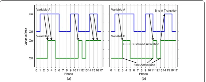
To formulate our definition of a transition from variableito variablej, we assume: (i) the dynamics of the variables in our data set are well approximated by a lag- Markov process i.e. the states of the variables at phaset+ are solely conditioned on their states at phaset
(see Figure (a) and (b)), and (ii) when a variable is active from phasettot+l, but not present att– , it is regarded as a single self-sustaining process first activated at phaset
and lasting for durationl(see Figure (c)). For assumption (i) Figure (a) demonstrates that for a majority of variables, the ability to determine whether or not they are active at phase
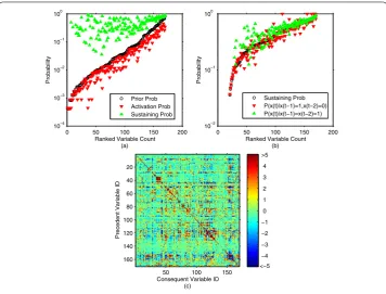
Figure 1 Comparison of Markov probabilities and colour map of correlations.In(a), the open circles are the prior probabilitiesPi(the probability of observing an active variableiat a given phase), the upwards
pointing triangles are sustaining probabilitiesP(xi(t) = 1|xi(t– 1) = 1) (the probability of observing an activei
given thatiis already active at a preceding phase), and the downwards pointing triangles are the first activation probabilitiesP(xi(t) = 1|xi(t– 1) = 0) (the probability of observing an activeigiven thatiinactive at a
preceding phase). We ranked the variables in increasing order of prior probabilities. We see clearly that a vast majority of the sustaining probabilities are at least an order of magnitude larger than their corresponding prior probabilities. These variables have the tendency to self-sustain which suggests that we should treat multiple-phase activation of these variables as a single event. In(b)we compare the lag-1 sustaining probabilities against the probabilitiesP(xi(t) = 1|xi(t– 1) = 1,xi(t– 2) = 0) andP(xi(t) = 1|xi(t– 1) = 1,xi(t– 2) = 1)
(i.e. treating variables as a lag-2 dynamical process). Unlike in(a), there is no clear increase in probability when the second preceding phase is accounted for. In(c)we show, on a colour map, the standard scores of observed conditional probabilitiesPobserved(xj(t) = 1|xi(t– 1) = 1) against their expected values ifiandjwere
independent. Ifiandjwere independent and characterized solely by their respective prior probabilitiesPi
andPj, the expected conditional probabilities should be equal to the prior, i.e.
Pexpected(xj(t) = 1|xi(t– 1) = 1) =Pjand the distribution of conditional probabilities should have a standard
deviation ofσ=Pj(1 –Pj)/Ni. The standard score is obtained fromZ= (Pobserved(xj(t) = 1|xi(t– 1) = 1) –Pj)/σ.
The colours on the map range from blue (lower than expected) to teal (equals expectation), and finally maroon (higher than expected). The dominant feature of this map is a diagonal of higher-than-expected conditional probabilities for self-transitions.
variables att– . We also see from Figure (b) that the additional knowledge of their state att– , however, did not improve significantly our prediction capability. Thus, the lag- Markov process is sufficient and also efficient in modelling the dynamics of the variables in our data set. In Figure (c), we showed that for a variable iwhich is active fromtto
t+l, it is much more likely that the active state att+kwhere ≤k≤lis a self-transition fromt+k– tot+krather than it being triggered by an external variable (assumption (ii)). Therefore, we search for inter-variable transitions only at the instances of first activations. A transition is thus defined as an event whereby a consequent variable has been triggered (or first activated) by the activity of the precedent. Formally, we say a transition fromitoj
Figure 2 Method of counting transitions.If we count all active state to active state transitions between variable pairs as shown in(a), there will be 5 transitions from variableAtoB. This method assumes that every phase in which a variable is active is independent of its previous phase(s). If we assume that variables are activated in blocks, i.e. first activated at a particular time and then self-sustained for a duration, then it becomes reasonable to count transition frequencies as shown in(b). In(b), transitions always result in a variable’s first activation. We count twoAtoBtransitions and oneBtoAtransition.
j(t) = ). The total number of transitions from variableitojis therefore
N(j←i) =
L
l=
Tl–
t=
xli(t) –xlj(t)xlj(t+ ) ()
wherexlj(t) is the state of variablejat phasetof lessonl,Lis the total number of lessons for a particular subject-level combination andTlis the number of phases in lessonl. The
procedure is illustrated in Figure .
3.2 Measuring significance
For two variables that are frequently active, the number of mutual first activations will also be large, even if they are causally unrelated. On the other hand, for two variables that are rarely active, even a small number of first activations may indicate strong causal relation between them if this number is larger than expected by chance. To test a transition frequency for statistical significance, we use the Monte Carlo sampling method described below.
Given a pair of variablesiandjthat we assume are uncorrelated, we can create synthetic signals of each variable with their lag- Markov models using the Monte Carlo sampling scheme explained in Table . This is our null model for the observed transitions fromi
toj. We generatedk= , synthetic signalsxˆl
i,h(t),h= , . . . ,kfor variablei, andxˆlj,h(t),
h= , . . . ,kfor variablejand computed the total number of transitionsNˆh,h= , . . . ,kas
described in Equation () for each pair. The population ofktransition frequencies form a distribution ofNˆ.
Letpbe the fraction of the population ofNˆ that is larger than or equal to the observed number of transitionsNobserved(j←i). Ifp≈ thenNobservedis far above the mean of this distribution, there is a far greater number of observed transitions fromitojthan expected from the null model which assumed the variablesiandjwere independent. Ifp≈. then
Nobservedis close to the median of this distribution, and can be well explained by the null
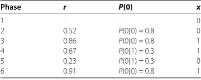
Table 1 Monte Carlo sampling example
Phase r P(0) x
1 – – 0
2 0.52 P(0|0) = 0.8 0
3 0.86 P(0|0) = 0.8 1
4 0.67 P(0|1) = 0.3 1
5 0.23 P(0|1) = 0.3 0
6 0.91 P(0|0) = 0.8 1
SupposeP(0|0) = 0.8,P(1|0) = 1 –P(0|0) = 0.2,P(0|1) = 0.3,P(1|1) = 1 –P(0|1) = 0.7, and we start withx(1) = 0. Then to generate a sequence using these transition probabilities, we draw 5 random numbersr= (0.52, 0.86, 0.67, 0.23, 0.91)uniformly from the interval[0, 1)and allowx(t) = 0whenr<P(0|0),x(t– 1) = 0andx(t) = 0whenr<P(0|1),x(t– 1) = 1. Sincex(1) = 0, to obtainx(2)we look atP(0|0). Since
r(2) <P(0|0),x(2) = 0. However,r(3) >P(0|0), givingx(3) = 1. Iterating further, sincex(3) = 1, we look atP(0|1)andr(4) >P(0|1),x(4) = 1. Thenr(5) <P(0|1),x(5) = 0. Finally,r(6) >P(0|0), andx(6) = 1. The sequence we get is thereforex= (0, 0, 1, 1, 0, 1).
We take the significance value to bes= – p. By rescaling in this manner,s≈, , or – if the observed transition frequencyNobservedis, respectively, approximately the same as, greater than, or less than the value expect from the null model. We can then compute the significance-weighted transition frequencies by multiplying each transition frequency with its significance. The weighting procedure diminishes insignificant frequencies and makes lower-than-expected frequencies negative. The weighted scores are
Nweighted(i←j) =sN(i←j). ()
For our analysis, we admit only edges where the significances> ., i.e.p< . and thus there is %confidence that the transition is not spurious.
3.3 Network visualization and filtering
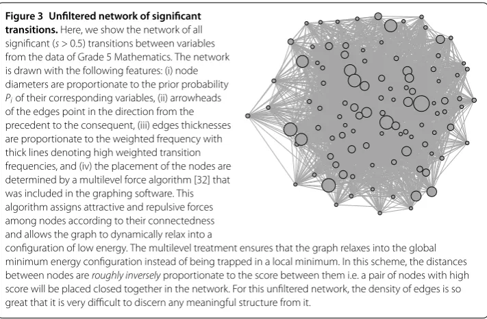
We then visualize the weighted transition frequenciesNweightedon two complex directed networks (one for Grade Mathematics and one for Grade Mathematics) where each node on the network represents a variable and the directed edges between nodes denote transitions. If we show all the edges in these networks without any filtering, we get ‘fur balls’ like that shown in Figure . The network is too densely interconnected and the im-portant structures are obscured. Therefore it is essential to apply filtering schemes that remove less important edges and highlight the more important ones. We employ two pop-ular techniques widely used in complex network analysis. They are the Minimal Spanning Tree (MST) [] and the Planar Maximally Filtered Graph (PMFG) []. Since we seek to identify transitional motifs (paths) in this work, it is important to choose a method that preserves connectedness. We selected the MST and PMFG filtering methods because they guarantee connectedness in the resulting network (at least in the undirected sense). Other popular complex network filtering schemes, such as threshold filtering and disparity fil-tering [] do not satisfy this condition
Figure 3 Unfiltered network of significant transitions.Here, we show the network of all significant (s> 0.5) transitions between variables from the data of Grade 5 Mathematics. The network is drawn with the following features: (i) node diameters are proportionate to the prior probability
Piof their corresponding variables, (ii) arrowheads
of the edges point in the direction from the precedent to the consequent, (iii) edges thicknesses are proportionate to the weighted frequency with thick lines denoting high weighted transition frequencies, and (iv) the placement of the nodes are determined by a multilevel force algorithm [32] that was included in the graphing software. This algorithm assigns attractive and repulsive forces among nodes according to their connectedness and allows the graph to dynamically relax into a
configuration of low energy. The multilevel treatment ensures that the graph relaxes into the global minimum energy configuration instead of being trapped in a local minimum. In this scheme, the distances between nodes areroughly inverselyproportionate to the score between them i.e. a pair of nodes with high score will be placed closed together in the network. For this unfiltered network, the density of edges is so great that it is very difficult to discern any meaningful structure from it.
Figure 4 Construction of MST and PMFG graphs. The solid lines in(a)show a MST graph built from decreasing order of edge weights i.e. the edges with the highest weights are included first. The edges represented by dashed lines with weights 8, 4, and 1 are not included since they will result in loops in the network.(b),(c), and(d)shows the properties of the PMFG. Even though the edges in(b)intersect, the graph is planar. This is because the lines can easily be redrawn such that they do not intersect like in (c). However, if the new blue edge is added to the graph(d)there is no way to redraw the edges or rearrange the nodes such that the links never intersect. Therefore the graph in(d)is not planar.
The PMFG filtering scheme, similar to the MST, admits edges in decreasing order of strength starting from the strongest link as long as the graph remains planar. Without elaborating on mathematical details, a planar graph is a graph that can in principle be em-bedded on a planar surface without any crossing of links (see Figure (b)-(d)). The PMFG retains more information ((N– ) links) while conserving all the hierarchical structure associated with the MST.
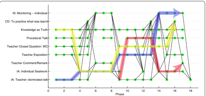
Figure 5 Time-resolved transition chart.The time-resolved chart of a limited set for variables for a chosen lesson. Diagonal lines in the chart represent significant (s> 0.5) transitions defined in Section 3.1. There are several paths in the chart which involves two or more transitions (three or more variables) and some of these paths are highlighted. For each path on the time-resolved chart there is a corresponding path in the time-integrated transition network.
3.4 Dynamical motifs
Beyond recognizing just the pairwise transitions between lesson variables, we also wish to identify important sequences of two or more significant transitions which we call dynam-ical motifs. These sequences enables us to track the progression of practices across many phases spanning a longer duration of a lesson. To do so, we return to the annotated data of individual lessons and search for frequently occurring sequences of significant transitions. This procedure is illustrated in a form of a time-resolved chart shown in Figure . Dynam-ical motifs identified are sequences that were repeated frequently over many lessons.
4 Results
4.1 Prevalent transitions in teaching practices
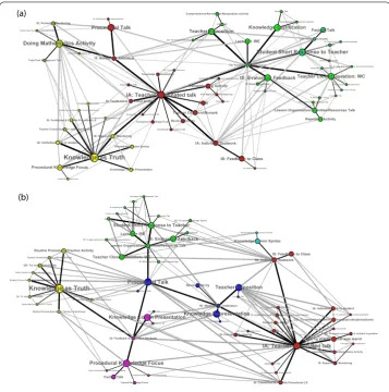
In Figures (a) and (b), the filtered graphs of weighted transition frequencies are shown for Grade Mathematics and Grade Mathematics respectively. We can observe that across both grade levels, teaching practices are organised around source (outgoing) hubs that correspond to Knowledge as Truthand Instructional Activity (IA): Teacher-Dominated Talk. These source hubs are characterized by a large concentration of sig-nificant outgoing transitions. Although these hubs also tend to be the most frequent prac-tices, the frequency alone does not account for the large number of significant outgoing transitions. This suggests strongly thatKnowledge as TruthandInstructional Activity (IA): Teacher-Dominated Talkare indeed important hubs that drive the initiation of teaching sequences.
Figure 6 Transition networks of teaching practices during Mathematics lessons.The PMFG-filtered networks for(a)Grade 5 Mathematics and(b)Grade 9 Mathematics are drawn with features (i), (ii), and (iii) as described in Figure 3. We use dark edges to highlight the MST backbone of the PMFG network. The node placement was determined by the same multilevel force algorithm [32] in Figure 3 acted on the MST edges. We also indicate the community of the nodes in the graph by their colour. They are detected with a community-detection algorithm [13] that was built into the graphing software based on its MST backbone as well. The detection process, not guided by any pedagogy theory, nevertheless produced communities of variables that are in general agreement in pedagogy theory.
“well done”, etc.). But whileDoing Mathematics Activityis a generative node in Grade , it all but disappears by Grade (Figure (b)). We also note the presence of sink (incoming) hubs such asCD: To Practice What Was Learnt,IA: Individual Seatwork, andIS: Monitor-ing - Individualwhich attracts several significant incoming transitions. Unlike the source hubs, sink hubs are practices that occur much less frequently and are harder to detect. The network analysis methodology uniquely discerns these hubs with their special role.
Here, we find that whileIA: Individual SeatworkandIS: Monitoring - Individualremain as prominent sink hubs for Grade ,IS: Feedback to Individual Studentshas replacedCD: To Practice What Was Learntin its role.
4.2 Motifs of teaching practices
The most common length- and length- motifs for Grade and Grade Mathematics are shown in Figure . A motif is said to be length-nif it consists ofn– successive sig-nificant transitions, but is not followed by annth transition that is statistically significant. Some of the length- motifs contain a length- stem that branches out into more than one statistically significant fourth transition.
As we can see, Grade motifs typically show a common ‘cycle’ of teaching: The teacher starts talking about content (IA: Teacher-Dominated Talk,Knowledge as Truth, Procedu-ral Talk); next, students are often given individual practice work (IA: Individual Seat-work); then, the teacher provides some feedback (Comment/Remark), returns to lengthy talk (IA: Teacher-Dominated Talk,Exposition), or asks the whole class a closed question which typically has one correct answer (Teacher Closed Question: WC). Sometimes, the sequences carry on with more practice work (CD: To Practice What Was Learnt,IA: In-dividual Seatwork) as well as the teacher’s monitoring of the student learning (IS: Mon-itoring - Individual,IS: Formative Monitoring,IS: Supervisory Monitoring) or providing individual feedback (IS: Feedback to Individual Students,IA: Individual Talk to Student). The Grade motifs are largely similar to those in Grade , but with a greater focus on
Procedural Knowledge Focusin the middle of the common motifs. Also, some Grade lessons tend to end with the teacher providing a closing exposition (Teacher Exposition), lecture, and IRE (a form of talk where the teacher Initiates, the student Responds, and the teacher Evaluates) (Lecture,Lecture+IRE).
Interestingly, there are motif links such asIA: Individual SeatworktoTeacher Exposi-tionfor Grade ,Procedural TalktoIA: Individual Seatworkfor Grade , andProcedural Knowledge FocustoIS: Monitoring - Individualfor Grade which are present in the collec-tion of common motifs in Figure while not appearing in their respective PMFG-filtered networks in Figure . The PMFG filtering scheme picks edges in descending order of statis-tical significance. However, because the statisstatis-tical significances are time-integrated, there is no guarantee that successive transitions in the PMFG appear one after the other during actual lessons. These time-integrated transitions may be part of two motifs, one ending at the node that the other starts at. This is why a time-resolved analysis must also be carried out to identify dynamical motifs consisting of successive transitions that are statistically significant.
5 Discussion
that goes on inside students’ minds as knowledge is transferred or transmitted from the teacher to the student; simpler facts and procedures should be learned first, followed by progressively more complex facts and procedures; the way to determine the success of schooling is to test students to see how many of these facts and procedures they have acquired through well-established assessment procedures. In the transition networks of both Grade and Grade Mathematics,Knowledge as TruthandInstructional Activity (IA): Teacher-Dominated Talkare seen as dominant hubs.Knowledge as Truthmeans that the knowledge that is presented in the lesson is viewed as non-contestable, non-negotiable and objectively valid. As anInstructional Activity (IA),Teacher-Dominated Talkmeans simply that the teacher does most of the talking in the classroom. These practices operate most effectively in the transmissionist model of teaching, since knowledge is unproblem-atic and non-contestable, and teachers need only to ensure that they cover the curricu-lum. Not the least of the opportunity costs forTeacher-Dominated Talkhowever, is that when students are not given the opportunity to engage in extended and productive discus-sions during lessons, misconceptions often go undetected, existing conceptual schemas can go unchallenged, students might become disengaged with the learning process, and over time, because they have less agency in the class to speak up, and lose motivation to become good students.
However, as Ball [] points out, mathematics instruction ought to involve a lot more than the transmission of facts and procedures. Above all, mathematics instruction should provide students with rich opportunities to engage in authentic, domain-specific mathe-matical practices. “Mathematics practices,” she goes on, “focus on the mathemathe-matical know-how, beyond content knowledge, that constitutes expertise in learning and using math-ematics [such as] justifying claims, using symbolic notation efficiently, defining terms precisely, and making generalisations are examples of mathematical practices.” Thus, the transmissionist model is insufficient as a teaching and learning model for mathematics. In Grade , the strong presence ofDoing Mathematics Activityis an important practice that we hoped to see in mathematics classrooms.Doing Mathematics Activityis inher-ently disciplinary in nature, and students need to acquire the mathematics-specific dis-ciplinary skills, knowledge and disposition to understand mathematics deeply, debate, and discuss mathematical procedures and concepts, and appreciate the importance and relevance of mathematics. It captures the idea that mathematics learning does not con-sist purely of learning algorithmic procedures (captured inProcedural Talk and Proce-dural Knowledge Focus) and content (captured in Factual TalkandFactual Knowledge Focus), but requires students to perform discipline-specific knowledge practices as out-lined by Ball. Similarly, Stein and Lane [] characterize ‘doing mathematics’ as “The use of complex, non-algorithmic thinking to solve a task in which there is not a predictable, well-rehearsed approach or pathway explicitly suggested by the task, task instructions, or a worked out example. ‘Doing mathematics’ processes are often likened to the pro-cesses in which mathematicians engage when solving problems.” These activities are the most demanding of all activities, since they require the students to draw upon a range of mathematical knowledge and procedures/skills to complete some work that has no well-rehearsed way of completing the task. Instead, students are likely to be asked to design, test and justify a new procedure to fit a new kind of problem.
understand-ing of mathematics has been replaced by a focus on procedural knowledge (Procedural Knowledge Focus) as an effective and efficient means to present such knowledge, such as efficient problem solving methods. Yet, we believe that it is precisely because of this peda-gogical approach focused on a highly proceduralised and efficient form of learning abstract mathematics that has made Singapore one of the top performing countries in international assessments that measure students’ ability in mathematics. Our observation confirms the PISA findings on Singapore Mathematics [] which shows that there is a strong relationship between the teaching of Formal Mathematics (as opposed to Applied Math-ematics or Word Problems) and student mathematical performance in the PISA tests.
Finally, teaching and learning must be understood as a process. Christie [] talks of the prototypical classroom lesson having a beginning, middle and end pattern. The begin-ning comprises some form of teacher direction (Curriculum Initiation), followed by the teacher and students’ sharing of direction (Curriculum Collaboration/Negotiation) and ending with students’ independent activity (Curriculum Closure). In the motifs we iden-tified for Grade and Grade , the didactic of student-teacher as well as teacher-student-teacher-student sequences highlights the complex interaction cycles that occur in mathematics classrooms. Almost all lessons begin, as described above, with a teacher-led initiation (Knowledge as Truth,Instructional Activity (IA): Teacher-Dominated Talk,
Procedural Talk,Procedural Knowledge Focus). Often, these motifs lead immediately to individual practice work (IA: Individual Seatwork), seemingly replacing the middle phase of Christie’s pattern with student’s independent activity. Some motifs then terminate with feedback from the teacher in the form of lengthy talk (Teacher Comment/Remark,IA: Teacher-Dominated Talk, Teacher Exposition) following student’s practice work. These motifs suggest a teacher-dominated closure in the teaching pattern. However, in other motifs, we discovered a fourth movement which is a return to more practice work (CD: To Practice What Was Learnt) coupled with teacher’s monitoring of such practice work (IS: Monitoring - Individual,IS: Formative Monitoring,IS: Supervisory Monitoring).
In Grade , the greater focus onProcedural Knowledge Focusis in line with the high stakes environment that Grade teachers and students are entrenched in, requiring stu-dents to learn - at least a year early from the Grade national examinations - procedures and practice skills that are necessary to perform well in the high stakes mathematics ex-amination. Interestingly, when the focus is onProcedural Knowledge Focus, it is often fol-lowed by a more personalised approach where the teacher may provide individualised, specific, feedback (IS: Feedback to Individual Students) or learning support (IS: Contex-tual & Flexible Procedural LS). Such feedback and support are positive signs that rather than a summative exposition at the end (which does occur nevertheless), teachers and stu-dents have the opportunity to provide some feedback to one another. Expositions do end in about half of the motifs, likely due to the need to ensure that the important content and skills are reiterated and summarised, a necessary conclusion to the transmissionist model.
6 Conclusion
of several practices and activities that are common in many lessons. We established that teaching practices of both Grade and Grade Mathematics lessons are organized around
Knowledge as TruthandInstructional Activity (IA): Teacher-Dominated Talkhubs which exemplify the transmissionist model of teaching. In addition, aDoing Mathematics Activ-ityhub is present in the Grade transition network. This suggests that teaching practices at this level have incorporated exploratory elements into the pedagogy, a positive sign to-wards the goal of st century learning. In contrast, in Grade , disciplinary understanding of mathematics has been replaced by a focus on procedural knowledge, which nevertheless accounts for Singapore’s strong performance in international benchmarks. The motifs we extracted from the network highlight cycles of complex teacher-student-teacher-student sequences with great similarity between Grade and Grade . In future work, this method-ology will be employed and modified for more in-depth study of the transitions data. This includes using knowledge of the topology of the transition network to formulate strategies that can direct the flow of teaching activities towards a desired outcome.
Additional material
Additional file 1: Singapore Pedagogy Coding Scheme 2
Competing interests
The authors declare that they have no competing interests.
Authors’ contributions
DH and DK provided the functionally coded data set, and the pedagogical conceptual framework for this study. They also jointly framed and interpreted the results of the data analysis. SAC and WPG developed the complex transitions network methodologies and tests for statistical significances, while WPG performed the data analysis. WPG, DK, SAC were principally responsible for writing the manuscript while DH reviewed and rewrote sections of the penultimate draft of the manuscript.
Author details
1Interdisciplinary Graduate School, Nanyang Technological University, 50 Nanyang Avenue, Singapore, 639798,
Singapore. 2Complexity Institute, Nanyang Technological University, 60 Nanyang View, Singapore, 639673, Singapore. 3Office of Education Research, National Institute of Education, 1 Nanyang Walk, Singapore, 637616, Singapore.4School of
Education, Faculty of Humanities and Social Sciences, University of Queensland, Brisbane, QLD 4072, Australia.5School of Physical & Mathematical Sciences, Nanyang Technological University, 21 Nanyang Link, Singapore, 637371, Singapore.
Acknowledgements
The data is drawn from a National Institute of Education project OER 20/09DH, Core 2 Research Programme (Panel 3), funded by the Office of Education Research, National Institute of Education. The project’s principal investigator is Professor David Hogan, and the co-principal investigators are Dr Phillip Towndrow and Dr Dennis Kwek. Data were collected and coded by over 15 research assistants and associates, led by Professor David Hogan, Dr Phillip Towndrow, Dr Dennis Kwek, and Dr Ridzuan Rahim.
Received: 31 July 2014 Accepted: 10 December 2014
References
1. Mantegna RN (1999) Hierarchical structure in financial markets. Eur Phys J B 11(1):193-197
2. Tumminello M, Lillo F, Mantegna RN (2010) Correlation, hierarchies, and networks in financial markets. J Econ Behav Organ 75(1):40-58
3. Jeong H, Mason SP, Barabási A-L, Oltvai ZN (2001) Lethality and centrality in protein networks. Nature 411(6833):41-42 4. Milo R, Shen-Orr S, Itzkovitz S, Kashtan N, Chklovskii D, Alon U (2002) Network motifs: simple building blocks of
complex networks. Science 298(5594):824-827
5. Potterat JJ, Phillips-Plummer L, Muth SQ, Rothenberg RB, Woodhouse DE, Maldonado-Long TS, Zimmerman HP, Muth JB (2002) Risk network structure in the early epidemic phase of HIV transmission in Colorado Springs. Sex Transm Infect 78(Suppl 1):i159-i163
6. Solé RV, Corominas-Murtra B, Valverde S, Steels L (2010) Language networks: their structure, function, and evolution. Complexity 15(6):20-26
7. Tumminello M, Aste T, Di Matteo T, Mantegna RN (2005) A tool for filtering information in complex systems. Proc Natl Acad Sci USA 102(30):10421-10426
9. Radicchi F, Ramasco JJ, Fortunato S (2011) Information filtering in complex weighted networks. Phys Rev E 83(4):046101
10. Newman ME (2003) The structure and function of complex networks. SIAM Rev 45(2):167-256
11. Trusina A, Maslov S, Minnhagen P, Sneppen K (2004) Hierarchy measures in complex networks. Phys Rev Lett 92(17):178702
12. Clauset A, Newman ME, Moore C (2004) Finding community structure in very large networks. Phys Rev E 70(6):066111
13. Blondel VD, Guillaume J-L, Lambiotte R, Lefebvre E (2008) Fast unfolding of communities in large networks. J Stat Mech Theory Exp 2008(10):P10008
14. Watts DJ, Strogatz SH (1998) Collective dynamics of ‘small-world’ networks. Nature 393(6684):440-442 15. Amaral LAN, Scala A, Barthelemy M, Stanley HE (2000) Classes of small-world networks. Proc Natl Acad Sci USA
97(21):11149-11152
16. Albert R, Jeong H, Barabási A-L (1999) Internet: diameter of the world-wide web. Nature 401(6749):130-131 17. Bullmore E, Sporns O (2009) Complex brain networks: graph theoretical analysis of structural and functional systems.
Nat Rev Neurosci 10(3):186-198
18. Roebroeck A, Formisano E, Goebel R (2005) Mapping directed influence over the brain using Granger causality and fMRI. NeuroImage 25(1):230-242
19. Mercer N (2008) The seeds of time: why classroom dialogue needs a temporal analysis. J Learn Sci 17(1):33-59 20. Duschl R, Maeng S, Sezen A (2011) Learning progressions and teaching sequences: a review and analysis. Stud Sci
Educ 47(2):123-182
21. Popham WJ (2011) Transformative assessment in action: an inside look at applying the process. ASCD, Alexandria 22. Hogan D, Towndrow P, Kwek D, Chan M (2013) Final report of the Core 2 research programme. Technical report,
National Institute of Education
23. Luke A, Freebody P, Cazden C, Lin A (2004) Singapore Pedagogy Coding Scheme. Technical report, National Institute of Education
24. Luke A, Cazden C, Lin A, Freebody P (2004) The Singapore classroom coding system. Technical report, National Institute of Education
25. Hattie J (2013) Visible learning: a synthesis of over 800 meta-analyses relating to achievement. Routledge, London 26. Hogan D, Kwek D, Towndrow P, Rahim RA, Tan TK, Yang HJ, Chan M (2013) Visible learning and the enacted
curriculum in Singapore. In: Deng Z, Gopinathan S, Lee CK-E (eds) Globalization and the Singapore curriculum: from policy to classroom. Springer, Singapore, pp 121-150
27. Heckerman D, Geiger D, Chickering DM (1995) Learning Bayesian networks: the combination of knowledge and statistical data. Mach Learn 20(3):197-243
28. Kwon O, Yang J-S (2008) Information flow between stock indices. Europhys Lett 82(6):68003
29. Honey CJ, Kötter R, Breakspear M, Sporns O (2007) Network structure of cerebral cortex shapes functional connectivity on multiple time scales. Proc Natl Acad Sci USA 104(24):10240-10245
30. West DB et al (2001) Introduction to graph theory, vol 2. Prentice Hall, Upper Saddle River
31. Kruskal JB (1956) On the shortest spanning subtree of a graph and the traveling salesman problem. Proc Am Math Soc 7(1):48-50
32. Hu Y (2005) Efficient, high-quality force-directed graph drawing. Mathematica J 10(1):37-71
33. Olson DR, Torrance N (ed) (1996) The handbook of education and human development: new models of learning, teaching and schooling. Blackwell, Cambridge, pp 9-27
34. Richardson V (1996) The role of attitudes and beliefs in learning to teach. In: Handbook of research on teacher education, 2nd edn, pp 102-119
35. Sawyer RK (2008) Introduction. In: Sawyer RK (ed) The Cambridge handbook of the learning sciences, vol 2. Cambridge University Press, New York
36. Ball DL et al (2003) Mathematical proficiency for all students: toward a strategic research and development program in mathematics education. RAND Corporation, Santa Monica
37. Stein MK, Lane S (1996) Instructional tasks and the development of student capacity to think and reason: an analysis of the relationship between teaching and learning in a reform mathematics project. Educ Res Eval 2(1):50-80 38. OECD (2013) PISA 2012 assessment and analytical framework. doi:10.1787/9789264190511-en