A MapReduce‑based Adjoint method
for preventing brain disease
Manal Zettam
*, Jalal Laassiri and Nourddine Enneya
Introduction
According to Li et al. [1], Kumar and Hancke [2], Luke and Stamatakis [3], quantifying disease risks of individuals is a relevant aspect of e-Health. In literature, studies concern-ing the brain disease risks commonly focus on:
• Neuro-imaging [4, 5],
• Blood-based biomarkers [6],
• And predictive characteristics of the Genetics-based Biomarker Risk Algorithm [7].
Further studies highlight the relevance of physical exercises and diet to prevent Alz-heimer’s disease [8–11]. Moreover, the relationship between burden and Alzheimer’s disease is pinpointed in Bu et al. [12], the one binding bacterial infection and Alzhei-mer’s disease is identified in Maheshwari and Eslick [13] and finally the one relating the Lyme and Alzheimer’s diseases is reported in MacDonald [14].
To the best of our knowledge, existing studies of Alzheimer’s disease prediction do not rely on a software solution based on factors such as ages, daily work’s hours, and the existence of a parent with Alzheimer’s disease. Therefore, we propose a solution which receives a dataset of patients with a variable number of attributes and then constructs a statistical model to spot eventual Alzheimer’s disease patients. We also parallelize the Adjoint method via MapReduce. The parallelized algebraic Adjoint method has been presented briefly for the first time by our previous work in Zettam et al. [15].
Abstract
In this paper, we present a statistical model performed on the basis of a patient data-set. This model predicts efficiently the brain disease risk. Multiple regression was used to build the statistical model. The least squares estimation problem usually used to estimate the parameters of regression model is solved via parallelized algebraic Adjoint method. As the parallelized algebraic Adjoint method is not the only Mapreduce-based method used to solve the least square problem, experimentations were carried out to classify the Adjoint method amongst the other methods. The calculated job comple-tion time shows the competitive trait of the Mapreduce-based Adjoint method. Keywords: Brain disease, Adjoint method, Multiple regression, MapReduce
Open Access
© The Author(s) 2018. This article is distributed under the terms of the Creative Commons Attribution 4.0 International License (http://creat iveco mmons .org/licen ses/by/4.0/), which permits unrestricted use, distribution, and reproduction in any medium, provided you give appropriate credit to the original author(s) and the source, provide a link to the Creative Commons license, and indicate if changes were made.
RESEARCH
The proposed solution estimates the Alzheimer’s disease risk based on a statistical model. Statistical models for prediction can be discerned in three main classes: regres-sion, classification, and neural networks [16].
Regression analysis is one of the most predominant empirical tools. It is used to pre-dict the unknown value of a variable from the known value of one or more variables also called the predictors [17]. The simple, multiple and logistics regression are the most used forms of regression in the literature [18]. The adequate choose of the regression model form depends on the number of predictors and the type of the outcome variable. The book referenced in Hosmer and Lemeshow [19] presents a detailed overview of logistic regression and its applications. In their part, the references [20, 21] give detailed over-views of simple and multiple regressions with examples of their applications in real life problems. In medical field, several studies used the regression model such as predicting long-term mortality in oesophageal [22] and relative survival in cancer registries [23].
Classification has two distinct meanings. The first type is known as unsupervised learning (or clustering), the second as supervised learning [17]. In the statistical litera-ture, supervised learning is usually referred to as discrimination, by which is meant the establishing of the classification rule from given correctly classified data [17]. Chatap and Shrivastava [24] presented a detailed survey on classification methods involved in medical field such as the CART method [25], The CSO decision tree algorithm [26], Chi squared automated interaction detection [27], Quick, Unbiased, Efficient, Statistical Tree (QUEST) [28], Discriminate Analysis [29]. Further information can be found in Michie et al. [17].
The term neural network encompasses a large class of models and learning methods. Neural network method is a nonlinear statistical model. Neural network was developed decades ago by scientists attempting to model the learning process of human brain [30]. The most known method of neural network is called the single hidden layer back-propagation network. The discovery of back back-propagation in the late 80s by Rumelhart et al. [31] was an impetus to the adoption of neural network in several fields such as medical field. In this field, the neural network methods have proven their efficiency as a diagnosing tool. Indeed, since the study performed by Szolovits et al. [32] many studies have been published such as colorectal cancer [33], multiple sclerosis lesions [34], colon cancer [35], pancreatic disease [36], gynecological diseases [37], and early diabetes [38]. Readers may refer to Amato et al. [39] for more details.
Other statistical models which not fit in the three main classes are used in the predic-tion literature such as those presented in Cesa-Bianchi and Lugosi [40] and Chen et al. [41]. Those models differ from the ones we presented above.
As stated before, the choice of a suitable statistical model depends on the type of pre-dictors and the nature of the outcome. Furthermore, the use of variance analysis instead of regression to provide a quantitative outcome is a common issue pointed out by a number of statisticians such as Anderson et al. [42], Tribout [43]. These authors clearly report the main differences between regression and variance analysis. In addition, the reference [43] claims that some of software solutions aiming at facilitating their use combine regression and variance analysis under the acronym ANOVA.
sub-sections that present the variables used for modeling, detail the sampling stage, relate the application of multiple regression, give a brief overview of the Adjoint method used to solve the least squares estimation problem and introduce the MR-AM method. Then, the third section presents the technique used to evaluate the strength of the result-ing model. Finally, the last section sums up the current work.
The Alzheimer’s disease prediction case study
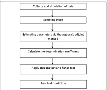
In this paper, a case study is presented on predicting patients with Alzheimer’s dis-ease risk. Unfortunately, none of the previously presented studies in literature provides sufficient data to perform our study. Therefore and instead of collecting data from lit-erature, a simulated dataset is generated. Other studies in literature were based on simu-lated datasets such as Tresch et al. [44], Giglio et al. [45], Murray et al. [46]. To define the predictors of the current study, we were based on previous studies highlighting the importance of physical exercises, feeding, quality of life and existence of a parent with Alzheimer disease. Based on those factors, the aim of the study is to give a percentage of Alzheimer’s disease risk for each individual in a population. Since, multiple predictors are involved and the outcome we aim to obtain is quantitative, multiple regression is the most suited statistical model to perform the study [16]. The theoretical bases of regres-sion are explained thereafter. The steps undertaken in this study are presented in Fig. 1.
The regression analysis is a statistical model that indicates how the variables are related on the basis of an equation. Formally, the variable we are trying to predict is
called dependent variable, the variable or variables to predict the value of the dependent variable are called independent variables (predictors). The simple regression is a regres-sion with single independent variable. The multiple regresregres-sion is a regresregres-sion with multi-ple independent variables. The procedures to accomplish simmulti-ple and multimulti-ple regression are in somehow similar.
The simple regression
Assuming the case where the Alzheimer’s disease risk is predicted on the base of one predictor, for instance, the age of a patient. The population undertaken in this study is a population of patients recorded in a dataset. The aim is to predict the percentage of Alz-heimer’s disease risk denoted y on the base of the patient age denoted x1.
The Eq. (1) describes the relation binding x and y with an error term denoted ɛ, cor-responds to a regression model. The model used in a simple regression is written as follows:
β0 and β1 correspond to the parameters of the population and ɛ is a random varia-ble called the error term. The error term takes into account the variability that is not explained by the linear relation between x and y.
The patient population can be seen as the set of subpopulations related to a given value of x. Thus, one of the subpopulations consists of all patients that already reached the 60s. Each sub-population has a particular distribution of y. Thus a distribution of y is associated with the patients that already reached the sixties. Each distribution of y values has its own mean or mathematical expectation. The equation which describes how the average or the mathematical expectation of y, denoted E(x), is related to x, is called the regression equation. The regression equation is written as follows:
β0 and β1 are unknown parameters. Subsequently, we will use the statistical procedure named the least squares estimation to estimate the values of β0 and β1 . Sample statistics
b0 and b1 are sample statistics used to estimate β0 and β1.
The multiple regression
Assuming the case where the Alzheimer’s disease risk is predicted on the base of several predictors, for instance, the age of a patient, the geographical area, the number of work hour, the physical exercises ‘hours, the existence of a parent with Alzheimer’s disease, the feeding, and the existence of Lyme disease risk. The population undertaken in this study is a population of patients recorded in a dataset. The aim is to predict the per-centage of Alzheimer’s disease risk denoted on the base of the predictors pinpointed out above.
The Eq. (3) that describes the relation binding xi and y with an error term denoted ɛ,
corresponds to a regression model. The model used in a multiple regression is written as follows:
(1)
y=β0+β1x+ε
(2)
E(x)=β0+β1x
(3)
The equation which describes how the average or the mathematical expectation of y, denoted E(x), is related to xi, is called the regression equation. The regression equation is
written as follows:
βi∈[0,k] are unknown parameters. Subsequently we will use the statistical procedure named the least squares estimation to estimate the values of βi∈[0,k] . The statistics bi∈[0,k] are sample statistics used to estimate βi∈[0,k].
The Alzheimer’s disease prediction statistical model
As we pointed out earlier in this paper, we believe that seven predictors have a great impact on predicting the Alzheimer’s disease risk. The first predictor denoted x1 is the age of an individual. The second predictor denoted x2 is the geographical area. The third one denoted x3 is the work’s hours per a day. The fourth one denoted x4 is the physical exercises’ hours. The fifth one denoted x5 is the existence of a parent with Alzheimer’s disease. The sixth one denoted x6 is the quality of feeding. The seventh and the last pre-dictors denoted x7 is the existence of Lyme disease. In conducting a statistical study, we would like to answer the following questions: do these variables really impact the Alz-heimer’s disease risk? Is there a relationship between the variables? If so, define this rela-tionship. Can the values of these parameters be adjusted in order to efficiently predict the Alzheimer’s disease risk?
Let assume that x1i is the random variable associating the age to an individual i. x2i is
the random variable associating a number indicating an area to an individual i. x3i is the
random variable associating a number indicating the work’s hours per a day to an indi-vidual i. x4i is the random variable associating a number indicating the work’s hours per
a day to an individual i. x5i is the random variable associating a number indicating the
existence or absence of a parent with Alzheimer disease for an individual i. x6i is the
ran-dom variable associating a number indicating the quality of feeding of an individual i. x7i
is the random variable associating a number indicating the existence of Lyme disease for an individual i. The regression model that describes the studies is as follows:
Throughout this paper, the steps undertaken to estimate the unknown parameters
βi∈[0,7] are explained in details. The next section explains the sampling stage. The Alzheimer’s disease prediction sampling stage
The sampling stage is a fundamental stage that has a great impact on the accuracy of the prediction model. Indeed, a small sample or a sample with similar individuals could lead to an inaccurate model [42]. Thus, sampling efficiently means predict efficiently. To tackle the problem of small samples a great number of statistical methods renowned for predicting efficiently based on small sample such as Hurvich and Tsai [47]. In addi-tion, the central limit theorem could be applied when the population is large. This theo-rem states that the sampling distribution of the sample mean can be approximated by a normal probability distribution in the case of large sample. In practice, the sampling
(4) E(x)=β0+β1x1+β2x2+ · · · +βkxk
(5)
distribution can be approximated by a normal distribution when the sample size is greater than or equal to 30 [42].
To proceed the sampling stage, the proposed solution randomly picks up an individ-ual. Then, compare it with the previously picked ones. If it is not similar or has close pro-prieties to any previously picked individual, it is added to the sample. The pseudo-code below details the steps token to accomplish the sampling stage.
The function notsimilar takes a patient as an income and returns a Boolean as an out-come. The function compares each attribute of the income to the attributes of the sam-ple if there is any similarity the function returns false. Otherwise it returns true.
The Adjoint method for the least squares estimation problem
To estimate the unknown parameters βi∈[0,k] Least Squares Estimation is the most com-mon method used [20]. The QR factorization solve the problem of ordinary least squares [20]. The reference [20] relates step by step Least Squares Estimation method. Briefly, estimating the unknown parameters βi∈[0,k] is equivalent to solve k equations system
with k unknowns. In our case and in contrast with the literature the Adjoint method is used to solve the k equations system. As a matter of fact, the system of equations can be expressed in a compact form by using matrix notation. The notation is as follows:
where n denotes the sample size and where: A·B=Y A=
n �ni=1x2i . . . �ni=1xki �n
i=1x2i �ni=1x22i . . . �n
i=1x2ixki .
.
. ... . .. ... �n
i=1xki �ni=1xkix2i . . . �ni=1x2ki ,B=
b0 b1 . . . bk ,Y =
�n i=1yi �n
i=1x2iyi . . . �n
This part of code was tested against large scale data to discover its limits. Unfortu-nately, this method suffers from shortcomings when the patients ‘sample is large and when the number of predictors is colossal. To overcome those shortcomings a new com-putational approach is presented thereafter. This method is massively parallel to absorb the massive calculations and to increase the method performance.
MR‑AM: MapReduce with Adjoint method
MapReduce is a programming model for data processing [48]. It enables distributed algorithms in parallel on clusters of machines with varied features. MApReduce also handles the parallel computation issues thus the users deploy their efforts on pro-gramming model. Since its advent MapReduce has gained popularity in both scientific community and firms due to its effectiveness in parallel processing [49]. Indeed, the par-allelization of QR factorization and SVD matrix decomposition methods is a relevant example of the scientific community interest toward MapReduce. The authors of Ben-son et al. [50] reported the matrix decomposition methods implemented on MapReduce programming. As pointed out earlier, the QR factorization is the most common method used to solve the least squares estimation problem. To the best of our knowledge, the Adjoint method has not been yet implemented on MapReduce framework. Thus, in this paper an implementation of Adjoint method on MapReduce is detailed in the aim to solve the least squares estimation problem.
Working within map reduce requires redesigning the traditional algorithms. As a mat-ter of fact, the computation is expressed as two phases: Map and reduce. Each phase has key-value pairs as input and output. Two functions should also be specified: the map function and the reduce function. The types of key-value pairs may be chosen by the programmer.
MapReduce breaks the processing into two phases: The map phase and the reduce phase. Each phase has (key, value) pairs as input and output. In the current study, a text input format represents each line in the dataset as a text value. The key is the first num-ber departed by a plus sign from the reminder of the line. Consider the following sample lines of input data:
The keys is the line numbers of the A matrix. The map function calculates the determi-nant for B matrix. The output of the Map function is as follows:
The pseudo code of Map Function is as follows:
The output from the map function is processed by the MapReduce framework before being sent to the reduce function. This processing sorts and groups the key-value pairs by key. So, continuing the example, our reduce function sees the following input:
0+067−011−95. . .
0+143−101−22. . .
1+243−011−22. . .
. .
. . .. . .. ...
. .
. . .. . .. ...
. .
. . .. . .. ...
4+340−310−12. . .
4+44−301−265. . .
(0, 1 0) (0, 22) (1, 11)
. . . . .. ...
The reduce function returns (i, βi) as output. The output of the reduce function is as
follows:
The pseudo code of Reduce Function is as follows:
Evaluation and experimental results
In this section, we evaluate the accuracy and the performance of the proposed model on simulated data based on actual data of Riskalz dataset and of previous studies. To validate the resulting model and to evaluate its strength, the proposed solution involves additional steps that are detailed thereafter.
Prediction accuracy measures
The reduction of error (RE) assumes a central role in the verification procedure [51]. RE is an example of a forecast skill statistic. The forecast skill is defined as the relative
(0,[10, 22]) (1,[11, 111])
. . . . .. ...
. . . . .. ...
. . . . .. ...
(4,[78, 80])
(0, 2) (1, 5) (2, 6.5)
accuracy of a set of forecasts which are usually the average values of the predictions. The equation used to calculate RE can be expressed in the following Eq. (6):
where SSEv the sum of squares of validation errors between is observed and predicted
values over the validation period and SSEref is the sum of squares of validation errors
between observed values and mean of the predictions often known as control values or reference values over the validation period. The difference between observed and predicted values is defined as validation error noted as e(i). It can be mathematically expressed as Eq. (7).
where Yi and Yˆ(i) are the observed and predicted values of the predictions for validation
data point i. The sum of the squares of errors for validation, SSEv, can be expressed as
Eq. (8) and the sum of squares of errors for reference, SSEref, can be expressed as Eq. (9).
where nv denotes the total number of data points in the validation dataset and Yˆ is the
mean of the prediction, which usually serves as a reference or control value. Theoreti-cally, the value of RE can range from negative infinity to one, where one indicates perfect prediction for the validation data set. It will only occur when all the residuals for valida-tion data are zero. On the other hand, if SSEv is much greater than SSEref, RE can be
neg-ative and large. A positive RE indicates that the regression model on average has some forecast skill. Contrastingly, if RE ≤ 0, the model is deemed to have no skill to predict. The similarity in form of the equations for RE and regression R2 expressed as Eq. (10) suggests that RE can also be used as validation evidence for R2. The closer the values of RE and R2 are to each other, the more the model is accepted as a predictive tool.
Fisher’s, Student’s test and correlation coefficient
Fisher’s F-test, also called global significance test; is used to determine if there is a sig-nificant relationship between the dependent variable and the set of independent vari-ables. However, Student’s t test, called individual significance test, is used to determine whether each of the independent variables is significant. A Student test is performed for each model-independent variable.
(6)
RE=1− SSEv SSEref
(7)
e(i)=Yi− ˆY(i)
(8)
SSEv =
nv
i=1
e2(i)
(9) SSEref =
nv
i=1
(Yi− ˆY(i))2
(10)
R2=1− SSE
SSE =1−
n
i=1(Yi−Yi)2
n
A correlation test is performed between the independent variables of the model. If the correlation coefficient between two variables is greater than 0.70, it is not possible to determine the effect of a particular independent variable on the dependent variable.
A Fisher’s test, based on Fisher’s distribution, can be used to test whether a relation-ship is meaningful. With a single independent variable, the Fisher’s test leads to the same conclusion as the Student test. On the other hand, with more than one independent var-iable, only the F test can be used to test the overall meaning of a relationship.
The logic underlying the use of the Fisher’s test to determine whether the relationship is statistically significant or not, is based on the construction of two independent esti-mates of σ2.
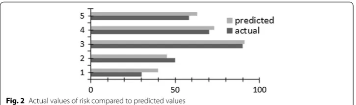
On the basis of the output model a punctual prediction is performed in this work. The Fig. 2 reports a comparison study carried out between the predicted value and the actual value of Alzheimer’s disease risk.
Experiments
In this section, we test the proposed method on three datasets to confirm its robustness. For each case study, a brief description is given. At the end of this section, we carried out experiments and we compared the actual and predicted values for each case study.
a. Student performance case study
The dataset was collected by using school reports and questionnaires. The collected data approaches students achievement in secondary education of two Portuguese schools. The data attributes include student grades, demographic, social and school related features.
Two datasets are provided regarding the performance in two distinct subjects: Math-ematics (mat) and Portuguese language (por).
In the current study, apply our approach to predict the G3 attributes on the basis of the reminder ones. An exhaustive list of attributes and their description could be found at http://archi ve.ics.uci.edu/ml/datas ets/Stude nt+Perfo rmanc e.
b. Parkinsons telemonitoring case study
The dataset is composed of a range of biomedical voice measurements from 42 people with early-stage Parkinson’s disease recruited to a 6-month trial of a telemonitoring device for remote symptom progression monitoring. The recordings were automatically captured in the patient’s homes.
The main aim of the data is to predict the motor and total UPDRS scores (‘motor_ UPDRS’ and ‘total_UPDRS’) from the 16 voice measures. For more details readers could refers to https ://archi ve.ics.uci.edu/ml/datas ets/Parki nsons +Telem onito ring.
c. The Levenson self report psychopathy scale value case study
The data used to construct the prediction model is similar to the one used to spot sexual offenders available at http://resha re.ukdat aserv ice.ac.uk/85252 1. Based on the factors provided in the studies of Ian Mitchell we aim to predict the value of the first and the second factors of LSRP measure. The following variable codes are relevant to aaFHNeye-sAccuracyData, aaFHNeyesDwellTime and aaFHNeyesFix Count datasets:
• Participant = Identification number assigned to participant
• Eye tracker = Method of eye tracking (1 = head mounted; 2 = tower)
• Primary = Primary subscale of the Levenson Self Report Psychopathy Scale
• Secondary = Secondary subscale of the Levenson Self Report Psychopathy Scale
Variable names for each trial type are coded as follows [Emotion] [Intensity] [Sex] [Region] using the following values:
• Emotion: ANG = Angry expression, DIS = Disgust expression, FEAR = Fear expres-sion, HAP = Happy expression, SAD = Sad expression, SUR = Surprise expression
• Intensity: 5 = 55, 9 = 90
• Sex: F = Female, M = male
• Region: Eyes = Eyes, Mouth = Mouth
Thus, ANG 5 F refers to an angry expression at 55% intensity, expressed by a female face and ANG 5 F Eyes refers to the eye region of the same face.
d. The comparative study
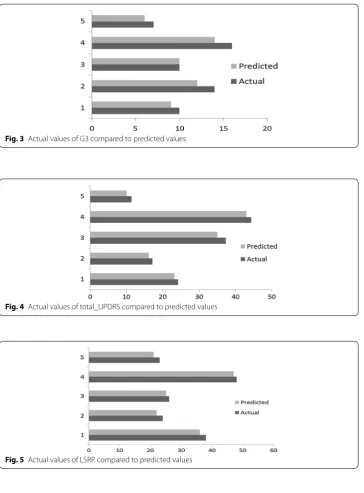
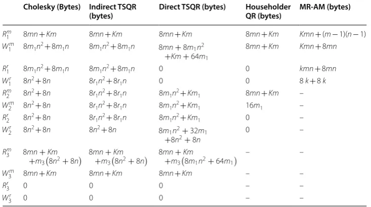
On the basis of the output model a punctual prediction is performed for each case study described above. The Figs. 3, 4, 5 report a comparison study carried out between the predicted value and the actual value of the predicted attribute.
Discussion
In this section we conducted a comparative study with the aim to position the proposed method within the methods solving the least square problem. Therefore, we use the Hadoop job performance model to estimate the job completion time given by Khan et al. [52].
In the current paper, we estimate the lower bound for a job with N iterations. For this purpose, Hadoop benchmarks are used to estimate the inverse of read and write bandwidth respectively denoted βr and βw . In addition, the limit number of maps and reduces, respectively denoted mmax and rmax, should be fixed in the Hadoop
configura-tion. The Lower bound for a job with N iterations, denoted Tlb, is estimated on the basis
Subject to:
(11)
Tlb= N
j=1
Rwj βr+wmj βw
pjm +
Rjrβr+wjrβw
prj
(12)
pmj =minmmax,mj
(13) prj =minrmax,rj,kj
Fig. 3 Actual values of G3 compared to predicted values
Fig. 4 Actual values of total_UPDRS compared to predicted values
where kj is the number of distinct input keys passed to the reduce tasks for step j and
where mj and rj are respectively the number of map and reduce tasks for step j.
In the current subsection, we analyze the efficiency of the proposed MapReduce-based Adjoint method by comparing it with state-of-the-art of the parallelized factorization method such as:
1. Cholesky Benson et al. [50], 2. Indirect TSQR Benson et al. [50], 3. Direct TSQR Benson et al. [50], 4. Householder QR Benson et al. [50].
(14) Rmj =number of data read in the jth map
(15)
Rrj =number of data read in the jth reduce
(16)
wmj =number of data write in the jth map
(17)
wrj =number of data write in the jth reduce
Table 1 The estimated βr and βw values for different HDFS file sizes HDFS Size (GB) Write (MB/s) Read (MB/s) βw
(s/MB) β(s/MB)r
1 67.72 60.25 0.015 0.017
32 61.39 85.91 0.016 0.012
64 81.22 83.91 0.012 0.012
128 79.56 76.15 0.013 0.013
Table 2 Number of reads and writes at each step (in bytes)
We assume a double is 8 bytes and is the number of bytes for a key. The amount of key data is separated from the amount of value data
Cholesky (Bytes) Indirect TSQR
(bytes) Direct TSQR (bytes) Householder QR (bytes) MR‑AM (bytes)
Rm
1 8mn+Km 8mn+Km 8mn+Km 8mn+Km Kmn+ (m− 1)(n− 1) W1m 8m1n2+ 8m1n 8m1n2+ 8m1n 8mn+8m1n2
+Km+64m1
8mn+Km Kmn+ 8mn
Rr1 8m1n2+ 8m1n 8m1n2+ 8m1n 0 0 kmn+ 8mn W1r 8n2+ 8n 8r1n2+ 8r1n 0 0 8 k+ 8 k Rm
2 8n2+ 8n 8r1n2+ 8r1n 8m1n2+Km1 8mn+Km –
Wm
2 8n2+ 8n 8r1n2+ 8r1n 8m1n2+Km1 16m1 –
Rr
2 8n2+ 8n 8r1n2+ 8r1n 8m1n2+Km1 0 –
Wr
2 8n2+ 8n 8n2+ 8n 8m1n2+32m1
+8n2
+8n
0 –
Rm3 8mn+Km
+m38n2+8n
8mn+Km
+m38n2+8n
8mn+Km
+m38m1n2+64m1
– –
Wm
3 8mn+Km 8mn+Km 8mn+Km – –
Rr
3 0 0 0 – –
This set of algorithms represents is the set of parallel method based on MapReduce to solve the least square problem.
We conduct several groups of experiments on a local machine equipped with only 2 cores. To estimate βr and βw , we used Hadoop benchmarks. Tables 1, 2 provides βr and
βw values for different HDFS file sizes. Table 2 provides the number of reads and writes for state-of-the-art of the parallelized factorization methods and our proposed parallel-ized Adjoint algorithm. The computed lower bounds are contained in Table 3.
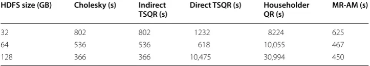
The Tables 2 and 3 confirms the performance of the proposed solution is competitive with existing methods in terms of number of operations and computational time.
Conclusion
In this paper, we carry out a comparative study between the parallel methods aiming to solve the least square estimation problem and our proposal. The results promote the use of the proposed method as the results confirm its efficiency and rapidity. Moreover, we presents a detailed description of the parallel MapReduce-based Adjoint method. The application of the method to predict the Alzheimer’s disease risk confirms its robustness. Authors’ contributions
Authors propose a solution which receives a dataset of patients with a variable number of attributes and then constructs a statistical model to spot eventual Alzheimer’s disease patients. Authors parallelize the Adjoint method via MapReduce to this aim. All authors read and approved the final manuscript.
Acknowledgements
Not applicable.
Competing interests
The authors declare that they have no competing interests.
Availability of data and materials
Not applicable.
Consent for publication
Not applicable.
Ethics approval and consent to participate
Not applicable.
Funding
Not applicable.
Publisher’s Note
Springer Nature remains neutral with regard to jurisdictional claims in published maps and institutional affiliations.
Received: 4 May 2018 Accepted: 25 July 2018
Table 3 The computed lower bounds Tlb in seconds HDFS size (GB) Cholesky (s) Indirect
TSQR (s) Direct TSQR (s) Householder QR (s) MR‑AM (s)
32 802 802 1232 8224 625
64 536 536 618 10,055 467
References
1. Li L, Ge RL, Zhou SM, Valerdi R. Guest editorial integrated healthcare information systems. IEEE Trans Inf Technol Biomed. 2012;16(4):515–7. https ://doi.org/10.1109/TITB.2012.21983 17.
2. Kumar A, Hancke GP. A Zigbee-based animal health monitoring system. IEEE Sens J. 2015;15(1):610–7. https ://doi. org/10.1109/JSEN.2014.23490 73.
3. Luke DA, Stamatakis KA. Systems science methods in public health: dynamics, networks, and agents. Annu Rev Public Health. 2012;33(1):357–76. https ://doi.org/10.1146/annur ev-publh ealth -03121 0-10122 2.
4. Ferreira LK, Busatto GF. Neuroimaging in Alzheimer’s disease: current role in clinical practice and potential future applications. Clinics. 2011;66(Suppl 1):19–24. https ://doi.org/10.1590/S1807 -59322 01100 13000 03.
5. Soucy JP, Bartha R, Bocti C, Borrie M, Burhan AM, Laforce R, Rosa-Neto P. Clinical applications of neuroimaging in patients with Alzheimer’s disease: a review from the Fourth Canadian consensus conference on the diagnosis and treatment of Dementia 2012. Alzheimer’s Res Ther. 2013;5(1):S3. https ://doi.org/10.1186/alzrt 199.
6. Thambisetty M, Lovestone S. Blood-based biomarkers of Alzheimer’s disease: challenging but feasible. Biomarkers Med. 2010;4(1):65–79.
7. Lutz MW, Sundseth SS, Burns DK, Saunders AM, Hayden KM, Burke JR, Roses AD. A genetics-based biomarker risk algorithm for predicting risk of Alzheimer’s disease. Alzheimer’s Dementia Transl Res Clin Intervent. 2016;2(1):30–44.
https ://doi.org/10.1016/j.trci.2015.12.002.
8. Liu-Ambrose T, Eng JJ, Boyd LA, Jacova C, Davis JC, Bryan S, Hsiung G-YR. Promotion of the mind through exercise (PROMoTE): a proof-of-concept randomized controlled trial of aerobic exercise training in older adults with vascular cognitive impairment. BMC Neurol. 2010;10(1):14. https ://doi.org/10.1186/1471-2377-10-14.
9. Scarmeas N, Luchsinger JA, Schupf N, et al. Physical activity, diet, and risk of Alzheimer disease. JAMA. 2009;302(6):627–37. https ://doi.org/10.1001/jama.2009.1144.
10. Nemati Karimooy H, Hosseini M, Nemati M, Esmaily HO. Lifelong physical activity affects mini mental state exam scores in individuals over 55 years of age. J Bodyw Mov Ther. 2012;16(2):230–5. https ://doi.org/10.1016/j. jbmt.2011.08.003.
11. Winchester J, Dick MB, Gillen D, Reed B, Miller B, Tinklenberg J, Cotman CW. Walking stabilizes cognitive functioning in Alzheimer’s disease (AD) across 1 year. Arch Gerontol Geriatr. 2013;56(1):96–103. https ://doi.org/10.1016/j.archg er.2012.06.016.
12. Bu X-L, Yao X-Q, Jiao S-S, Zeng F, Liu Y-H, Xiang Y, Wang Y-J. A study on the association between infectious burden and Alzheimer’s disease. Eur J Neurol. 2015;22(12):1519–25. https ://doi.org/10.1111/ene.12477 .
13. Maheshwari P, Eslick GD. Bacterial infection and Alzheimer’s disease: a meta-analysis. J Alzheimer’s Dis. 2015;43(3):957–66. https ://doi.org/10.3233/JAD-14062 1.
14. MacDonald AB. Plaques of Alzheimer’s disease originate from cysts of Borrelia burgdorferi, the Lyme disease spiro-chete. Med Hypotheses. 2006;67(3):592–600. https ://doi.org/10.1016/j.mehy.2006.02.035.
15. Zettam M, Laassiri J, Enneya N. A software solution for preventing Alzheimer’s disease based on MapReduce framework. In: 2017 IEEE international conference on information reuse and integration (IRI). San Diego, CA; 2017. p. 192–7. https ://doi.org/10.1109/iri.2017.77.
16. Hastie T, Tibshirani R, Friedman J. The elements of statistical learning data mining, inference, and prediction. New York: Springer; 2009. https ://doi.org/10.1007/978-0-387-84858 -7_1.
17. Michie D, Spiegelhalter DJ, Taylor CC, Campbell J, editors. Machine learning, neural and statistical classification. Upper Saddle River: Ellis Horwood; 1994.
18. Tu JV. Advantages and disadvantages of using artificial neural networks versus logistic regression for predicting medical outcomes. J Clin Epidemiol. 1996;49(11):1225–31. https ://doi.org/10.1016/S0895 -4356(96)00002 -9. 19. Hosmer DW, Lemeshow S. Applied logistic regression. 2nd ed. Hoboken: John Wiley & Sons Inc.; 2005. https ://doi.
org/10.1002/04717 22146 .fmatt er.
20. Rencher AC, Christensen WF. Methods of multivariate analysis. 3rd ed. Hoboken: Wiley; 2012.
21. Steyerberg EW. Clinical prediction models: a practical approach to development, validation, and updating. New York: Springer; 2008.
22. Lecleire S, Di Fiore F, Antonietti M, Ben Soussan E, Hellot M-F, Grigioni S, P Ducrotté. Undernutrition is predictive of early mortality after palliative self-expanding metal stent insertion in patients with inoperable or recurrent esopha-geal cancer. Gastrointest Endosc. 2006;64(4):479–84. https ://doi.org/10.1016/j.gie.2006.03.930.
23. Janssen-Heijnen MLG, Houterman S, Lemmens V, Brenner H, Steyerberg EW, Coebergh JWW. Prognosis for long-term survivors of cancer. Ann Oncol. 2007;18(8):1408–13. https ://doi.org/10.1093/annon c/mdm12 7.
24. Chatap NJ, Shrivastava AK. A survey on various classification techniques for medical image data. Int J Comput Appl. 2014;97(15):1–5.
25. Breiman L, Friedman J, Stone CJ, Olshen RA. Classification and regression trees. New ed. Boca Raton: Taylor & Francis Ltd.; 1984.
26. Quinlan JR. Comparing connectionist and symbolic learning methods. In: Hanson SJ, Rivest RL, Drastal GA, editors. Proceedings of a workshop on computational learning theory and natural learning systems: constraints and pros-pects, vol. 1. Cambridge: MIT Press; 1994. p. 445–56.
27. Kass GV. An exploratory technique for investigating large quantities of categorical data. J Roy Stat Soc Ser C (Appl Stat). 1980;29(2):119–27.
28. Lim T-S, Loh W-Y, Shih Y-S. A comparison of prediction accuracy, complexity, and training time of thirty-three old and new classification algorithms. Mach Learn. 2000;40(3):203–28. https ://doi.org/10.1023/A:10076 08224 229. 29. Klecka WR. Discriminant analysis. 1st ed. Beverly Hills: SAGE Publications Inc.; 1980.
30. Hinton GE. How neural networks learn from experience. Sci Am. 1992;267(3):144–51.
31. Rumelhart DE, Hinton GE, Williams RJ. Learning representations by back-propagating errors. Nature. 1986;323(6088):533–6. https ://doi.org/10.1038/32353 3a0.
32. Szolovits P, Patil RS, Schwartz WB. ARtificial intelligence in medical diagnosis. Ann Intern Med. 1988;108(1):80–7.
33. Spelt L, Andersson B, Nilsson J, Andersson R. Prognostic models for outcome following liver resection for colorectal cancer metastases: a systematic review. Eur J Surg Oncol. 2012;38(1):16–24. https ://doi.org/10.1016/j. ejso.2011.10.013.
34. Mortazavi D, Kouzani AZ, Soltanian-Zadeh H. Segmentation of multiple sclerosis lesions in MR images: a review. Neuroradiology. 2012;54(4):299–320. https ://doi.org/10.1007/s0023 4-011-0886-7.
35. Ahmed FE. Artificial neural networks for diagnosis and survival prediction in colon cancer. Mol Cancer. 2005;4(1):29.
https ://doi.org/10.1186/1476-4598-4-29.
36. Bartosch-Härlid A, Andersson B, Aho U, Nilsson J, Andersson R. Artificial neural networks in pancreatic disease. Br J Surg. 2008;95(7):817–26. https ://doi.org/10.1002/bjs.6239.
37. Siristatidis CS, Chrelias C, Pouliakis A, Katsimanis E, Kassanos D. Artificial neural networks in gynaecological diseases: current and potential future applications. Med Sci Monit Int Med J Exp Clin Res. 2010;16(10):RA231–6.
38. Shankaracharya DO, Samanta S, Vidyarthi AS. Computational intelligence in early diabetes diagnosis: a review. Rev Diabet Stud RDS. 2010;7(4):252–62. https ://doi.org/10.1900/RDS.2010.7.252.
39. Amato F, López A, Peña-Méndez EM, Vaňhara P, Hampl A, Havel J. Artificial neural networks in medical diagnosis. J Appl Biomed. 2013;11(2):47–58. https ://doi.org/10.2478/v1013 6-012-0031-x.
40. Cesa-Bianchi N, Lugosi G. Prediction, learning, and games. Cambridge: Cambridge University Press; 2006. 41. Chen Y, Crespi N, Ortiz AM, Shu L. Reality mining: a prediction algorithm for disease dynamics based on mobile big
data. Inf Sci. 2017;379:82–93. https ://doi.org/10.1016/j.ins.2016.07.075.
42. Anderson DR, Sweeney DJ, Williams TA, Camm JD, Cochran JJ. Statistiques pour l’économie et la gestion, 5e édition. De Boeck Universite; 2015.
43. Tribout B. Statistiques pour économistes et gestionnaires. London: Pearson Education; 2008.
44. Tresch MC, Cheung VCK, d’Avella A. Matrix factorization algorithms for the identification of muscle synergies: evaluation on simulated and experimental data sets. J Neurophysiol. 2006;95(4):2199–212. https ://doi.org/10.1152/ jn.00222 .2005.
45. Giglio L, Kendall JD, Justice CO. Evaluation of global fire detection algorithms using simulated AVHRR infrared data. Int J Remote Sens. 1999;20(10):1947–85. https ://doi.org/10.1080/01431 16992 12290 .
46. Murray RE, Ryan PB, Reisinger SJ. Design and validation of a data simulation model for longitudinal healthcare data. AMIA Ann Symp Proc. 2011;2011:1176–85.
47. Hurvich CM, Tsai C-L. Regression and time series model selection in small samples. Biometrika. 1989;76(2):297–307.
https ://doi.org/10.2307/23366 63.
48. White T. Hadoop: the definitive guide. Farnham: O’Reilly Media Inc; 2009.
49. Dean J, Ghemawat S. MapReduce: simplified data processing on large clusters. Commun ACM. 2008;51(1):107–13.
https ://doi.org/10.1145/13274 52.13274 92.
50. Benson AR, Gleich DF, Demmel J. Direct QR factorizations for tall-and-skinny matrices in MapReduce architectures. In: 2013 IEEE international conference on big data; 2013. p. 264–72. https ://doi.org/10.1109/BigDa ta.2013.66915 83. 51. Lu P, Pei S, Tolliver D. Regression model evaluation for highway bridge component deterioration using national
bridge inventory data. J Transp Res Forum. 2016;55(1):5–16.