R E G U L A R A R T I C L E
Open Access
Centrality in modular networks
Zakariya Ghalmane
1,3, Mohammed El Hassouni
1, Chantal Cherifi
2and Hocine Cherifi
3**Correspondence:
hocine.cherifi@u-bourgogne.fr
3LE2I, UMR6306 CNRS, University of
Burgundy, Dijon, France Full list of author information is available at the end of the article
Abstract
Identifying influential nodes in a network is a fundamental issue due to its wide applications, such as accelerating information diffusion or halting virus spreading. Many measures based on the network topology have emerged over the years to identify influential nodes such as Betweenness, Closeness, and Eigenvalue centrality. However, although most real-world networks are made of groups of tightly
connected nodes which are sparsely connected with the rest of the network in a so-called modular structure, few measures exploit this property. Recent works have shown that it has a significant effect on the dynamics of networks. In a modular network, a node has two types of influence: a local influence (on the nodes of its community) through its intra-community links and a global influence (on the nodes in other communities) through its inter-community links. Depending on the strength of the community structure, these two components are more or less influential. Based on this idea, we propose to extend all the standard centrality measures defined for networks with no community structure to modular networks. The so-called “Modular centrality” is a two-dimensional vector. Its first component quantifies the local influence of a node in its community while the second component quantifies its global influence on the other communities of the network. In order to illustrate the effectiveness of the Modular centrality extensions, comparison with their scalar counterparts is performed in an epidemic process setting. Simulation results using the Susceptible-Infected-Recovered (SIR) model on synthetic networks with controlled community structure allows getting a clear idea about the relation between the strength of the community structure and the major type of influence (global/local). Furthermore, experiments on real-world networks demonstrate the merit of this approach.
Keywords: Influential nodes; Centrality measures; Community Structure; SIR model
1 Introduction
Identifying the most influential nodes in a network has gained much attention among re-searchers in recent years due to its many applications. Indeed, these key nodes play a major role in controlling the epidemic outbreak [1], increasing the publicity on a new product [2], controlling the rumor spreading [3]. The most popular approach to uncover these central nodes is to quantify their influence using centrality measures. Various centrality measures have been proposed to quantify the influence of nodes based on their topological prop-erties. Degree centrality, betweenness centrality, closeness centrality are among the most basic and the most widely used centrality measures.
The majority of real-world networks exhibit the modular organization of nodes, the so-called community structure [4–8]. Although there has been a tremendous effort regarding
the definition of this property, there is no formal consensus on a definition that captures the gist of a community. It is intuitively apprehended as densely connected groups of nodes where individuals interact with each other more intensely than with those in the rest of the network. Therefore, communities are groups of nodes sharing some common proper-ties and play similar roles in the interacting phenomenon within networks. Besides their various definitions, communities have been also found to show a number of interesting features such as the overlapping configuration of modules [9]. Some of the nodes can then be shared by multiple communities. Indeed, in some social networks, individuals can take part simultaneously in different groups, such as work colleagues, friends or family. In this work, we do not consider the overlaps between communities.
Previous works have shown that community structure has an important effect on the spreading process in networks [10–13]. However, classical centrality measures [14] do not take into account the influence of this major topological property on the spreading dynamics. In a modular network, we can distinguish two types of links [15,16] that sup-port the diffusion process: the links that connect nodes belonging to the same community (intra-community links or strong ties) and the links that bridge the communities (inter-community links or weak ties). The former exercise a local influence on the diffusion pro-cess (i.e., at the community level), while the latter have a global influence (at the network level). Therefore, we believe that these two types of links should be treated differently. In-deed, the intra-community links contribute to the diffusion in localized densely connected areas of the networks, while the inter-community links allow the propagation to remote areas of the network. Suppose that an epidemic starts in a community, as it is highly con-nected, the intra-community links will tend to confine the epidemic inside the commu-nity, while the inter-community links will tend to propagate it to the other communities. As their role is quite different, we propose to represent the centrality of modular networks by a two-dimensional vector where the first component quantifies the intra-community (or local) influence and the second component quantifies the inter-community (or global) influence of each individual node in the network. To compute these components, we need to split the original network into a local and global network. The local network is obtained by removing all the inter-community links from the original network. The global network is obtained by removing all the intra-community links from the original network. Note that if the original network is made of a single connected component the global and lo-cal networks split into many connected components. Therefore, care must be taken to adapt the centrality definition to networks with multiple components. In the following, we restrict our attention to non-overlapping community structure (i.e. a node belongs to a single community). Furthermore, we consider undirected and unweighted networks for the sake of simplicity, but results can be easily extended to more general situations.
The proposed approach can be summarized as follows: • Choose a standard centrality measure.
• Compute the local network by removing all the inter-community links from the modular network.
• Compute the Local component of the Modular centrality using the standard centrality. • Compute the global network by removing all the intra-community links from the
modular network.
As nodes need to be ranked according to their centrality values, it is necessary to adopt a strategy based on a combination of the two components of the Modular centrality. Various strategies, that include different levels of information about the community structure, may be used. As our main concern, in this paper, is to highlight the multidimensional nature of centrality in modular networks rather than devising optimal ranking methods, elementary strategies are evaluated. Two straightforward combination strategies (the modulus and the tangent of the argument of the Modular centrality) and a weighted linear combination of the components of the Modular centrality are investigated.
Experiments are conducted on modular synthetic networks in order to better under-stand the relative influence of the Local and Global component of the Modular central-ity in the propagation process. Extensive comparisons with the standard centralcentral-ity mea-sures show that Modular centrality meamea-sures provide more accurate rankings. Simulations on real-world networks of diverse nature have also been performed. As their community structure is unknown, a community detection algorithm has been used. Results confirm that node rankings based on the Modular centrality are more accurate in terms of the epi-demic size than those made by the standard centrality measures which have been designed for networks with no community structure.
The rest of the paper is organized as follows. Related modular-based measures are dis-cussed in the next section. In Sect.3, a general definition of the Modular centrality is given. In this framework, we present the extensions to modular networks of the most influential centrality measures (closeness, betweenness and eigenvector centrality). The experimen-tal setting is described in Sect.4. We report and analyze the results of the experiments performed on both synthetic and real-world networks in Sect.5. Finally, the main conclu-sions are presented in Sect.6.
2 Related works
Ranking the nodes according to their centrality constitutes the standard deterministic ap-proach to uncover the most influential nodes in a network. These measures rely usually on various network topological properties. However, the community structure of the network is rarely taken into consideration. Few researchers have paid attention to this property en-countered in many real-world networks [10–13,17–23]. In this section, we give a brief overview of the main deterministic methods that motivates our proposition.
a. Community centrality Newman proposed a slightly different formulation of the mod-uloarity. The Community centrality [24] is derived from the eigenvectors of the modularity matrix. Where the modularity matrix is divided into two projections. The first dimension represents the positive eigenvectors of the modularity matrix while the second dimension represents the negative ones. Thus, the modularity can be written in terms of these vectors as follows:
Q=
c
k=1
|Xk|2– c
k=1
|Yk|2, (1)
wherecis the number of communities.XandYare the community eigenvectors in both dimensions. Theith node in the communitykis represented by two vectorsxiandyi(the
The magnitude of a node vector|xi|specifies how central the nodeiis in its community
in terms of the number of connections. Thus, the nodeihas a large positive contribution to the modularity when this measure is large. On the other hand, a higher value of|yi|
means that the nodeihas many connections to other nodes from foreign communities. Therefore, the Community centrality is defined to be equal to the vector magnitude|xi|. It
measures the strength with which a given nodeiis assigned to its community. This mea-sure was tested in the network of co-authorships between scientists. Results show that it is not very correlated with the degree centrality. Moreover, some nodes with high Commu-nity centrality measure have a relatively low degree. However, they have more connections with nodes of their communities. Thus, nodes with high Community centrality value play a central role in the spreading process in their local neighborhood.
b. Comm centrality N. Gupta et al. [25] proposed a degree-based centrality measure for networks with non-overlapping community structure. It is based on a non-linear combi-nation of the number of intra-community links and inter-community links. The goal is to select nodes that are both hubs in their community and bridges between the commu-nities. This measure gives more importance to community bridges. Indeed, the number of inter-community links is raised to the power of two. The comparison has been per-formed with deterministic and random immunization strategies using the SIR epidemic model and both synthetic and real-world networks. Nodes are immunized sequentially from each community in the decreasing order of their centrality value in their respective community. The number of nodes to be removed from a community are kept proportional to the community size. Results show that the Comm strategy is more effective or at least works as well as Degree and Betweenness centrality while using only information at the community level.
c. Number of neighboring communities centrality In a previous work [26], we proposed to rank the nodes according to the number of neighboring communities that they reach in one hop. The reason for selecting these nodes is that they are more likely to have a big influence on nodes belonging to various communities. Simulation results on different synthetic and real-world networks show that it outperforms Degree, Betweenness and Comm centrality in term of the epidemic size in networks with a community structure of medium strength (i.e. when the average number of intra-community links is of the same order than the number of inter-community links).
A variation of this centrality measure called the Weighted Community Hub-Bridge cen-trality has also been introduced. It is weighted such that, in networks with well-defined community structure, more importance is given to bridges (inter-community links), while in networks with weak community structure the hubs in the communities dominate. The goal is to target the bridges or the hubs according to the community structure strength. This measure has proved its efficiency as compared to the alternatives particularly in net-works with weak community structure.
e. K-shell with community centrality Luo et al. proposed a variation of the K-shell de-composition for modular networks [27]. They suggest that the intra-community and the inter-community links should be considered separately in the K-core decomposition pro-cess. Their method works as follows:
(i) After the removal of nodes with intra-community links, the K-shell decomposition of the remaining nodes is computed. It is associated with an index ofkW
core.
(ii) After the removal of nodes with inter-community links, the K-shell of the remaining nodes is computed. It is associated with an index ofkS
core.
(iii) A new measure is then calculated and assigned to each node based on the linear combination of bothkW
coreandkcoreS in order to find nodes that are at the same time
bridges and hubs located in the core of the network.
Experiments have been performed using SIR simulations on Facebook friendship net-works at US Universities. Results show that this strategy is more efficient in term of the epidemic size than the classical K-shell decomposition, the Degree and the Betweenness centrality measures.
f. Global centrality In [28], M. Kitromilidis et al. propose to redefine the standard cen-trality measures in order to characterize the influence of Western artist. Based on the idea that influential artists have connections beyond their artistic movement, they propose to define the centrality of modular networks by considering only the inter-community links. In other words, an influential artist must be related to multiple communities, rather than being strongly embedded in its own community. Considering a painter collaboration network where edges between nodes represent biographical connections between artists, they compared Betweenness and Closeness centrality measures with their classical ver-sion. Results show that the correlation values between the standard and modified central-ity measures are quite high. However, the modified centralcentral-ity measures allow to highlight influential nodes who might have been missed as they do not necessarily rank high in the standard measures.
3 Modular centrality
Our main objective is to take into account the community structure in order to identify influential nodes. Indeed, in modular networks, a node has two types of influence: a local influence which is linked to its community features and a global influence related to its in-teractions with the other communities. Under this assumption, we provide a general defi-nition of centrality in modular networks. We design a generic algorithm for computing the centrality of a node under this general definition. The Modular centrality extension can be naturally inferred from the various existing definitions of centrality designed for networks without community structure. To illustrate this process, we give the modular extensions of the most influential centrality measures (Betweenness, Closeness, and Eigenvector).
3.1 Definitions
3.1.1 Local component of the Modular centrality
Let’s consider a network denoted asG(V,E), whereV={v1,v2, . . . ,vn}andE={(vi,vj)\
vi,vj∈V}denotes respectively the set of vertices and edges. Its non-overlapping
commu-nity structureCis a partition into a set of communitiesC={C1, . . . ,Ck, . . . ,Cm}whereCkis
thekth community andmis the number of communities. The local networkGlis formed
by the union of all the disjoint modules of the networkGl=
m
k=1Ck. These components
are obtained by removing all the inter-community links between modules from the orig-inal networkG. Each module represents a communityCk denoted asCk(Vk,Ek). Where
Vk={vki \vi∈V}andEk={(vki1,v k2
j )\vi,vj∈Vandk1=k2}, whilevki refers to any nodevi
belonging to the communityCk.
For a selected centrality measureβ, we defineβL(vki) as the Local centrality of the node
vi∈Vk. It is computed separately in each moduleCkof the local graphGl.
3.1.2 Global component of the Modular centrality
Let’s consider the network G(V,E), the global network Gg is formed by the union
of all the connected components of the graph that are obtained after removing all the intra-community links from the original network G(V,E). Let’s suppose that S =
{S1, . . . ,Sq, . . . ,Sp}is the set of the revealed connected components andp=|C|is the size
of the setS, the global network is defined byGg=
p
q=1Sq. Each componentSqis denoted
asSq(Vq,Eq). WhereVq={vqi\vi∈V}andEq={(vqi1,v q2
j )\vi,vj∈Vandq1=q2}, whilevqi
refers to any nodevibelonging to the componentSq. In this network, there may be some
isolated nodes (i.e., nodes that are not linked directly to another community). These nodes are removed fromGgin order to obtain a trimmed network formed only by nodes linked
to different communities by one hop. Consequently, the set of nodes ofGgis defined then
byVg={vi∈V\ |Nv1i| = 0}. WhereN
n
vi is the neighborhood set of nodes reachable inn hops. It is defined byNn
vi={vj∈V\vi=vjanddG(vi,vj)≤n},dGis the geodesic distance. For a selected centrality measureβ, we defineβG(vqi) as the Global centrality of the node
vi∈Vq. It is computed over each connected componentSqincluded in the global graph
Gg. Remember that the Global centrality measure of the removed isolated nodes is set to 0.
3.1.3 Modular centrality
It is a vector with two components. The first component quantifies the local influence of the nodes in their own community through the local graphGl, while the second
connected components of the global graphGg. The Modular centrality of a nodeviis given
by:
BM(vi) =
βL
vki,βG
vqi k∈ {1, . . . ,m}andq∈ {1, . . . ,p}, (2)
whereβLandβGrepresent respectively the Local and Global centrality of the nodevi.
3.2 Algorithm
The Modular centrality is computed as follows: Step 1. Choose a standard centrality measureβ.
Step 2. Remove all the inter-community links from the original networkGto obtain the set of communitiesCforming the local networkGl.
Step 3. Compute the Local measureβLfor each node in its own community.
Step 4. Remove all the intra-community links from the original network to reveal the set of connected componentsSformed by the inter-community links. Step 5. Form the global networkGgbased on the union of all the connected
component. Isolated nodes are removed from this network and their Global centrality value is set to 0.
Step 6. Compute the Global measureβGof the nodes linking the communities based on
each component of the global network.
Step 7. AddβLandβGto the Modular centrality vectorBM.
The pseudo-code of the algorithm to compute the Modular centrality is given in Algo-rithm1.
3.3 Modular extensions of standard centrality measures
In order to illustrate the process allowing to extend a given centrality defined for a network without community structure to a modular network, we give as examples the modular definitions of the Betweenness, Closeness and Eigenvector centrality.
3.3.1 Modular Betweeness centrality
The modular Betweeness centrality takes into account separately paths that start and finish in the same community and those which starts and finish in different communities. For a given nodevi, it is represented by the following vector:
BM(vi) =
βL
vki,βG
vqi k∈ {1, . . . ,m}andq∈ {1, . . . ,p}, (3)
where:
βL
vki=
vs,vt∈Ck
σstl(vi)
σstl , (4)
βG
vqi=
vs,vt∈Sq
σstg(vi)
σstg (5)
βLmeasures the Betweenness centrality of nodes in their own community andβG
Algorithm 1:Generic computation of the Modular centrality Input : GraphG(V,E), Centrality measureβ
Output: A mapM(node:centrality vector)
1 Remove all the inter-community links fromGto form the local networkGl
2 Remove all the intra-community links fromGto form the global networkGg
3 Create and initialize an empty mapM(node:BM)
4 BM(vi) = (βL(vik),βG(vqi)) represent the centrality vector, where each nodeviof the
network should be associated with its Local and Global value according to the selected centrality measureβ
5 foreach Ck⊂Gl, where k∈ {1, . . . ,m}do
6 foreach vk
i ∈Vkdo
7 CalculateβL(vki)
8 BM(vi).add(βL(vki))
9 end
10 end
11 foreach Sq⊂Gg, where q∈ {1, . . . ,p}do
12 foreach vqi ∈Vqdo
13 CalculateβG(vqi)
14 BM(vi).add(βG(vqi))
15 end
16 end
17 foreach vi∈Vdo
18 M.add(vi,BM(vi))
19 end
20 Return the mapM
network respectively, whileσstl(vi) andσstg(vi) represent the number of shortest paths
con-necting nodesvsandvtand passing throughviin the local and the global network
respec-tively.
3.3.2 Modular Closeness centrality
Modular Closeness centrality considers separately the shortest distances of nodes origi-nating from the same or from another community than the starting nodevi. It is defined
as follows:
BM(vi) =
βL
vki,βG
vqi k∈ {1, . . . ,m}andq∈ {1, . . . ,p}, (6)
where:
βL
vki= 1
vj∈Ckd
l ij
βG
vqi= 1
vj∈Sqd
g ij
(8)
βLandβGmeasure respectively the Local and Global component of the Modular
Close-ness centrality.dlijanddgijindicate the length of the geodesic from nodevito nodevjbased
on the local and the global network respectively.
3.3.3 Modular Eigenvector centrality
Modular Eigenvector takes into account separately both the number and the importance of the neighbors belonging to the same community and those belonging to different com-munities to measure its centrality. The community based Eigenvector of a nodeviis
de-fined by the following vector:
BM(vi) =
βL
vki,βG
vqi k∈ {1, . . . ,m}andq∈ {1, . . . ,p}, (9)
where:
βL
vki=1
λ
vj∈Ck aijβL
vkj, (10)
βG
vqi=1
λ
vj∈Sq aijβL
vqj (11)
βLandβGmeasure respectively the Local and Global component of the Modular
Eigen-vector centrality.A= (ai,j) is the network adjacency matrix, i.e.ai,j= 1 if vertexviis linked
to vertexvj, 0 otherwise, andλis a constant.
3.4 Toy example
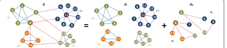
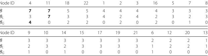
The toy example reported in Fig.1allows to illustrate the two types of influence that can occur in a modular network. For the sake of simplicity, we consider the Degree centrality measure (refer to Table1). In this case,v4andv11are the most influential nodes as they
have the highest degree value (β(v11) =β(v4) = 7). Even though they share the same degree
value the influence they have on the other nodes of the network is not comparable. Indeed, their position in the network is quite different:v11is embedded in its community, while
v4is at the border of its community. Inspecting the local and global networks give us a
clear picture of their differences. As shown in the local networkGl, nodev11is the most
influential at the community level since it is linked to all the of nodes of its community (βL(v211) = 7), while v4 is only linked to 3 nodes of its community (βL(v14) = 3). Actually,
Figure 1A toy example representing the Local network (Gl) and the Global network (Gg) associated to a
Table 1 Standard Degree centrality, Global and Local Component of the Modular Degree Centrality of the nodes in the toy example
Node ID 4 11 18 22 1 2 3 16 5 7 8
β 7 7 5 5 4 4 4 4 3 3 3
βL 3 7 3 3 4 2 4 2 3 2 3
βG 4 0 2 2 0 2 0 2 0 1 0
Node ID 9 10 14 15 17 19 21 6 12 20 13
β 3 3 3 3 3 3 3 2 2 2 1
βL 2 3 2 3 3 3 3 1 2 2 1
βG 1 0 1 0 0 0 0 1 0 0 0
both nodesv1 andv3 are more influential than nodev4in the communityC1with their
higher Local Degree values. Looking at the Global networkGg, it appears clearly than node
v4is the most influential node at the network level since it is connected to 4 nodes inside its
component (βG(v14) = 4). These nodes belong to all the other communities of the network
(C1,C2andC3). Therefore,v4is more influential than nodev11in the global networkGg
because of its ability to reach the different modules of the network as compared tov11
which is influential only locally (in the communityC2).
To sum up, it can be noticed from this example that when we consider the Degree cen-trality, the community hubs are the most influential spreaders locally due to their ability to reach a high number of nodes in their own communities. The bridges which are linked to various communities are the most influential spreaders globally as they allow to reach a high number of communities all over the network.
3.5 Modular centrality ranking strategies
In order to rank the nodes according to their centrality, it is necessary to derive a scalar value from the Modular centrality vector. To do so, we can proceed in many different ways. In order to highlight the essential features of centrality in modular networks, we choose to consider three strategies. The first two are straightforward. Indeed, a simple way to combine the components of the Modular centrality is to use the modulus and the argument of this vector. The third strategy uses more information about the community structure in order to see if this can be beneficial.
The modulusrof the modular vectorBMof a nodeviis defined by:
r(vi) =BM(vi)=
βL
vki2+βG
vqi2 k∈ {1, . . . ,m}andq∈ {1, . . . ,p} (12)
The argumentϕof the modular vectorBMof a nodeviis defined as follows:
ϕ(vi) =arctan βG(vqi)
βL(vki)
k∈ {1, . . . ,m}andq∈ {1, . . . ,p} (13)
We propose to use the tangent of the argument because it has a higher range than the argument. It is defined by:
tanϕ(vi)
=βG(v
q i) βL(vki)
Note that in these ranking strategies the information used about the community struc-ture is very limited. As we expect that integrating more knowledge about the community structure in the combination strategy of the Modular centrality components may improve the efficiency of the ranking method, we also investigate the so-called “Weighted Modular measure”. It is based on a linear combination of the components of the Modular centrality vector weighted by a measure of the strength of the communities.
The Weighted Modular measureαWof a nodeviis given by:
αW(vi) = (1 –μCk)∗βL
vki+μCk∗βG
vqi, (15)
wherek∈ {1, . . . ,m},q∈ {1, . . . ,p}and:
μCk=
vi∈Ckk inter(vk
i)
vi∈Ckk(v
k i)
, (16)
whereμCk is the fraction of inter-community links of the communityCk. kinter(vk
i) is the number of inter-community links of nodevki andk(vi) is the degree of
nodevk i.
The Weighted Modular measure works as follows:
• A communityCk, where the intra-community links predominate is densely connected
and therefore it has a very well-defined community structure. If an epidemic starts in such a cohesive community, it has more chance to stay confined than to propagate through the few links that allows to reach the other communities of the network. In this case, priority must be given to local immunization. Consequently, more weight is given to the Local component of the Modular centralityβLto target the most
influential nodes in the community since it is well separated from the other communities of the network.
• A communityCkwhere the inter-community links predominate has a non-cohesive
community structure. It is more likely that an epidemic starting in this community diffuses to the other communities through the many links that it shares with the other communities. Consequently, more weight is given to the Global component of the Modular centrality measureβGin order to target nodes that can propagate the
epidemic more easily all over the network due to the loose community structure ofCk.
4 Experimental setting
In this section, we give some information about the synthetic and real-world dataset used in the empirical evaluation of the centrality measures. The SIR simulation process is re-called, together with the measure of performance used in the experiments.
4.1 Dataset
4.1.1 Synthetic networks
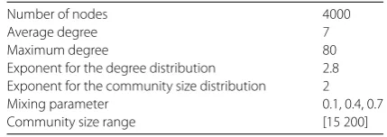
be-Table 2 LFR network parameters
Number of nodes 4000
Average degree 7
Maximum degree 80
Exponent for the degree distribution 2.8 Exponent for the community size distribution 2
Mixing parameter 0.1, 0.4, 0.7
Community size range [15 200]
tween a node and the ones located outside of its community. This parameter allows for controlling the strength of the community structure. If its value is low, there are few links between the communities and they are well separated from each other. In the following, we designate this situation as “well-defined community structure”. A high value ofμ in-dicates a very loose community structure. Indeed, in this case, a node shares more links with nodes outside its community than with nodes inside its community. Withμvalues ranging from 0.2 to 0.45, the community structure is referred as “community structure with medium cohesiveness”. Experimental studies have shown that typical value of the de-gree distribution exponent in real-world networks varies in the range 2≤γ ≤3. Networks can have different size going from tens to millions of nodes. In addition, it is also difficult to characterize the average and the maximal degree since they are very variable. Conse-quently, we choose for these parameters some consensual values while considering also the computational aspect of the simulations. They are reported in Table2.
4.1.2 Real-world networks
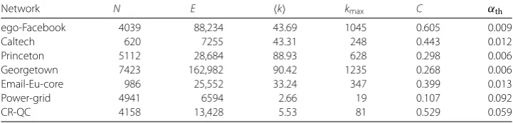
Although the LFR model produces pretty realistic networks, uncontrolled properties such as transitivity and degree correlation can deviate significantly from those observed in real-world networks [30]. Therefore, it is necessary to use real-world networks in the evaluation process. In order to cover a wide range of situations, we selected networks from various origin: online social networks, collaboration networks, technological networks, commu-nication networks. All networks are undirected and unweighted. Experiments are per-formed on their largest connected component. The Louvain Algorithm is used to unveil the community structure of these networks. We choose this greedy optimization method for its simplicity. Furthermore, this popular algorithm has proved to be a good compro-mise between efficiency and complexity when used in many different types of networks [31,32].
– Social networks:Four Samples of the Facebook Network are used. The ego-Facebook network collected from survey participants using the Facebook app. [33] and the Facebook friendship network at 3 US universities (Caltech, Princeton, Georgetown) collected by Traud et al. [34]. Nodes represent individuals (survey participant or members of the University), and edges represent online friendship links between two individuals. In the University network, in order to obtain data that are relevant for the spread of epidemic infections, only the relationship of individuals who live in the same dormitory or study the same major are considered.
Table 3 Description of the structural properties of the real-world networks.Nis the total numbers of nodes,Eis the number of edges.k,kmaxare respectively the average and the max degree.Cis the
average clustering coefficient.αthis the epidemic threshold of the network
Network N E k kmax C αth
ego-Facebook 4039 88,234 43.69 1045 0.605 0.009
Caltech 620 7255 43.31 248 0.443 0.012
Princeton 5112 28,684 88.93 628 0.298 0.006
Georgetown 7423 162,982 90.42 1235 0.268 0.006
Email-Eu-core 986 25,552 33.24 347 0.399 0.013
Power-grid 4941 6594 2.66 19 0.107 0.092
CR-QC 4158 13,428 5.53 81 0.529 0.059
– Technological network:Power-Gridbis a network containing information about the topology of the Western States Power Grid of the United States. An edge represents a power supply line. A node is either a generator, a transformer or a substation. – Collaboration network:GR-QCa(General Relativity and Quantum Cosmology)
collaboration network has been collected from the e-print arXiv and covers scientific collaborations between authors of papers submitted to the General Relativity and Quantum Cosmology category. If an authorico-authored a paper with authorj, the graph contains an edge fromitoj. If the paper is co-authored bykauthors this generates a completely connected (sub)graph onknodes.
The basic topological properties of these networks are given in Table3.
4.2 SIR simulations
To evaluate the efficiency of the centrality measures, we consider an epidemic spreading scenario using the Susceptible-Infected-Recovered (SIR) model [35]. In this setting, nodes can be classified into three classes: S (Susceptible), I (Infected) and R (Recovered). Initially, all nodes are set as susceptible nodes. Then, a given fractionf0of the top-ranked nodes
according to the centrality measure under test are set to the state infected. After this ini-tial setup, at each iteration, each infected node affects one of its susceptible neighbors with probabilityα. Besides, the infected nodes turn into recovered nodes with the recover probabilityσ. To better characterize the spreading capability, the value of the transmission rateαis chosen to be greater than the network epidemic thresholdαthgiven by [36]:
αth=
k
k2 –k , (17)
wherek andk2 are respectively the first and second moments of the degree
distribu-tion. The epidemic threshold valuesαthfor the networks used in this study are reported
in Table3. In all the experiments, we use the same value of the transmission rate (α= 0.1). Naturally, it is much larger than the values of the epidemic thresholdαthof all the dataset.
Algorithm 2:Decription of the SIR simulation process Input : GraphG(V,E),
Centrality measure:β,
Fraction of the initial spreaders:f0,
Transmission rate:α, Recovery rate:σ,
The number of simulations:n
Output: The average number of the recovered nodes after the SIR simulations:rav,
The standard deviation:rdev
1 Rank the nodes according to the centrality measureβ
2 Set all nodes as susceptible nodes
3 ComputenIthe number of initially infected nodes:nI←card(V)∗f0
4 SelectnIof the top-ranked nodes and change their state to the infected state
5 Add the initially infected nodes to the infected listL_Infected
6 Initialize the list of the numbers of recovered nodesnRobtained after each
simulation:L_nbrR←EmptyList()
7 forcounter from0to ndo
8 nR←0
9 whileL_Infected=Nulldo
10 Select one infected nodevfrom the infected listL_Infected
11 foreach node vneighbor of vdo
12 if vis susceptiblethen
13 With a probabilityαset the nodevas infected
14 L_Infected.add(v)
15 end
16 else
17 With a probabilityσset the nodevas recovered
18 L_Infected.remove(v)
19 nR←nR+ 1
20 end
21 end
22 end
23 nR←nR–nI
24 L_nbrR.add(nR)
25 end
26 Compute the average numberravand the standard deviationrdevof the recovered
nodes over thensimulations based on the listL_nbrR
27 Returnrav,rdev
4.3 Evaluation criteria
In order to compare the ranking efficiency of a centrality measure with the one obtained by a reference centrality measure, we compute the relative difference of the outbreak size. It is given by:
r=Rm–Rs
Rs
, (18)
whereRmis the final number of recovered nodes of the ranking method under test, and
Rsis the final number of recovered nodes for the reference method. Thus, a positive value
ofrindicates a higher efficiency of the method under test as compared to the reference.
5 Experimental results
Extensive experiments have been performed in order to evaluate the effectiveness of the most popular Modular centrality extensions (Degree, Betweenness, Closeness and Eigen-vector centrality) as compared to their standard definition. First, the Local and Global component of the various Modular centrality measures is compared to their standard counterpart. Next, the three ranking methods based on the combination of the compo-nents of the Modular centrality are also evaluated. These experiments are conducted on both synthetic and real-world networks.
5.1 Synthetic networks
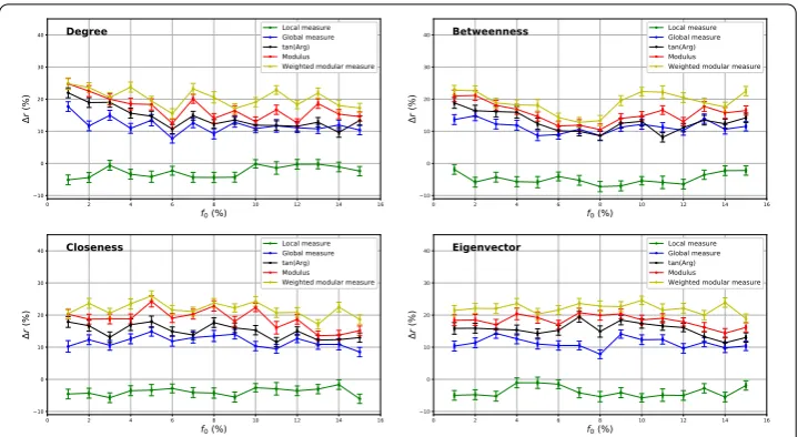
Networks with different mixing parameter values have been generated in order to better understand the effect of the community structure strength on the performance of the var-ious centrality measures. Figure2represents the relative difference of the outbreak size as a function of the fraction of immunized nodes with the standard measure used as a refer-ence. The mixing parameter valuesμcover all the range of community structure strength.
5.1.1 Evaluation of the local and the global component of the Modular centrality
a. Well-defined community structure In networks with well-defined community struc-ture, the Local component of the Modular centrality always outperforms the standard measures for all the centrality measures as it is shown in the left panels of the Fig.2(when
μ= 0.1). The gain is around 20% as compared to the standard measure for Closeness, De-gree and Eigenvector centrality. The smallest gain is for Betweenness centrality with an average value of 10%. On the contrary, the Global component of the Modular centrality is always less performing than the standard measures. These results clearly demonstrate that it is more efficient to immunize the influential nodes inside the communities when there are few inter-community links in the networks. Indeed, as there are few inter-community edges, the infection may die out before reaching other communities. So, the local influ-ence of nodes is more important than global influinflu-ence in networks with strong community structure.
Figure 2The relative difference of the outbreak sizeras a function of the fraction of the initial spreadersf0
for Synthetic networks. The Degree (a), Betweenness (b), Closeness (c) and Eigenvector (d) centrality measures derived from the Modular centrality are compared to the standard counterpart designed for networks with no community structure. Networks are generated using the LFR algorithm with variousμ values. For eachμvalue, five sample networks are generated. The final epidemic sizes are obtained by averaging 200 SIR model simulations per network for each initial spreading coverage value. Positivervalue means higher efficiency of the measure under test as compared to the standard centrality
Local component. Indeed, the Global component outperforms the standard measure with a Gain around 12% for Betweenness, Closeness and Eigenvector centrality. The largest gain is for the Degree centrality with an average value of 17%. The Local component of the Modular centrality performs better than the standard measure with a gain around 5% for Betweenness, Closeness and Eigenvector centrality and around 12% for Degree cen-trality. These results send a clear message: In networks with medium community structure strength, the global influence is more important than the local influence. Indeed, with a greater number of inter-community links, there are more options to spread the epidemics to the other communities of the network.
out-break size between the Global component of the Modular centrality and the standard cen-trality is always positive while it is always negative for the Local component of the Modular centrality. And this is true for all the centrality measures under test. In fact, there is a gain of around 5% using the Global component of the Modular centrality, while the Local com-ponent performs worse than the traditional measure with an average of 5% for the Degree, Betweenness, Closeness and Eigenvector centrality measures. Consequently, we can con-clude that in networks with a loose community structure the global influence is dominant, even if the difference with the standard measure is not as important than for networks with a medium community structure. Indeed, in this situation (μ= 0.7), the inter-community edges constitute the majority of edges in the network (around 70% of links lie between the communities). In fact, as the community structure is not well defined, minor differences are observed with a network that has no community structure.
5.1.2 Evaluation of the ranking methods of the Modular centrality
Figure2reports also the relative difference of the outbreak sizeras a function of the fraction of the initial spreadersf0for the three ranking methods (Modulus and Tangent of
become less and less important. Indeed, the global network size increases until it tends to represent the major part of the original network. In the limiting case, it is a network with no community structure and the Modular centrality reduces to its Global compo-nent which is identical to the classical centrality measures.
5.2 Real-world networks
In this section, we report the results of the set of experiments on real-world networks. Experiments performed with synthetic networks have shown that the community struc-ture strength plays a major role in determining the performance of the various centrality measures. Therefore, we adopt the same presentation for real-world networks in order to link the results of this set of experiments with those obtained using synthetic networks. Once the community structure has been uncovered using the Louvain algorithm, the mix-ing proportion parameter is computed for each network. Estimated values are reported in Table4. According to these results, we can classify the ego-Facebook network, Power Grid and the ca-GrQc as networks with strong community structure. Princeton, Email-Eu-core and Caltech have a community structure of medium strength while Princeton has a weak community structure.
5.2.1 Evaluation of the local and global component of the Modular centrality
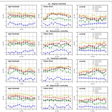
a. Well-defined community structure The relative difference of the outbreak size between the community-based measures and the standard measure is reported in Fig.3. To evaluate their performances in networks with strong community structure, ego-Facebook, power grid and the ca-GrQc networks are used. For these networks, the estimated mixing pa-rameter value ranges from 0.03 to 0.095. In this figure, we notice that for all the central-ity measures under test the standard measure outperforms the Global component of the Modular centrality while it is less performing that its Local component. Let’s consider for example the Betweenness centrality. With a fraction of the initial spreaders equal to 8%, the gain in terms of the outbreak size for the Local component of the Modular centrality as compared to the standard Betweenness is 19% for the ego-Facebook network, 14% for Power-Grid and 9% for ca-QrGc. Conversely, in the same situation, the loss associated with the use of the Global component of the Modular centrality instead of the standard Betweenness ranges from 4% to 11%.
In these networks, communities are densely connected and there are few links lying between the communities. Therefore, in most cases, contagious areas are found in the core of the communities and the spread of the epidemic may stop before even reaching the community perimeter. Thus, there is a low probability that a bridge (inter-community link) propagates the epidemic to the other communities. This is the reason why the Local
Table 4 The estimated mixing parameterμand modularityQof the real-world networks
Network ego-Facebook Power-grid ca-GrQc Princeton
μ 0.03 0.034 0.095 0.354
Q 0.834 0.934 0.86 0.753
Network Email-Eu-core Caltech Georgetown
μ 0.42 0.448 0.522
Figure 3The relative difference of the outbreak sizeras a function of the fraction of initial spreadersf0. The
Degree (a), Betweenness (b), Closeness (c) and Eigenvector (d) centrality measures derived from the Modular centrality are compared to the standard counterpart designed for networks with no community structure. Real-world networks with strong community structure (ego-Facebook, Power-Grid and ca-GrQc networks) are used. The estimated values of their mixing coefficient is equal respectively to 0.03, 0.034 and 0.095
component of the Modular centrality performs always better than the Global component. Furthermore, we can also notice on Fig.3that when the mixing parameter value increases (i.e., the community structure gets weaker), the Local component of the Modular central-ity gets less efficient while the Global component performs better. This is due to the fact that the Global component increases with the number of inter-community links.
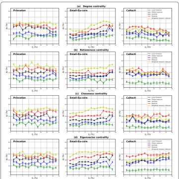
Figure 4The relative difference of the outbreak sizeras a function of the fraction of initial spreadersf0. The
Degree (a), Betweenness (b), Closeness (c) and Eigenvector (d) centrality measures derived from the Modular centrality are compared to the standard counterpart designed for networks with no community structure. Real-world networks with medium community structure (Princeton, Email-Eu-core and Caltech) are used. The estimated values of their mixing coefficient is equal respectively to 0.354, 0.42 and 0.44
Figure 5The relative difference of the outbreak sizeras a function of the fraction of initial spreadersf0. The
Degree (a), Betweenness (b), Closeness (c) and Eigenvector (d) centrality measures derived from the Modular centrality are compared to the standard counterpart designed for networks with no community structure. A real-world networks with weak community structure (Georgetown) is used. The estimated value of its mixing coefficient is equal to 0.522
c. Loose community structure Figure5shows the relative difference of the epidemic out-break size between the modular based centrality measures and the standard centrality for the Georgetown network. With a mixing parameter value equal to 0.522, this network is classified as a network with a weak community structure. In all circumstances, the stan-dard measure performs better than the Local component of the Modular centrality and it performs worse than its Global component. On average, there is a gain of around 10% for the Global component compared to a loss of 5% for the Local component of the four centrality measures under test. In this type of networks, the inter-community links pre-dominate, which translates into a greater influence of the Global component of the Mod-ular centrality. Indeed, the epidemic can spread more easily into the various communities of the network through the big amount of external links. Additionally, we notice that the relative difference of the outbreak size between the Global component of the Modular centrality measure and the standard measure decreases as compared to networks with a medium community structure. Indeed, there are less and less topological differences be-tween networks with a weak community structure and networks that have no community structure as the value of the mixing parameter increases.
5.2.2 Evaluation of the ranking methods of the Modular centrality
on Georgetown. As the ranking strategies use both the local and the global information of each node, they are more efficient than measures relying on either local or global infor-mation taken separately. Furthermore, the Weighted Modular measure is usually the most efficient measure in most cases. It uses the fraction of inter-community links as additional information to target the most influential spreaders in each community. It can give more or less weight to the Local and the Global component according to the individual com-munity structure strength. This explains its superiority over the other ranking measures. To summarize, these experiments reveal that combining the components of the Modular centrality, allows designing efficient ranking methods. In addition, using more relevant in-formation about the community structure at the community level allows designing even more efficient ranking methods. Moreover, the ranking measures exhibit their best results in networks with strong community structure.
5.2.3 Comparisons with the alternative measures
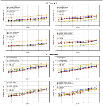
Figure6shows the average fraction of the epidemic size versus the proportion of the ini-tial spreaders for the Modular centrality components and their standard counterparts. The performance of the alternative Modular centrality measures presented in the related work section is also reported in this figure (i.e., Comm centrality, Number of Neighboring Communities NNC and Community Hub-Bridge centrality CHB). The figures report the results for the Power-grid network in (a) and the Georgetown network in (b). The former has a well-defined community structure while the latter one has a loose community struc-ture. For both networks in Fig.6(a) and (b) and for all the tested measures, one can see that increasing the proportion of the initial spreaders, the epidemic size increases as well. However, this evolution is slower in Power-grid as compared to Georgetown. Indeed, be-cause of its well-separated modules, the epidemics cannot move easily from one module to another in Power-grid.
Overall, the Betweenness-based centralities (Local, Global, Weighted Modular central-ity, Standard Betweenness) outperforms all the other alternatives. Note that, even the stan-dard Betweenness centrality is more efficient than the other alternatives. This result is independent of the community structure strength. In networks with a well-defined com-munity structure (i.e., Power-grid network), one can see on Fig.6(a) that the Eigenvector-based centralities are just below, followed by the Degree-Eigenvector-based centralities. The lowest performance is obtained by the Closeness-based centrality measures. The Comm and Number of Neighboring Communities exhibit a lower efficiency as compared to the three versions (Standard, Local and Weighted Modular measures) of the four previous central-ities. Their performance is, however, as good as the Global measures with slightly higher performance for the NNC measure. These two methods tend to target bridge nodes that have a high global influence in the network. This is the reason why they perform at the same level as global measures. Furthermore, the Community Hub-Bridge measure has globally the same performance as the Weighted Modular Betweenness. As this central-ity incorporates both local and global influence of nodes it performs better than most of the other measures. This corroborates the fact that both dimensions must be taken into account in order to design a centrality measure in modular networks.
differ-Figure 6The epidemic size as a function of the fraction of initial spreadersf0. The standard and the modular
variations of Degree, Betweenness, Closeness and Eigenvector centrality measures as well as some alternative measures (i.e., Comm, Number of Neighboring Communities and Community Hub-Bridge) are tested on two real-world networks of different community structure strength
Table 5 The estimated mixing parameterμand the modularityQin Power-grid and Georgetown networks
Network Metric Detection algorithm
Louvain Infomap
Power-grid μ 0.034 0.038
Q 0.92 0.93
Georgetown μ 0.522 0.491
Q 0.521 0.601
Figure 7The relative difference of the outbreak sizeras a function of the fraction of initial spreadersf0. The
Degree and Betweenness centrality measures derived from the Modular centrality are compared to their classical counterparts. The measures are performed on Power-grid network in (a) and Georgetown network in (b) for theInfomapalgorithm
5.2.4 Influence of the community detection algorithms
In this section, we report a set of experiments conducted on Power-grid and Georgetown networks using the Infomap algorithm [37] instead of Louvain. These two real-world net-works are chosen because of their different community structure strength. The Power-grid network has a strong community structure while Georgetown network has a non-cohesive community structure. The main purpose of these experiments is to get a clear picture of the influence of the community detection algorithm on the performance of the Modular centrality components. The estimated values of the proportion of inter-community links and the modularity for both Infomap and Louvain algorithms are reported in Table5.
propor-tions of the initial seeds. Additionally, the overall gain of the Weighted Modular measure is around 45% and 42% for Degree and Betweenness measures when using Infomap, while it is around 40% for both centrality measures when Louvain algorithm is employed. Thus, the Modular centrality extensions display a slightly better performance for the Infomap al-gorithm. Indeed, Infomap and Louvain detection algorithms have nearly the same mixing parameter and modularity measures. Therefore, in networks with a well-defined commu-nity structure, both commucommu-nity detection algorithms uncover about the same commucommu-nity structure. Consequently, the performance of the Modular centrality display roughly the same behavior.
In networks with a loose community structure (e.g., Georgetown network), the stan-dard measure is always better performing than the Local measure. The Global measure, however, performs better than the Standard one with an average gain of 17% and 16% for the Degree and Betweenness centrality measures respectively. Whereas the average gain is around 11% in the case of Louvain algorithm for both centrality measures. On the other hand, the overall gain of the Weighted Modular measure is around 29% and 25% for Degree and Betweenness measures when using Infomap, while it is around 20% and 19% for both centrality measures respectively when Louvain algorithm is employed. In this network, the Infomap algorithm has a relatively smaller mixing parameter and higher modularity. Infomap is then more accurate as compared to Louvain algorithm. That ex-plains why the performance of the Modular centrality components enhances in networks with a non-cohesive community structure when the Infomap detection algorithm is used. Globally, the results of this set of experiments show that variations of the uncovered community structure impact the performance of the centrality measures. The efficiency of the measures increases with the modularity of the community structure.
6 Conclusion
weak community structure the Global component performs better than its alternatives. Moreover, it is also observed that combining both components of the Modular centrality in order to rank the nodes according to their influence is always more efficient than to use a single component. Furthermore, a further gain can be obtained if the ranking strategy in-corporates more information about community structure strength. We perform also a set of experiments using the Infomap detection algorithm to uncover communities. Results show that the performance of the Modular centrality variants exhibit the same behavior in networks with a well-defined community structure. Their performance, however, is dif-ferent in networks with a loose community structure. In this case, slightly better results are obtained with the Infomap algorithm.
Acknowledgements Not applicable.
Funding Not applicable.
Abbreviations
SIR, Susceptible-Infected-Recovered; LFR, Lancichinetti–Fortunato–Radicchi benchmark; GR-QC, General Relativity on Quantum Cosmology.
Availability of data and materials
The datasets used in this article are all publicly available and cited in the references.
Competing interests
The authors declare that they have no competing interests.
Authors’ contributions
All the authors contributed to designing the proposed method. ZG implemented the model and all the analyses. All authors participated in the formulation and writing of this paper. All authors approved the final manuscript.
Author details
1LRIT URAC No 29, Faculty of Science, Rabat IT Center, Mohammed V University, Rabat, Morocco.2DISP Lab, University of
Lyon 2, Lyon, France. 3LE2I, UMR6306 CNRS, University of Burgundy, Dijon, France.
Endnotes
a http://snap.stanford.edu/data
b http://www-personal.umich.edu/~mejn/netdata/
Publisher’s Note
Springer Nature remains neutral with regard to jurisdictional claims in published maps and institutional affiliations.
Received: 13 July 2018 Accepted: 30 April 2019
References
1. Wang Z, Moreno Y, Boccaletti S, Perc M (2017) Vaccination and epidemics in networked populations—an introduction. Chaos Solitons Fractals 103:177–183
2. Medo M, Zhang Y-C, Zhou T (2009) Adaptive model for recommendation of news. Europhys Lett 88(3):38005 3. Zhang Z-K, Liu C, Zhan X-X, Lu X, Zhang C-X, Zhang Y-C (2016) Dynamics of information diffusion and its applications
on complex networks. Phys Rep 651:1–34
4. Coscia M, Giannotti F, Pedreschi D (2011) A classification for community discovery methods in complex networks. Stat Anal Data Min ASA Data Sci J 4(5):512–546
5. Cherifi H (2014) Chapter eleven. Non-overlapping community detection. In: Complex networks and their applications, p 320
6. Fortunato S, Hric D (2016) Community detection in networks: a user guide. Phys Rep 659:1–44
7. Jebabli M, Cherifi H, Cherifi C, Hamouda A (2015) User and group networks on YouTube: a comparative analysis. In: Computer systems and applications (AICCSA), 2015 IEEE/ACS 12th international conference of. IEEE, pp 1–8 8. Jebabli M, Cherifi H, Cherifi C, Hammouda A (2014) Overlapping community structure in co-authorship networks: a
case study. In: u- and e-service, science and technology (UNESST), 2014 7th international conference on. IEEE, pp 26–29
9. Palla G, Derényi I, Farkas I, Vicsek T (2005) Uncovering the overlapping community structure of complex networks in nature and society. Nature 435(7043):814
11. Kumar M, Singh A, Cherifi H (2018) An efficient immunization strategy using overlapping nodes and its neighborhoods. In: International World Wide Web Conferences Steering Committee, pp 1269–1275
12. Chakraborty D, Singh A, Cherifi H (2016) Immunization strategies based on the overlapping nodes in networks with community structure. In: International conference on computational social networks. Springer, Berlin, pp 62–73 13. Taghavian F, Salehi M, Teimouri M (2017) A local immunization strategy for networks with overlapping community
structure. Phys A, Stat Mech Appl 467:148–156
14. Lü L, Chen D, Ren X-L, Zhang Q-M, Zhang Y-C, Zhou T (2016) Vital nodes identification in complex networks. Phys Rep 650:1–63
15. Ferrara E, De Meo P, Fiumara G, Provetti A (2012) The role of strong and weak ties in Facebook: a community structure perspective. ArXiv preprintarXiv:1203.0535
16. Granovetter MS (1973) The strength of weak ties. Am J Sociol 78:1360–1380
17. Salathé M, Jones JH (2010) Dynamics and control of diseases in networks with community structure. PLoS Comput Biol 6(4):e1000736
18. Gupta N, Singh A, Cherifi H (2015) Community-based immunization strategies for epidemic control. In: Communication systems and networks (COMSNETS), 2015 7th international conference on. IEEE, pp 1–6 19. Gong K, Tang M, Hui PM, Zhang HF, Younghae D, Lai Y-C (2013) An efficient immunization strategy for community
networks. PLoS ONE 8(12):e83489
20. Zhao Z, Wang X, Zhang W, Zhu Z (2015) A community-based approach to identifying influential spreaders. Entropy 17(4):2228–2252
21. Nadini M, Sun K, Ubaldi E, Starnini M, Rizzo A, Perra N (2018) Epidemic spreading in modular time-varying networks. Sci Rep 8(1):2352
22. Chan SY, Leung IX, Liò P (2009) Fast centrality approximation in modular networks. In: Proceedings of the 1st ACM international workshop on complex networks meet information & knowledge management. ACM, New York, pp 31–38
23. Yoshida T, Yamada Y (2017) A community structure-based approach for network immunization. Comput Intell 33(1):77–98
24. Newman ME (2006) Finding community structure in networks using the eigenvectors of matrices. Phys Rev E 74(3):036104
25. Gupta N, Singh A, Cherifi H (2016) Centrality measures for networks with community structure. Phys A, Stat Mech Appl 452:46–59
26. Ghalmane Z, Hassouni ME, Cherifi H (2018) Immunization of networks with non-overlapping community structure. ArXiv preprintarXiv:1806.05637
27. Luo S-L, Gong K, Kang L (2016) Identifying influential spreaders of epidemics on community networks. ArXiv preprint
arXiv:1601.07700
28. Kitromilidis M, Evans TS (2018) Community detection with metadata in a network of biographies of western art painters. ArXiv preprintarXiv:1802.07985
29. Lancichinetti A, Fortunato S, Radicchi F (2008) Benchmark graphs for testing community detection algorithms. Phys Rev E 78(4):046110
30. Orman GK, Labatut V, Cherifi H (2013) Towards realistic artificial benchmark for community detection algorithms evaluation. Int J Web Based Communities 9(3):349–370
31. Orman GK, Labatut V, Cherifi H (2011) On accuracy of community structure discovery algorithms. ArXiv preprint
arXiv:1112.4134
32. Orman GK, Labatut V, Cherifi H (2012) Comparative evaluation of community detection algorithms: a topological approach. J Stat Mech Theory Exp 2012(08):P08001
33. Leskovec J, Mcauley JJ (2012) Learning to discover social circles in ego networks. In: Advances in neural information processing systems, pp 539–547
34. Traud AL, Mucha PJ, Porter MA (2012) Social structure of Facebook networks. Phys A, Stat Mech Appl 391(16):4165–4180
35. Moreno Y, Pastor-Satorras R, Vespignani A (2002) Epidemic outbreaks in complex heterogeneous networks. Eur Phys J B, Condens Matter Complex Syst 26(4):521–529
36. Wang W, Liu Q-H, Zhong L-F, Tang M, Gao H, Stanley HE (2016) Predicting the epidemic threshold of the susceptible-infected-recovered model. Sci Rep 6:24676