Gyrokinetic Vlasov Code Including Full Three-dimensional
Geometry of Experiments
Masanori NUNAMI
1), Tomo-Hiko WATANABE
1,2)and Hideo SUGAMA
1,2) 1)National Institute for Fusion Science, Toki 509-5292, Japan2)The Graduate University for Advanced Studies (SOKENDAI), Toki 509-5292, Japan
(Received 23 February 2010/Accepted 17 March 2010)
A new gyrokinetic Vlasov simulation code, GKV-X, is developed for investigating the turbulent transport in magnetic confinement devices with non-axisymmetric configurations. Effects of the magnetic surface shapes in three-dimensional equilibrium obtained from the VMEC code are accurately incorporated. Linear simulations of ion temperature gradient (ITG) instabilities and zonal flows in the Large Helical Device (LHD) [O. Motojima, N. Oyabu, A. Komoriet al., Nucl. Fusion43, 1674 (2003)] configuration are carried out by the GKV-X code as benchmark tests against the GKV code [T.-H. Watanabe and H. Sugama, Nucl. Fusion46, 24 (2006)]. For high poloidal wavenumbers, the frequency, growth rate, and mode structure of the ITG instability are influenced by the VMEC geometrical data such as the metric tensor components of the Boozer coordinates, while the difference between the zonal flow responses obtained by the GKV and GKV-X codes is found to be small in the core LHD region.
c
2010 The Japan Society of Plasma Science and Nuclear Fusion Research
Keywords: gyrokinetic simulation, ITG mode, zonal flow, LHD, VMEC equilibrium DOI: 10.1585/pfr.5.016
1. Introduction
Anomalous transport of particles, momentum, and heat is commonly observed in fusion plasma experiments, and has been a central issue in magnetic fusion research for the last few decades. The anomalous transport is consid-ered to be driven by the drift-wave plasma turbulence [1], e.g., the ion temperature gradient (ITG) turbulence. The zonal flows are known to play a critical role in regulat-ing the turbulent transport in toroidal plasmas, and various studies on the zonal flows have been conducted for toka-maks and stellarator/heliotron configurations [2–4].
To explore the zonal flow and microturbulence in axisymmetric configurations, a number of linear and non-linear gyrokinetic simulations have been performed [5–9]. In our previous studies [6, 10], we investigated the effects of single and multiple helicity magnetic field configura-tions on the ITG turbulence in the helical system using the gyrokinetic Vlasov flux-tube code, GKV [11]. The simulation results indicate that a neoclassically optimized (inward-shifted) helical configuration causes a reduction in the ion heat transport through the enhancement of the zonal flows as compared with that in the standard configu-ration. This is also qualitatively consistent with the Large Helical Device (LHD) [12] experimental results, which in-dicate that the anomalous transport in the inward-shifted cases is reduced with a decrease in the radial drift of ripple-trapped particles [13], but with an increase in the unfavor-able field line curvature [14].
author’s e-mail: [email protected]
To understand anomalous transport physics better, quantitative comparisons between the gyrokinetic tions and experiments are required. In the GKV simula-tions, the model helical fields including limited number of helical Fourier components are employed with the large aspect ratio approximation to the field geometry, where the Jacobian is assumed to be a constant on the flux sur-face, and diagonal metric tensor components derived from the cylindrical approximation are used. For more quantita-tive gyrokinetic simulations, it is a natural path to furnish a well-established gyrokinetic code with detailed geomet-rical information obtained from three-dimensional equilib-rium calculations as in Refs. [15–17]. Based on this mo-tivation, we developed a new gyrokinetic Vlasov code, GKV-X. The GKV-X code precisely deals with realistic magnetic configurations, using all the geometrical infor-mation provided by the VMEC code [18], which is a stan-dard magnetohydrodynamic equilibrium solver for non-axisymmetric systems. Using the GKV-X code, we inves-tigate the effects of full geometry of the LHD plasmas on the linear ITG mode and the zonal flow response [6,19–23] by the benchmark tests against the GKV calculation.
The rest of this paper is organized as follows. In Sec. 2, we summarize the field representation and geom-etry in flux coordinate system. In Sec. 3, we describe basic equations employed in the GKV and GKV-X codes, and clarify the differences between the codes for concrete rep-resentations of each term in the equations. In Sec. 4, sim-ulation results of the linear ITG instability and the zonal flow response are compared for both the codes to
inves-c
tigate the effects of the metric tensor and the Jacobian in helical systems. Section 5 presents the conclusions of the study.
2. Magnetic Field Geometry
The detailed expressions of the magnetic field rep-resentation and geometry in the flux coordinate system are described here. We consider the flux coordinate sys-tem{ρ, θ, ζ}, whereθandζ are poloidal and toroidal an-gles, respectively. The labeling index of the flux surfaces,
ρ ≡ √Ψ/Ψa, is a dimensionless quantity. HereΨ
repre-sents the toroidal magnetic flux with the minor radius,r, defined byΨ =Baxr2/2, with a field strength at the mag-netic axis,Bax, and Ψa is the value of the toroidal flux at
the last closed surface. Therefore, the flux label can be rep-resented asρ=r/a, whereadenotes the minor radius of the last closed surface defined byΨa=Baxa2/2 atρ=1.
2.1
Field representation
Let us consider the Boozer coordinates [24]{ρ, θB, ζB} as the flux coordinate system. The contravariant represen-tation of the magnetic field in the Boozer coordinates, is written as
B=∇Ψ(ρ)× ∇θB+q−1(ρ)∇ζB× ∇Ψ(ρ) = √Ψg
B
eζB+q− 1(ρ)e
θB
=BζBe ζB+B
θBe
θB, (1)
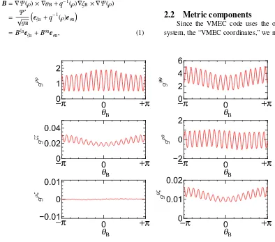
Fig. 1 Example of contravariant components of metric tensor, used fork⊥ in Eq. (26), obtained by the VMEC/NEWBOZ outputted configuration atρ=0.6 in the Boozer coordinate system{ρ, θB, ζB}with a fixedα=ζB−q0θB. Each component is in units ofa−2.
where,eθB ≡∂r/∂θB,eζB ≡∂r/∂ζB,q(ρ) is the safety factor and √gBis the Jacobian in the coordinate system,
√g
B=(∇ρ× ∇θB· ∇ζB)−1 =Ψ
B2
BζB+q− 1(ρ)B
θB
, (2)
where the prime symbol represents the derivative with re-spect to the flux labelρ, i.e., A = dA/dρ. Hereafter, for the sake of simplicity, the subscript “B” of the poloidal and toroidal angles is omitted when the angles are used as sub-scripts of any variables, e.g.,BθB is represented asBθ. The poloidal and toroidal covariant components of the field,Bθ andBζ, are flux functions in the Boozer coordinates and consist of the covariant representation of the field written as
B=Bρ∇ρ+Bθ∇θB+Bζ∇ζB. (3)
The components of the equilibrium fieldBθ,Bζ, Bθ, and
Bζ are directly given by the VMEC code except for the component Bρ. The radial covariant component, Bρ, can be determined using the contravariant components,
Bρ=Bθgθρ+Bζgζρ. (4) Here,gθρandgζρare the covariant components of the met-ric tensor.
2.2
Metric components
coordinates into the Boozer coordinates; thus, we use the NEWBOZ code [25], which transforms coordinates from the VMEC to the Boozer coordinates{ρ, θB, ζB}with the radial flux labelρ. The VMEC/NEWBOZ code package provides information about the shapes of the flux surfaces defined in the cylindrical coordinates{R,Z, φ} as Fourier series forθBandζB,
R=
k
Rk(ρ) cos(nkζB−mkθB), (5a)
Z=
k
Zk(ρ) sin(nkζB−mkθB), (5b)
φ=ζB+
k
φk(ρ) sin(nkζB−mkθB). (5c)
From Eq. (5), the covariant metric components can be ob-tained as follows:
gi j=
∂R
∂i
∂R
∂j +
∂Z
∂i
∂Z
∂j +R
2∂φ
∂i
∂φ
∂j, (6)
wherei,j={ρ, θB, ζB}. Using Eqs. (1), (2) and (3),gθζ and
gζζ can also be represented as
gθζ= √g
B
Ψ Bθ−q−1(ρ)gθθ, (7a)
gζζ = √g
B
Ψ Bζ −q−1(ρ)gθζ, (7b) which are useful for a consistency check on the calculation of the metric tensor. We can obtain the contravariant metric components from the covariant ones as given below:
gil= 1
gB
gjmgkn−gjngkm
, (8)
where {i,j,k} and {l,m,n} are even permutations of {ρ, θB, ζB}. As an example, Fig. 1 shows the contravari-ant components of the metric tensor in the standard LHD equilibrium at the flux labelρ =0.6, wheregi j fori,j =
{ρ, θB, ζB}, calculated from the VMEC/NEWBOZ output, are plotted along the field line.
3. GKV and GKV-X Codes
In this section, we present the gyrokinetic equation employed in the GKV and GKV-X codes as well as con-crete expressions of each term in which profiles along the field line are compared for both the codes.
3.1
Basic equations
Let {r, θ, ζ} be a generalized flux coordinate system. The local flux-tube model [26] with the field-aligned co-ordinates{x, y,z}is used in the codes, wherex = r−r0,
y = (r0/q0)q(ρ)θ−ζandz = θ, with the safety factor
q0 at the minor radiusr0 = ρ0a. The minor radius,r0, is defined by the toroidal magnetic fluxΨ(r=r0)=Baxr20/2. Both the codes solve the electrostatic gyrokinetic equa-tion of the perturbed ion gyrocenter distribuequa-tion funcequa-tion
δf[11, 27],
∂δf
∂t +v||b· ∇δf+ c B0
b× ∇Φ· ∇δf
+ud· ∇δf− μ mi
b· ∇B∂δf
∂v||
=u∗−ud−v||b·e∇Φ
Ti
FM+C(δf), (9) whereb = B/Bis the unit vector parallel to the magnetic field, andv|| andμ = miv2⊥/2B, regarded as the velocity-space coordinates in the codes, denote the parallel velocity and magnetic moment, respectively. The Maxwellian dis-tribution with temperatureTiand the collision term are de-noted byFM andC(δf), respectively. The magnetic drift velocity isud = (c/eB)b ×(μ∇B+miv2b· ∇b) and the diamagnetic drift velocity isu∗ = (cTi/eB)b×[∇lnn+ (miv2/2Ti−3/2)∇lnTi]. The perpendicular wavenumber vector is defined by
k⊥=kx∇r+ky∇
r0
q0
(q(r)θ−ζ)
. (10)
In the wavenumber space, (kx,ky), the average
elec-trostatic potential at the gyrocenter, Φ, is related to the electrostatic potential at the particle position, φ, as
Φkx,ky = J0(k⊥v⊥/Ωi)φkx,ky. The zeroth-order Bessel
func-tion, J0(k⊥v⊥/Ωi), represents the finite gyroradius effect, where the ion gyro frequency is defined byΩi =eB/mic. The electrostatic potential φkx,ky is calculated from the
quasi-neutrality condition
d3vJ0δfkx,ky−n0
eφkx,ky
Ti
[1−Γ0(b)]=ne,kx,ky,
(11) where δfkx,ky is the Fourier component of δf, Γ0(b) =
ebI
0(b), withb=(k⊥vti/Ωi)2, andI0is the modified zeroth-order Bessel function. The ion thermal speed is defined by
vti= √
Ti/mi. The electron density perturbation,ne,kx,ky, is
assumed to be adiabatic and is given in terms of the elec-tron temperature,Te, and the averaged density,n0, as
ne,kx,ky
n0
=⎧⎪⎪⎨⎪⎪⎩ e
φkx,ky− φkx,ky
/Te ifky=0,
eφkx,ky/Te ifky0. (12) Also,· · · indicates the flux surface average defined as
A(z)= ∞
−∞ √g
FA(z)dz ∞
−∞ √g
Fdz, (13) for an arbitrary function ofz,A(z). Here, √gF is the Ja-cobian in the coordinate system{x, y,z}, which is related
to the Jacobian in the Boozer coordinates, as shown in Eq. (2):
√g F=
q0
ar0 √g
B. (14)
We adopt the modified periodic boundary condition at the boundaries of the flux-tube domain [26]. In linear and collisionless case, the Fourier transformed expression of Eq. (9) becomes
∂
∂t +vb· ∇ −
μ
mi
b· ∇B∂v∂ +iωDi
=FM(−v b· ∇ −iωDi+iω∗Ti)J0(k⊥ρi)
eφkx,ky
Ti
, (15) whereωDi = k⊥·ud andω∗Ti = k⊥·u∗ are the magnetic and diamagnetic drift frequencies, respectively, and the ion gyroradius is defined byρi=v⊥/Ωi.
3.2
Geometrical expressions used in GKV
In the GKV simulations for helical configurations such as the LHD, we employed a model field configura-tion,
B=B0
⎡ ⎢⎢⎢⎢⎢
⎢⎣1−00(r)−t(r) cosθ−
L+1
l=L−1
l(r) cos
lθ−Mζ ⎤ ⎥⎥⎥⎥⎥ ⎥⎦,
(16) which includes the toroidalt, the main helicityh = L,
and two side-band helical components + = L+1 and
− =L−1. Here, MandLindicate the main period
num-bers of the confinement field in the toroidal and poloidal directions, respectively. For the LHD,L=2 andM =10. Here, we regard the poloidal angleθas a coordinate along the field line labeled byα = ζ−q0θ = constant. In the GKV code, we use the large aspect ratio approximation for the confinement field geometry assuming the presence of small helical ripples and cylindrical diagonal metric ten-sor [7, 8]. Under the approximation, in terms of the field-aligned coordinates{x, y,z}, the magnetic drift frequency
on the right-hand side of Eq. (15) is given by
ωDi=−
c e
μ+ 1
Bmiv
2 t r0 ⎡ ⎢⎢⎢⎢⎢ ⎢⎣ky
⎛ ⎜⎜⎜⎜⎜ ⎜⎝ρ0
00
t +
ρ0t
t cosz
+
L+1
l=L−1
ρ0l
t
cos[(l−Mq0)z−Mα]
⎞ ⎟⎟⎟⎟⎟ ⎟⎠
+kx+szkˆ y
⎛⎜⎜⎜⎜⎜ ⎜⎝sinz+
L+1
l=L−1
ll
t
sin[(l−Mq0)z−Mα]
⎞ ⎟⎟⎟⎟⎟ ⎟⎠ ⎤ ⎥⎥⎥⎥⎥ ⎥⎦, (17) using Eq. (16) for a fixedα. Here, ˆs = (r0/q0)dq/dr = (ρ0/q0)qis the magnetic shear parameter and is assumed to be constant, and=d/dρ=a(d(r)/dr). The diamag-netic drift frequency is expressed as
ω∗Ti=−
cTi
eB0Ln
ky 1+ηi
miv2
2Ti − 3 2
, (18)
where ηi = Ln/LT with the background gradients for
density L−1
n = −d lnn/dr, and for temperature L−T1 =
−d lnTi/dr. The perpendicular wavenumberk⊥is written as
k2⊥=kx+szkˆ y
2
+k2y, (19) which is used for the zeroth-order Bessel function in Eq. (15) and the zeroth-order modified Bessel function in Eq. (11). The parallel derivative in Eq. (15) is given by
b· ∇= 1
R0q0
∂
∂z, (20)
where the safety factor,q0, and the major radius,R0, are re-garded as constant. This corresponds to the approximation that the Jacobian is expressed as √gF∝1/(B· ∇θ)∝1/B, i.e., B√gF is a constant on the flux surface. This im-plies that the coordinates in this model do not coincide exactly with the Boozer coordinates. In the large aspect ratio approximation, however, the difference is negligible. The flux surface average for the arbitrary function,A(z), in Eq. (13) reduces to
A(z)=
∞
−∞A(z)dz/B ∞
−∞dz/B, (21) which guarantees the propertyB· ∇A = 0. According to the approximation, the parallel derivative ofB, which is employed for the mirror force term in Eq. (15), can be written as
b· ∇B
= B0t
R0q0
⎛ ⎜⎜⎜⎜⎜ ⎜⎝sinz+
L+1
l=L−1
(l−Mq0)
l
t
sin[(l−Mq0)z−Mα]
⎞ ⎟⎟⎟⎟⎟ ⎟⎠,
(22) with the constant field line labelα.
3.3
Geometrical expressions used in GKV-X
In the GKV-X code, we employ the same basic equa-tions as that in the GKV code, i.e., Eqs. (9) and (11), but using the confinement field model obtained by the VMEC/NEWBOZ code package that gives an output of the confinement field strength in terms of the Fourier series in the Boozer coordinate system{ρ, θB, ζB}as follows:
B=
nmax
n=0
B0,n(ρ) cosnζB
+
mmax
m=1
nmax
n=−nmax
Bm,n(ρ) cos[mθB−nζB], (23)
whereBm,n(ρ) is the Fourier component with the poloidal
(m) and toroidal (n) mode numbers. Here, mmax and
nmaxare the maximum mode numbers for the poloidal and toroidal directions used in the VMEC calculation, respec-tively. Furthermore, in the GKV-X, we implement exact representations of each term in Eq. (9) with full geometri-cal factors, the Jacobian and the metric tensor. In the coor-dinates{ρ, θB, ζB}, the magnetic drift frequency in Eq. (15) with zero-beta,b· ∇b=(∇⊥B)/B, is given by
ωDi=−
c eB2 a √g B
μ+1
Bmiv
2
ky ρ0
q0
Bρ+sˆθBBζ
∂ B
∂θB
+ρ0Bρ−sˆθBBθ
∂B
∂ζB −
ρ
0
q0
Bθ+ρ0Bζ
∂ B
∂ρ
+kx Bζ∂θ∂B B
−Bθ∂ζ∂B B
, (24)
with the perpendicular wavenumbers,kxandky, where the
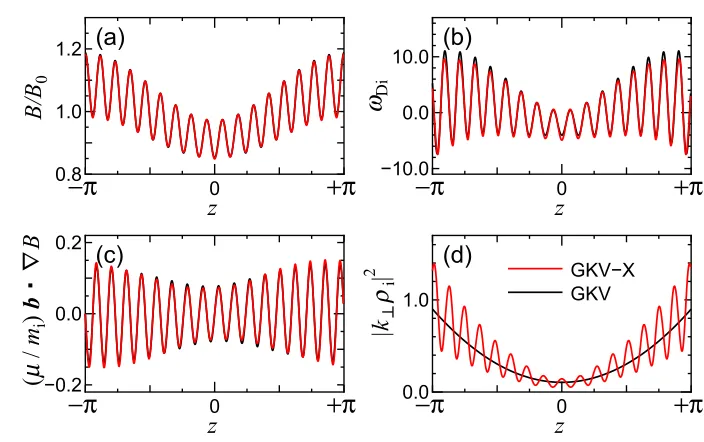
Fig. 2 Profiles of (a) normalized magnetic field strengthB/B0, (b) magnetic drift frequencyωDinormalized byvtiL−n1, (c) mirror force term normalized byv2
tiL− 1
n , and (d) square of the normalized perpendicular wavenumber,k⊥ρi. All profiles are evaluated atρ=0.6,
and three plots except for (a) are calculated forkxρi=0 andkyρi =0.324. In (b) and (c), the magnetic moment isμ/(miΩiB−1)=
0.50vtiLn. Black and red curves show the results of the GKV and GKV-X codes, respectively.
defined later. The diamagnetic drift frequency can also be expressed as
ω∗Ti=−
cTi
eLn
ρ0a2
q0B2√gB
Bθ+q0Bζ
ky 1+ηi
miv2
2Ti −3
2
=−cTi
eLn
ρ0a2
Ψ ky 1+ηi
miv2
2Ti − 3 2
, (25)
where we use Eq. (2) in the last line. Using the identity for the contravariant components of the metric tensor (Eq. (8)), we can obtain the perpendicular wavenumber k⊥ as fol-lows:
k2⊥ =k2xa2g
ρρ+
2kxkya2 sˆθBgρρ+
ρ0
q0
q0gρθ−gρζ
+k2ya2
⎡ ⎢⎢⎢⎢⎣ρ2
0
q20
gζζ+q2 0g
θθ−2q 0gθζ
+2 ˆsθB
ρ0
q0
q0gρθ−gρζ
+sˆ2θB2gρρ
. (26)
The parallel derivative is given as
b· ∇= Ψ
q0B√gB
∂
∂θB +
q0
∂ ∂ζB
, (27)
with the Jacobian Eq. (2). Therefore, in the GKV-X code, we use Eq. (13) as the flux surface averaging, and the par-allel derivative ofBcan be represented as
b· ∇B
= Ψ
q0B√gB
mmax
m=1
nmax
n=nmax
Bm,n(ρ)(m−nq0) sin[nζB−mθB]. (28)
For the benefit of comparing the magnetic drift frequencies (Eqs. (17) and (24)), we write down the concrete forms of the derivatives of the field strength along each direction in the coordinates{ρ, θB, ζB}as follows:
∂B
∂ρ =
nmax
n=0
B0,n(ρ) cosnζB
+
mmax
m=1
nmax
n=−nmax
Bm,n(ρ) cos[mθB−nζB], (29a)
∂B
∂θB =−
mmax
m=1
nmax
n=−nmax
Bm,n(ρ)m sin[mθB−nζB],(29b)
∂B
∂ζB =−
nmax
n=0
B0,n(ρ)n sinnζB
+
mmax
m=1
nmax
n=−nmax
Bm,n(ρ)n sin[mθB−nζB].(29c)
In the GKV-X code, we use the above mentioned terms after converting the coordinates into the field-aligned co-ordinates{x, y,z}with the relations, x = a(ρ−ρ0),y = (aρ0/q0)(qθB−ζB), andz= θBin a constant field line la-belα=ζB−q0θB. The parallel derivative in Eq. (27), for example, is written as b· ∇ = (Ψ/q0B√gB)(∂/∂z). The concrete profiles of each term in Eq. (15), which are used in the GKV and GKV-X simulations, are shown in Fig. 2. The profiles are discussed in detail in the following section.
4. Comparison of Simulation Results
Table 1 Parameters at flux surfaceρ=0.6 employed in the GKV code. The prime symbol indicatesA=dA/dρ.
q0 r0/R0 t h/t −/t +/t 1.9 0.0907 0.0878 0.9113 -0.2806 0.0498
ˆ
s ρ000 /t ρ0t/t ρ0h/t ρ0−/t ρ0+/t -0.87501 0.1997 1.006 1.9486 -0.6452 0.070
GKV codes are performed in a way similar to that in Refs. [7] and [11]. Here, we use the magnetic configura-tion with the parameters of the confinement field based on the VMEC calculation results for the standard LHD case, which is similar to the “S-B case” in Ref. [8]. In the GKV-X simulation, we use the VMEC configuration with full helical components. On the other hand, the GKV calcu-lation uses the parameters summarized in Table 1, which are obtained from the VMEC configuration in terms of the toroidal, main helical, two side-band components, and their radial derivatives. In both the calculations, we use the same parameters for the variables,ηi = 3,Te/Ti =1,
Ln/R0=0.3,q0=1.9, ˆs=−0.87501, andα=0.
4.1
E
ff
ects of full geometry
To highlight the differences in the effects of the metric tensor, Jacobian, and full Fourier components of the con-finement field between the two models, we plot profiles of each term in Eq. (15), concrete expressions of which were described in the previous section. In Fig. 2, we plot the nor-malized field strength; the magnetic drift frequency,ωDi, normalized byvtiL−n1; the mirror force term, (μ/mi)b· ∇B, normalized by v2
tiL− 1
n ; and the square of the normalized
perpendicular wavenumber,k⊥ρi, as functions of the field-aligned coordinatezatρ=0.6. Here, to normalize the field strength, we useB0,0(ρ) as the normalization factorB0. As seen in the figures, the profiles of the field strength, mag-netic drift frequency, and mirror force term for the GKV-X and GKV codes appear similar to each other. However, in the region nearz = 0, where the ITG instabilities are stronger because of more unfavorable magnetic field line curvature, a difference in the magnitude of the magnetic drift frequencies is not negligible and in fact, causes a dif-ference in the ITG-mode growth rates. For the diamag-netic drift frequency given in Eqs. (18) and (25), we ob-serve that there is only a small difference by the factor of
ω(GKV) ∗Ti /ω
(GKV-X)
∗Ti = Ψ/(a 2ρ
0B0)1.0097.The profiles of the perpendicular wavenumber show a clear difference due to the effects of the helical ripples on the metric tensor. In the following simulations for the linear ITG modes and collisionless damping of the zonal flows, we obtain the re-sults atρ=0.6, which is in the core plasma region of the LHD.
4.2
Linear ITG instability
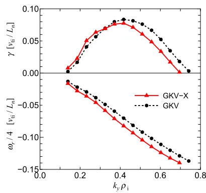
Figure 3 shows the growth rates and real frequencies
Fig. 3 Growth rates γ(top) and real frequencies ωr (bottom)
of the linear ITG mode, as functions of the normal-ized poloidal wavenumber,kyρi, for the GKV simulation
(black dashed lines with circles) and the GKV-X simula-tion (red solid lines with triangles).
of the linear ITG instability, obtained from the GKV-X and GKV simulations forρ=0.6, as functions of the normal-ized poloidal wavenumber,kyρi, wherekx=0 is used. The
growth rate in the GKV-X calculation, compared to that in the GKV, is slightly higher forkyρi <∼ 0.3 and lower for
kyρi >∼ 0.3. The real frequency obtained by the GKV-X simulation is slightly more negative than that by the GKV simulation. The differences between the codes are magni-fied with the increasing poloidal wavenumber, which orig-inates from the ripple components and full metric tensor through the magnetic drift frequency (ωDi) and perpendic-ular wavenumber (k⊥), respectively. Because more helical ripple components are included in the magnetic drift fre-quency for the GKV-X case, the difference ofωDiappears as shown in Fig. 2-(b); that is,ωDifor the GKV-X is more negative than for the GKV aroundz 0, where the ITG instabilities are strongly driven by unfavorable magnetic field line curvature. According to Eq. (24), the difference inωDiis enhanced in the large|ky|region. In the expression of the perpendicular wavenumber (Eq. (26)), the terms in-cluding the metric tensor componentsgθθ andgρρ, which reflect the shape of the elliptic magnetic surface, are influ-ential ink⊥related to the finite gyroradius effect. The term
withgθθ remains finite around z 0, and the contribu-tion of the term tok⊥ is also enhanced for higher poloidal wavenumbers, while the term withgρρvanishes atz =0. In the other terms of Eq. (15), i.e., the diamagnetic drift frequency and the mirror force term, the differences be-tween the codes are much smaller than those inωDi and
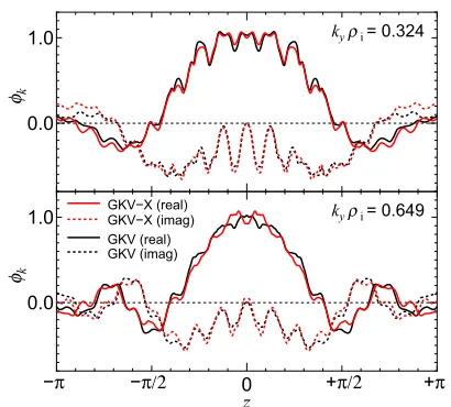
Fig. 4 Eigenfunctions of electrostatic potentialφk = φr +iφi
along the parallel-to-field coordinate z for linear ITG modes forkyρi =0.324 (top) andkyρi =0.649 (bottom)
atkx=0. Real and imaginary parts of the eigenfunctions are plotted by solid and dashed curves, respectively. Red and black curves express the results of the GKV-X and GKV codes, respectively.
drift frequency and the finite gyroradius effect.
Eigenfunctions of the ITG modes are also investigated (Fig. 4) forkyρi =0.324 andkyρi =0.649. As seen in the plot forkyρi = 0.324, the mode structures ofφk obtained
by the two codes have a similar profile, which is accompa-nied by oscillations associated with the helical ripples. In contrast, the field-aligned profiles ofφkfor larger poloidal
wavenumberkyρi =0.649 show different ripple structures in the unfavorable curvature region aroundz0. This is consistent with the results of the growth rate and the real frequency shown in Fig. 3, where the differences are found mainly in the higher poloidal wavenumbers. Linear eigen-value analysis [28–30] also predicts a similar mode struc-ture to the present results.
4.3
Zonal flow evolution
The zonal flows are produced by an electrostatic field perturbation varying in the radial direction and have the poloidal wavenumberky = 0. Hence, the perpendicular wavenumbers in Eqs. (19) and (26) are simply given by
k2⊥= !
k2x for GKV,
k2xa2gρρ for GKV-X.
(30) Figure 5 shows the time evolution of the flux surface aver-aged zonal flow potentialφk⊥during its linear
collision-less damping found in the GKV and GKV-X simulations. The results are shown for two different radial wavenum-bers,kxρi=0.0637 andkxρi=0.1274. As observed in the plots, the response functions of the zonal flows to the ini-tial perturbation,φk⊥(t)/φk⊥(0)given by the two codes
agree well with each other for bothkxvalues. The
resid-ual levels of the zonal flow potentials att/(Ln/vti) = 100
Fig. 5 Linear response of the zonal flow potential to the initial perturbationφk⊥(t)/φk⊥(0)for the GKV simulation with model field (black dashed curves) and GKV-X simula-tion with VMEC field configurasimula-tion (red solid curves). Here, the radial wavenumbers are kxρi = 0.0637 (top)
andkxρi=0.1274 (bottom) for both codes.
are obtained asKGKV-X =(1.33±0.81)×10−2,KGKV = (1.32±0.79)×10−2 for k
xρi = 0.0637, and KGKV-X = (3.54±0.15)×10−2,KGKV=(3.36±0.10)×10−2fork
xρi= 0.1274. Thus, the effect of the metric tensor on the resid-ual zonal flow levels is very weak. We consider that this is because the ripple effect of the perpendicular wavenum-ber given in Eq. (30) for the GKV-X case withgρρ, which is plotted in Fig. 1, is blinded with taking the flux surface average to determine the residual zonal flow potential that loses the poloidal-angle-dependent components associated with the geodesic acoustic mode (GAM) oscillations. Re-garding the short-time response of the zonal flow poten-tial, the finite gyroradius effects (due to k⊥ρi) on the fre-quency and the damping rate of the GAM are weaker than the effects of the Fourier spectrum of the confinement field strength, as theoretically shown in Ref. [31]. In the present paper, the difference between the field strength structures used in the GKV and GKV-X calculations is negligible as seen in Fig. 2-(a). Therefore, the behaviors of the zonal flow response shown by both the codes have only slight differences.
5. Conclusions
the metric tensor, Jacobian, and Fourier components of the helical field obtained from the VMEC equilibrium calcu-lation. We performed the benchmark test of the GKV-X against the GKV calculations in the core plasma region of the standard LHD configuration. In the simulations of the linear ITG instability, we have found that the effects of full geometry and helical ripples are enhanced for higher poloidal wavenumbers due to the finite gyroradius effect and the magnetic drift frequency. The collisionless damp-ing of the zonal flow potential is also examined, where the geometrical effects on the zonal flow show little difference between both codes. Thus, we can conclude that the GKV calculation with model helical field is useful especially for the phenomena with long wavelengths in the standard LHD configuration, with relatively small helical ripple compo-nents. However, we should note that the above mentioned benchmark tests are conducted for a core plasma region at
ρ=0.6, where the GKV simulations can be relatively ap-propriate for the investigation of the ITG modes and zonal flows. Therefore, the GKV-X code can be a powerful tool for examining the effects of the full geometry and helical ripples on the ITG modes and the zonal flows if we ex-tend the simulation region to the edge region of the LHD plasmas where the geometrical effects are expected to ap-pear more remarkably. This is attributed to the strongly distorted magnetic surfaces and more complicated helical ripple components that exist in the edge region.
The gyrokinetic simulation including the full effects of the complicated three-dimensional magnetic field is use-ful for quantitative investigation of the ITG modes and zonal flows in the helical systems. The GKV-X code en-ables us to study the ITG modes and zonal flows in vari-ous types of field configurations, and to make comparisons with the experimental data, the results of which will be re-ported elsewhere.
Acknowledgment
The author (M. N.) appreciates Dr. S. Satake for useful information about the LHD equilibrium and the VMEC/NEWBOZ code. This work is supported in part by the Japanese Ministry of Education, Culture, Sports, Science and Technology, Grant No. 21560861, and in part by the NIFS Collaborative Research Program, NIFS09KTAL022, NIFS08KDAD008, NIFS08KTAL006, and NIFS08KNXN14.
[1] W. Horton, Rev. Mod. Phys.71, 735 (1999).
[2] P.H. Diamond, S.-I. Itoh, K. Itoh and T.S. Hahm, Plasma Phys. Control. Fusion47, R35 (2005).
[3] K. Itoh, S.-I. Itoh, P.H. Diamond and A. Fujisawa, Phys. Plasmas13, 055502 (2006).
[4] A. Fujisawa, Nucl. Fusion49, 013001 (2009).
[5] V. Kornilov, R. Kleiber, R. Hatzky, L. Villard and G. Jost, Phys. Plasmas11, 3196 (2004).
[6] T.-H. Watanabe, H. Sugama and S. Ferrando-Margalet, Phys. Rev. Lett.100, 195002 (2008).
[7] T.-H. Watanabe, H. Sugama and S. Ferrando-Margalet, Nucl. Fusion47, 1383 (2007).
[8] S. Ferrando-Margalet, H. Sugama and T.-H. Watanabe, Phys. Plasmas14, 122505 (2007).
[9] P. Xanthopoulos, F. Merz, T. Görler and F. Jenko, Phys. Rev. Lett.99, 035002 (2007).
[10] H. Sugama, T.-H. Watanabe and S. Ferrando-Margalet, Plasma Fusion Res.3, 041 (2008).
[11] T.-H. Watanabe and H. Sugama, Nucl. Fusion 46, 24 (2006).
[12] O. Motojima, N. Ohyabu, A. Komoriet al., Nucl. Fusion 43, 1674 (2003).
[13] H. Yamada, A. Komori, N. Ohyabuet al., Plasma Phys. Control. Fusion43, A55 (2001).
[14] T. Kuroda and H. Sugama, J. Phys. Soc. Jpn. 70, 2235 (2001).
[15] P. Xanthopoulos and F. Jenko, Phys. Plasmas13, 092301 (2006).
[16] P. Xanthopoulos, W.A. Cooper, F. Jenko, Yu. Turkin, A. Runov and J. Geiger, Phys. Plasmas16, 082303 (2009). [17] H.E. Mynick, P. Xanthopoulos and A.H. Boozer, Phys.
Plasmas16, 110702 (2009).
[18] S.P. Hirshman and O. Betancourt, J. Comput. Phys.96, 99 (1991).
[19] M.N. Rosenbluth and F.L. Hinton, Phys. Rev. Lett.80, 724 (1998).
[20] H. Sugama and T.-H. Watanabe, Phys. Rev. Lett. 94, 115001 (2005).
[21] H.E. Mynick and A.H. Boozer, Phys. Plasmas14, 072507 (2007).
[22] A. Mishchenko, P. Helander and A. Könies, Phys. Plasmas 15, 072309 (2008).
[23] O. Yamagishi and S. Murakami, Nucl. Fusion49, 045001 (2009).
[24] A.H. Boozer, Phys. Fluids11, 904 (1980).
[25] S.P. Hirshman and R. Morris (ORNL), private communica-tion.
[26] M.A. Beer, S.C. Cowley and G.W. Hammett, Phys. Plasmas 2, 2687 (1995).
[27] E.A. Frieman and L. Chen, Phys. Fluids25, 502 (1982). [28] O. Yamagishi, M. Yokoyama, N. Nakajima and K. Tanaka,
Phys. Plasmas14, 012505 (2007).
[29] G. Rewoldt, L.-P. Ku, W.M. Tang, H. Sugama, N. Nakajima, K.Y. Watanabe, S. Murakami, H. Yamada and W.A. Cooper, Nucl. Fusion42, 1047 (2002).
[30] T. Kuroda, H. Sugama, R. Kanno and M. Okamoto, J. Phys. Soc. Jpn.69, 2485 (2000).