Application of Genetic Algorithm to Determine Kinetic Parameters of Free Radical Polymerization of Vinyl Acetate by Multi-objective Optimization Technique

Application of Genetic Algorithm to Determine Kinetic

Parameters of Free Radical Polymerization of Vinyl Acetate

by Multi-objective Optimization Technique

Sadi, Maryam; Dabir, Bahram*

+

Department of Chemical Engineering, Amirkabir University of Technology, P.O. Box 15875-4413 Tehran, I.R. IRAN

ABSTRACT: A Multi-objective optimization procedure has been developed to determine some

kinetic parameters of free radical polymerization of vinyl acetate based on genetic algorithm. For this purpose, mathematical modeling of free radical polymerization of vinyl acetate is carried out first and then selected kinetic parameters are optimized by minimizing objective functions defined from comparing experimental data and mathematical modeling outcomes. A ranking procedure is applied to classification of solutions, and a Pareto optimal set filter is used to preserve the non-dominated solutions on the basis of Pareto optimality definition. Results show by this optimization technique, kinetic parameters are calculated in reasonable time and computational costs near the global optimum without scalarization of objective functions into a single objective function.

KEY WORDS: Genetic algorithm, Multi-objective optimization, Polymerization, Mathematical

modeling.

INTRODUCTION

In earlier years, multi-objective optimization problems were usually solved by application of weighted factors to scalarize the vector of objective functions into a single objective function. This process allows a simpler algorithm to be used, but unfortunately, the solutions are largely depending on the assigned values to the weighted factors, which are done quite arbitrarily.

The most appropriate methods to solve multi-objective optimization problems are evolutionary based procedures such as genetic algorithm. Genetic algorithms and the closely related evolutionary algorithms are a class of non-gradient methods, which have grown in popularity

ever since Holland first published his work on the subject in the early 70’s [1]. In this method, each optimization parameter is encoded by a gene using an appropriate representation, such as a real number or a string of bits. The corresponding genes for all parameters form a chromosome capable of describing an individual design solution. A set of chromosomes representing several individual design solutions comprises a population where the fittest are selected to reproduce.

Multi-objective optimization has created immense interest in engineering in the last two decades. Polymerization processes are quite complex in nature

*To whom correspondence should be addressed. +E-mail: [email protected]

and offer themselves as excellent candidates for the application of multi-objective optimization [2]. In recent years, genetic algorithm and its adaptations have been used for multi-objective optimization of polymerization systems [2-10] and bioreactors [11-13].

In this study, multi-objective optimization of vinyl acetate polymerization is carried out to determine kinetic parameters of polymerization reaction in the presence of methanol as a solvent. The detailed information about multi-objective problem definition, genetic algorithm, mathematical modeling and optimization procedure is given in the following sections.

MULTI-OBJECTIVE DEFINITION

The process of optimizing systematically and simultaneously a collection of objective functions is called objective optimization. The general multi-objective optimization problem (in this case minimization) is defined as follows:

[

]

T

k 2

1(x),F (x),...,F (x)

F ) x ( F :

Minimize = (1)

m ,..., 2 , 1 i ; 0 ) x ( g : to

Subject _i ≤ =

e ,..., 2 , 1 j ; 0 ) x ( h

: j = =

where k, m and e are the number of objective functions, inequality constrains and equality constraints respectively. x∈Enis a vector of design variables or decision variables, and n is the number of independent variables xi. F(x)∈Ek

is a vector of objective functions. The feasible decision space is a part of design space, which satisfies inequality and quality constraints.

The object of this study is to find the optimum values of some kinetic parameters that optimize the objective functions, which are introduced later.

There are some differences between genetic algorithm and more normal optimization and search procedures such as [14]: working with a coding of parameter set instead of the parameters themselves, searching from a population of points instead of a single point, using payoff (objective function) information, not derivatives or other auxiliary knowledge and using probabilistic transition rules, not deterministic rules.

The major advantages of this method for optimization problem include the following:

-

Capability of finding a set of optimal solutions rather than a single solution.

-

Exploring the search space more thoroughly than local based search algorithm.

-

Decreasing the dependence on the quality of the starting points.

In genetic algorithm main idea is to represent a set of potential solutions as a population of individuals, represented by chromosomes. Chromosome consists of genes, which reflect different aspects of the solutions.

Representation of a solution describing the problem is an important first step in a genetic algorithm. The length of each string that indicates any of the decision variables is determined on the basis of two parameters. The first is upper and lower bound of each variable and the second is the desired accuracy of any parameter.

The traditional single-objective genetic algorithm technique is composed of three simple operators: reproduction, cross over and mutation. By using different probabilities for applying two later operators, the speed of the convergence can be controlled.

Reproduction is a selection process of pairs of individuals to act as parents by which the most highly rated parameters in the current generation are reproduced in the new generation [3]. By this operator, individual strings are copied according to their objective function values, which means strings with a higher value have a higher probability of contributing one or more offspring in the next generation. The selection procedure is performed using a roulette wheel method in which, each individual is represented by a slice of the roulette wheel, proportional to its fitness value. By random sampling of individuals, one individual at a time in proportion to its fitness is chosen [3].

Cross over is an operator used to generate a new string (i.e. child) from two parents. By this operation, new individuals are generally created as offspring of two parents and cross over site(s) is selected randomly within the chromosome of each parent, at the same place in each. The parts delimited by the cross over point(s) are then interchanged between the parents [15,16]. By application of a cross over probability (Pc<1), some of the good solutions that are already generated are preserved, so not all solutions are used in this operator. Single point cross over operator is drawn schematically in Fig. 1.

Fig. 1: Cross over operator.

randomly selecting and replacing any chromosome with a pre-specified small probability. In genetic algorithm mutation is a source of variability and its role is to get the system out of local extremes, accelerate system conver-gence [15,17], and maintain diversity in the population.

In addition to the operators introduced farther ahead, in multi-objective optimization problem, another definition must be considered as Pareto optimal. In a typical multi-objective optimization problem, there exists a set of solutions, which are not necessarily the best solutions if any of the objectives is considered individually but are relatively better feasible optimal solutions if all the objectives are considered simultaneously. This set of solutions is called the Pareto optimal or non-dominated solutions [18], which is defined mathematically as follows:

A point, x*∈X, is Pareto optimal iff* there does not exist another point, x∈X such that Fi(x)<Fi(x*), with at least one Fi(x)<Fi(x*).

The optimal solutions to a multi-objective function optimization problem are non-dominated or Pareto optimal solutions. To find Pareto optimal solutions, a ranking procedure is used and after the calculation of the fitness value of solutions, the best individuals are registered in the Pareto set filter operator. In the ranking step, the individuals are classified into categories on the concept of Pareto optimal definition. For this purpose, at first all non-dominated individuals of the current population are identified and assigned rank 1, then these individuals are removed and a new evaluation is conducted on the remaining individuals.

* iff: if and only if

Fig. 2: Population ranking for two dimensional minimization problems (supposed case).

The next set of non-dominated points are defined and assigned rank 2 [3]. This procedure continues until all the individuals in population are classified. This ranking method is conducted in the following basic steps:

1- Set i=0;

2- Randomly select one objective function as reference;

3- Sort points according to the value of objective function selected as reference;

4- Select points with opposite effects on the values of reference function and other objective functions; i.e. points which simultaneously increase objective function and decrease other objective functions or vice versa;

5- Change reference function and repeat stages 2-4 until all functions are selected as reference;

6- Assign points selected in step 4 in the rank=i+1 and remove these points from points collection;

7- Set i=i+1;

8- Repeat stages 2-7 until of all points classified; The ranking of individuals for a supposed case is presented in Fig. 2.

The genetic algorithm applied to an optimization problem for polymerization process is an extremely robust technique and gives solutions that are quite close to global optimum, reasonably fast. Genetic algorithm flow chart used in this study, is shown in Fig. 3.

MODELING

The evaluation of the individuals in terms of the objective functions and constraints, in the case of the polymerization process optimized in this paper, requires the simulation of a chemical reaction model.

Cross over site (Randomly chosen)

Parent 1:

Parent 2:

Child 1:

Child 2:

1 1 1 1 0

1 0 0 1 1 1 1 0 1 1

1 0 1 1 0

0 0.2 0.4 0.6 0.8 1 Obj f1

1

0.8

0.6

0.4

0.2

0

Ob

j

f2

Fig. 3: Genetic algorithm flow chart.

The mathematical model for the present study is based on the vinyl acetate free radical polymerization scheme with long chain branching. This polymerization reaction consists of five major steps: initiation, propa-gation, termination by combination and disproportiona-tion, terminal double bond polymerization and chain transfer to monomer, polymer and solvent molecules. The major steps of reaction are as follows:

Initiation:

f ,Kd

I⎯⎯⎯→2Ro (2)

Propagation:

Kp

' '

r,b r 1,b

Po +M⎯⎯⎯→Po₊ (3)

Kp

r,b r 1,b

Po +M⎯⎯⎯→Po₊ (4)

Chain Transfer to Monomer:

K

' trm '

r,b r,b 1,0

Po +M⎯⎯⎯→P +Po (5)

Ktrm

r,b r,b 1,0

Po +M⎯⎯⎯→P +Po (6)

Chain Transfer to Polymer:

Ktrp

' '

r,b s,m r,b s,m 1

Po +P ⎯⎯⎯→P +Po ₊ (7)

Ktrp

' ' ' '

r,b s,m r,b s,m 1

Po +P ⎯⎯⎯→P +Po ₊ (8)

Ktrp

r,b s,m r,b s,m 1

Po +P ⎯⎯⎯→P +Po ₊ (9)

Ktrp

' '

r,b s,m r,b s,m 1

Po +P ⎯⎯⎯→P +Po ₊ (10)

Chain Transfer to Solvent:

Ktrs '

r,b r,b 1,0

Po + ⎯⎯⎯→S P +Po (11)

K

' trs ' '

r,b r,b 1,0

Po + ⎯⎯⎯→S P +Po (12)

Terminal Double Bond Polymerization:

* Kp

r,b s,m r s,b m 1

Po +P ⎯⎯⎯→Po_{+ + +} (13)

* Kp

' '

r,b s,m r s,b m 1

Po +P ⎯⎯⎯→Po_{+ + +} (14)

Termination by Combination:

Ktc

r,b s,m r s,b m 1

Po +Po ⎯⎯⎯→P_{+ + +} (15)

K

' tc

r,b s,m r s,b m 1

Po +Po ⎯⎯⎯→P_{+ + +} (16)

K

' ' tc '

r,b s,m r s,b m 1

Po +Po ⎯⎯⎯→P_{+ + +} (17)

Termination by Disproportionation:

Ktd

r,b s,m r,b s,m

Po +Po ⎯⎯⎯→P +P (18)

K

' td '

r,b s,m r,b s,m s,m

1 1

P P P P P

2 2

+ ⎯⎯⎯→ + +

o o ₍₁₉₎

(

r,b r,b s,m s,m

)

td m , s b ,

r P P P P

2 1 P

P′o + ′o ⎯K⎯ →⎯ + ′ + + ′ (20)

where Pr,b', Pr,b, Pº'r,b, Pºr,b are the polymer and radical

chains with and without terminal double bond respectively, which r and b indices are the indicatives of Start

Produce initial population

Evaluate each member of the population

Ranking the population & register points ranked in

the pareto set

Reproduction

Cross Over

Mutation

No

Yes Output best solution End criteria

Reached?

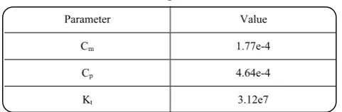
Table 1: Kinetic parameters [19].

Parameter Value

Cm 1.77e-4

Cp 4.64e-4

Kt 3.12e7

the number of monomers and branching points in each chain. I, M and S are the initiator, monomer and solvent molecules. Kd, Kp, Ktrm, Ktrp, Ktrs, Kp*, Ktc, Ktdare the rate

constants of initiator decomposition, propagation, chain transfer to monomer, polymer and solvent, terminal double bond polymerization and termination by combination and disproportionation respectively.

The mass balances and moment equations for solution polymerization of vinyl acetate in a batch reactor, based on the kinetic scheme, are explained in appendix A. The kinetic parameters for mathematical modeling, which are reported in the literature, are listed in table 1. Some of the kinetic parameters of the model were not reported in the literature at the operating conditions used in this research, so these parameters are selected as decision variables to be optimized.

As discussed earlier, for parameter optimization of polymerization reaction, in the first step, mathematical modeling of free radical solution polymerization of vinyl acetate is carried out. Then by comparing experimental data with mathematical model and minimizing the objective functions, kinetic parameters which are transfer constant to methanol as solvent (Cs), initiator efficiency

(f) and terminal double bound reactivity (K) were determine in this study.

The objective function, I*, is a vector and consists of minimization of two error functions (objectives). To define the feasible domains of reaction temperature and conversion, two constraints are added to the problem. The objective functions and problem constraints are defined as follow:

(

)

* * *

1 2

I ≡ I , I (21)

n _nExp

* 1

i 1 _{nModel i} M

I Min 1

M =

≡ ∑ − (22)

n _Exp

* 2

i 1 _{Model i} I

I Min 1

I =

≡ ∑ − (23)

Table 2: Genetic algorithm parameters.

Population size ₄₀

Cross over probability 75%

Mutation probability 3.33%

subject to:

reaction 1

T=T ±Tol (24)

final reaction 2

x =x ±Tol (25)

Minimizing the objective (error) functions implies the obtaining optimized kinetic parameters near the global values in the reasonable computational cost.

EXPERIMENTAL

Polyvinyl acetate was produced from solution polymerization of vinyl acetate (VAc). Because chain transfer to methanol is low and the byproduct (methyl acetate) can be separated easily, methanol (MeOH) was selected as solvent. Azobisisobutironitrile (AIBN) was used as initiator because of lower chain transfer constant and production possibility of polyvinyl acetate with high molecular weight. At first, distilled vinyl acetate and methanol were introduced to a small glass reactor with agitator (400 rpm). The mixture was then heated to 59 °C, which is the reflux temperature and best for AIBN decomposition, and initiator was added. When poly-merization was completed, the system was cooled and finally produced polymer was washed, precipitated by water, dried at 45 °C in an oven and weighted.

The FTIR peaks of the produced polyvinyl acetate were in good agreement with the standard curve. Moreover, the GPC tests were done for molecular weight determination of produced polyvinyl acetate with polystyrene calibration between 34000-330000.

The effects of operating variables such as polymerization time, monomer to solvent ratio and initial concentration of initiator as shown in the following Figs. are considered.

RESULTS AND DISCUSSION

By the method discussed above, optimum values of kinetic parameters are obtained.

Table 3: Optimized kinetic parameters.

Parameter Optimized value

Cs 1.19e-3

K 0.46

f 0.9

The optimized values of objective kinetic parameters, obtained by comparing mathematical modeling results with experimental data and minimizing error functions described earlier, are listed in table 3.

The validity of genetic algorithm optimization technique used in this study is justified by comparing the results of mathematical modeling by optimized parameters with experimental data as shown in Figs. 4-7. Experimental and modeling results of final conversion versus initial concentration of initiator are shown in Fig. 4. By increasing the initial concentration of initiator, the conversion is increased but due to higher radical concentration, molecular weight is reduced.

Fig. 5 shows the experimental and modeling results of conversion versus reaction time. By increasing time and propagation of the reaction, the conversion is increased but the branching is also increased. Therefore at an optimum conversion, about 70%, the branching is low and also the cost of monomer recovery in the industrial plant is acceptable.

Experimental and modeling results of weight average molecular weight of polymer versus initial ratio of monomer to solvent are shown in Fig. 6. As the following Fig shows, by increasing the monomer to the solvent volume ratio the solvent radical decreases and the molecular weight of polyvinyl acetate increases. The monomer to solvent ratio of 3/1 is chosen for high molecular weight and also acceptable viscosity of mixing of the solution.

Experimental and modeling results of molecular weight distribution of produced polymer at x = 68% obtained by optimized parameters, are presented in Fig. 7.

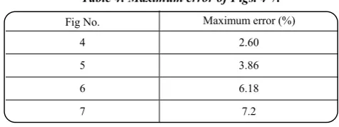
The maximum error in Figs. 4-7, calculated from equation (26), to predict product properties by application of optimized parameters are summarized in table 4.

⎟⎟ ⎟ ⎠ ⎞ ⎜⎜

⎜ ⎝

⎛ ₋

= *100

y y y Max Error Max

exp , i

el mod , i exp , i

(26)

Table 4: Maximum error of Figs. 4-7.

Fig No. Maximum error (%)

4 2.60

5 3.86

6 6.18

7 7.2

The Pareto optimal set of objective functions and the decision variables set, which are terminal double bond reactivity and transfer constant to solvent in this study, obtained in the multi-objective optimization of the polymerization process are shown in Figs. 8 and 9 respectively.

CONCLUSIONS

Genetic algorithm has been used to optimize kinetic parameters of vinyl acetate polymerization in the presence of methanol as solvent. For this purpose at first, mathematical modeling of polymerization reaction based on the discussed model is done and then by minimizing the error functions define as differences between mathematical results and experimental data, the kinetic parameters are optimized.

The important properties of polymeric product, obtained by mathematical modeling of polymerization process using optimized kinetic parameters, are in good agreement with the experimental data as shown in Figs. 4-7.

It is found that by genetic algorithm technique, objective parameters are determined near the global optimum without requiring much more information about the system, in contrast to the traditional techniques, which need gradients or initial guesses.

Nomenclatures

Bn Number average branching density

Bw Weight average branching density

Cm Transfer constant to monomer defined as: Ktrm/Kp

Cp Transfer constant to polymer defined as: Ktrp/Kp

Cs Transfer constant to solvent defined as: Ktrs/Kp

f Initiator efficiency I Initiator molecule I* Objective function K Terminal double bound reactivity defined as: Kp*/Kp

Fig. 4: Effect of initial concentration of initiator on the final conversion.

Fig. 5: Comparison between simulated and experimental conversion versus time.

Fig. 6: Effect of initial ratio of monomer to solvent on weight average molecular weight of polymer.

Fig. 7: Comparison between simulated and experimental molecular weight distribution of poly vinyl acetate obtained at x = 68%.

Fig. 8: Pareto optimal set of objective functions.

Fig. 9: Decision variable set for the optimization of vinyl acetate polymerization process.

0.00E+00 2.00E+05 4.00E+05 6.00E+05 8.00E+05

Molecular Weight 1.25

1

0.75

0.5

0.25

0

MWD

Model Experimental

0.00E+00 2.50E-03 5.00E-03 7.50E-03 1.00E-02 1.25E-02

Initial Concentration of Initiator, mol/lit 80

70

60

50

40

Co

n

v

ersi

o

n

Model Experimental

0 0.1 0.2 0.3

F2 0.5

0.4

0.3

0.2

0.1

0

F1

0.45 0.455 0.46 0.465 0.47

Terminal double bond reactivity 0.0012

0.00119

0.0018

0.00117

Tra

n

sfer

co

n

sta

n

t

to

sol

v

en

t

0 1 2 3 4

Time, hr 80

70

60

50

40

Co

n

v

ersi

o

n

Model Experimental

200000

150000

100000

50000

0

Mw

0 1 2 3 4

VAc/MeOH Model

Kp Rate constant of propagation

Kp* Rate constant of terminal double bond

polymerization Kt Rate constant of termination

Ktc Rate constant of termination by combination

Ktd Rate constant of termination by

disproportionation Ktrm Rate constant of chain transfer to monomer

Ktrp Rate constant of chain transfer to polymer

Ktrs Rate constant of chain transfer to solvent

M Monomer molecule Mn Number average molecular weight

Mw Weight average molecular weight

m0 Monomer molecular weight

Pr,b Polymer molecule consists of r monomers and

b branching points without terminal double bond P'r,b Polymer molecule consists of r monomers and

b branching points with terminal double bond Pºr,b Radical chain consists of r monomers and b branching points without terminal double bond Pº'r,b Radical chain consists of r monomers and b branching points with terminal double bond

Rº Primary free radical

S Solvent molecule

T Temperature

Tol1, Tol2 Tolerance

x Conversion

APPENDIX A

Equations of Mathematical Modeling

Polymerization of vinyl acetate is mathematically modeled on the basis of published works [20,21]. Equations of mathematical modeling of vinyl acetate polymerization are obtained by writing mass balance for each species. These equations describe the behaviour of the system as a function of conversion as below [20]:

x 1 KQ C dx dQ 0 m 0 − −

= (A-1)

x 1 ] S [ C dx Q

d 0 s

− = ′ (A-2) − − + = Z ) x 1 ( C Q C dx

dQ1 p 1 m _(A-3)

{

}

) x 1 ( Z Q C ] S [ C

KQ_{1 s p 1}

− ′ + ⎭ ⎬ ⎫ ⎩ ⎨ ⎧ + ′ ⎭ ⎬ ⎫ ⎩ ⎨ ⎧ − + = ′ Z Q C ] S [ C x 1 KQ 1 dx Q

d 1 1 s p 1 _(A-4)

(

+ ′

)

₌ = dx Q Q d dx

dQT2 2 2 _(A-5)

(

)

(

)

⎥ ⎥ ⎦ ⎤ ⎢ ⎢ ⎣ ⎡ − + − + + − Z Q C KQ x 1 KQ x 1 x 1

2 1 1 p T2

(

)

1 dx Q Q d dx

dQ1T ₌ 1+ 1′ ₌

(A-6) + − − = x 1 KH Q C dx

dH0 p 1 0 _(A-7)

(

)

⎭ ⎬ ⎫ ⎩ ⎨ ⎧ − + − + x 1 Q C ) x 1 ( C Z Q H

K 0 0 m p 1

(

)

Z * Q H K x 1 Q C dx H

d 0 p 1 ₊ 0+ 0

− ′ = ′ (A-8) ⎭ ⎬ ⎫ ⎩ ⎨ ⎧ − ′ + x 1 Q C ] S [

Cs p 1

=

dx dH1T

(A-9)

(

)

(

)

{

+ + +

}

+ ⎥ ⎦ ⎤ ⎢ ⎣ ⎡ − + − 0 0 T 1 p 1 Q H K x H C ) x 1 ( Z KQ x 1

(

)

_[

_]

1 T 2 p 0 0 1 T 2 p KQ x 1 Q C ) x 1 ( Z Q H K x 1 KQ Q C + − + − + + ⎥ ⎥ ⎦ ⎤ ⎢ ⎢ ⎣ ⎡ − +

used parameters in the above equations are defined as:

p * p p trl 1 K K K , s , p , m 1 , K K

C = = = (A-10)

] S [ C x C ) x 1 ( C

Z= _m − + _p + _s (A-11)

(

)

_∑∑

∞

(

)

= ∞ = ′ + = ′ + = 1 r b 0

b , r b , r 0 0 T

0 Q Q P P

Q (A-12)

(

)

(

)

0 n T 0 1

r b 0

b , r b , r 1 1 T 1 m M Q P P r Q Q

Q = + ′ =

∑∑

⋅ + ′ =

∞ = ∞ = (A-13)

(

+ ′

)

= ⋅

(

+ ′

)

= =

∑∑

∞ = ∞ = 1 r b 0

b , r b , r 2 2 2 T

2 Q Q r P P

Q (A-14)

∑∑

∞

= ∞ =

=

1 r b 0

b , r 0 bP

H (A-15)

∑∑

∞

= ∞ =

′ =

′

1 r b 0

b , r 0 bP

H (A-16)

Bn Q H H

HT0 = 0 + 0′ = T0 (A-17)

(

P P

)

H H xBw

rb

H _{1 1}

1 r b 0

b , r b , r T

1 =

∑∑

+ ′ = + ′ =

∞ =

∞ =

(A-18)

td tc t K K

K = + (A-19)

where m0 is the molecular weight of monomer and Mn

and Mw are the number and weight average molecular

weight of polymer.

Temperature relation of some kinetic parameters used in this study is introduced in the following equations [22]:

) RT / 34000 exp( * 16 e 9 . 7

Kd = − (A-20)

) RT / 4200 exp( * e 13 . 1

Kp = − (A-21)

Received : 19th July 2006 ; Accepted : 20thNovember 2006

REFERENCES

[1] Holland, H.J., Adaptation in Natural and Artificial Systems, An Introductory Analysis with Application to Biology, Control and Artificial Intelligence, The university of Michigan Press, Ann Arbor, USA (1975).

[2] Bhaskar, V., Gupta, S.K., Ray, A.K.,Comput. Chem. Eng.25, 391 (2001).

[3] Silva, C.M., Biscaia Jr, E.C., Comput. Chem. Eng., 27, 1329 (2003).

[4] Rantow, F.S., Soroush, M., Grady, M.C., American Control Conference (ACC), Portland, Oregon, June 8-10, 3102 (2005)

[5] Massebeuf, S., Fonteix, C., Hoppe, S., Pla, F., J. Appl. Polym. Sci.,87, 2383 (2003).

[6] Zhou, F., Gupta, S.K., Ray, A.K., J. Appl. Polym. Sci.,78, 1439 (2000).

[7] Mitra, K., Majumdar, S., Raha, S., Comput. Chem. Eng.,28, 2583 (2004).

[8] Mitra, K., Deb, K., Gupta, S.K.,J. Appl. Polym. Sci., 69, 69 (1998).

[9] Garg, S., Gupta, S.K., Macromol. Theory Simul., 8, 46 (1999).

[10] Mitra, K., Majumdar, S., Raha, S., Ind. Eng. Chem. Res.,43, 6055 (2004).

[11] Sarkar, D., Modak, J.M., Chem. Eng. Sci.,58, 2283 (2003).

[12] Sarkar, D., Modak, J.M., Comput. Chem. Eng., 28, 789 (2004).

[13] Sarker, D., Modak, J.M., Chem.Eng. Sci., 60, 481 (2005).

[14] Goldberg, D. E., Genetic Algorithms in Search Optimization and Machine Learning, Addison-Wesley (1989).

[15] Renner, G., Ekart, A., Comput. Aid. Des.,35, 709 (2003).

[16] Marseguerra, M., Zio, E., Podofillini, L., Ann. Nucl. Energy.,30, 1437 (2003).

[17] Wang, Y.Z., Expert Systems with Applications,25, 39 (2003).

[18] Pareto, V., “Manuale di economica politica, Societa Editrice Libraria”, Milan (1906), Translated into English by A.S. Schwier as Manual of Political Economy, Ed. Schwier, A. S. and Page, A.N., Kelly, A.M., New York (1979).

[19] Polymer Handbook (Eds: Brandrup J. and Immergut E.H.), John Wiley & Sons, New York (1975). [20] Graessley, W.W., Hartung, R.D., Uy W.C., J. Polym.

Sci. Part A-2.,7, 1919 (1969).

[21] Villermaux, J., Blavier, L., Chem. Eng. Sci.,39, 87 (1984)