44
COVARIATES AND SAMPLE SIZE EFFECTS ON PARAMETER ESTIMATION FOR BINARY LOGISTIC REGRESSION MODEL
Hamzah Abdul Hamid1, Yap Bee Wah2, Xian-Jin Xie3
1,2Faculty of Computer and Mathematical Sciences, Universiti Teknologi MARA, 40450 Shah Alam, Selangor Malaysia
3Department of Clinical Sciences & Simmons Cancer Center, The University of Texas Southwestern Medical Center, 5323 Harry Hines Blvd. Dallas, Texas, USA
1Institute of Engineering Mathematics, Universiti Malaysia Perlis, Kampus Pauh Putra, 02600 Arau, Perlis *Corresponding Author: [email protected]
ASTRACT The types of covariate and sample size may influence many statistical methods. This study involves a rigorous Monte Carlo simulation to illustrate the effect of different types of covariate and sample size on parameter estimation for binary logistic regression model. The simulation study covers different sample sizes and types of covariate (continuous, count, categorical). This study shows how the MLE parameter estimates are affected by different types of covariate. The simulation results confirm that the parameter estimates improves as sample size increases. Results for single normal, two normal, categorical and count covariateshow that sample size below 50 produced highly biased estimates. For model with skewed covariate, sample size of 150 and below produced biased estimates. The variability of parameter estimate increases when of the Poisson distribution increases. An application to a real data set confirms the results of the simulation study.
ABSTRAK Jenis pembolehubah tidak bersandar dan saiz sampel boleh mempengaruhi pelbagai kaedah berstatistik. Kajian ini mengkaji secara teliti menggunakan simulasi Monte Carlo dan seterusnya memperlihatkan kesan perbezaan pembolehubah tidak bersandar dan saiz sampel terhadap penganggaran parameter bagi model regresi logistik binari. Kajian simulasi dengan perbezaan saiz sampel dan jenis pembolehubah tidak bersandar (selanjar, kiraan, berkategori) telah dijalankan. Kajian ini menunjukkan bagaimana penganggaran kemungkinan maksima dipengaruhi oleh jenis pembolehubah tidak bersandar. Kajian simulasi menunjukkan penganggaran parameter semakin baik sejajar dengan peningkatan saiz sampel. Keputusan bagi model yang mempunyai satu dan dua pembolehubah tidak bersandar normal, satu pembolehubah berkategori dan kiraan menunjukkan saiz sampel kurang dari 50 menghasilkan penganggaran parameter yang sangat tidak tepat. Bagi model dengan pembolehubah tidak bersandar yang bertaburan tidak normal, saiz sampel 150 dan kurang menghasilkan penganggaran parameter yang tidak tepat. Variasi anggaran parameter meningkat apabila bagi taburan Poisson meningkat. Suatu aplikasi terhadap data sebenar mengesahkan dapatan kajian simulasi.
(Keywords: Parameter estimation, simulation, binary logistic regression, MLE)
INTRODUCTION
Regression methods have become an integral component in exploring the relationship between a response variable and one or more explanatory variables. The difference between linear regression model
45 categorical independent variable (Kutner M. H. et al, 2004; Hosmer Jr. D. & Lemeshow S., 2004). Logistic regression model is a very important statistical model and is widely used in medical (Bender R. & Grouven U., 1997; Siqueira A. L. & Cardoso C. S., 2008; Citko D. et al, 2012) epidemiology (Ancel P. Y., 1999; Burguet A., 2004; Astolfi P. et al, 2006), psychology (Rosenfeld B. & Penrod S. D.,2011; Eke G. at al, 2012), business (Puagwatana S. & Gunawardana K. D., 2005; Hauser R. P. & Booth D., 2011), finance (Bensic M. et al, 2005; Han D. et al, 2008) and social (Howell-M N. & Proctor E., 1993; Fullerton A. S., 2009) research.
One of the major applications of statistical modeling is estimating the population parameters from sample statistics. In regression modeling, there are two general methods of parameter estimation which are least-squares estimation (LSE) and maximum likelihood estimation (MLE). MLE has several optimal properties such as sufficiency, consistency, efficiency and parameterization invariance (Myung I., 2003). In fitting a logistic regression model, the MLE is used to estimate the model parameters. This method is suitable to be applied to problems associated with binary response variable. In the MLE method, the likelihood function must first be constructed. Then, the Newton Raphson Iterative method is used to obtain the value ofˆ. Newton-Raphson is an efficient method based on the idea of linear approximation.
The distribution of covariates may affect the statistical parametric methods. The use of classical parametric methods such as Student’s t, Analysis of Variance (ANOVA) and ordinary least squares regression when the assumption (e.g., normality) is violated, can lead to the inaccurate calculation of p
value and confidence interval (Hurn E. D.
M. & Mirosevich V. M., 2008). The simulation study by (Jahan S. & Khan A ,2012) shows that the power of t-test for the simple linear regression model was affected by sample size, skewness and kurtosis. The performance of the t-test was determined by calculating Type I error while the power of the t-test was evaluated by calculating the probability that Type II error will not occur. (Khan A. & Rayner G., 2003) investigated the effect of deviating from the normal distribution assumption for ANOVA and Kruskal-Wallis test. The results showed that both tests are affected by the kurtosis of the error distribution, but less affected by the skewness. (Curran P. J. et al, 1996) reported that the violation of the assumption of normality affects the normal theory maximum likelihood 2 test in confirmatory factor analysis. Additionally, the Browne’s asymptotic distribution free
2
is affected by normal and non-normal data for small sample size, but is unbiased at sample sizes of 500 and above regardless of distribution, while the Satorra-Bentler rescaled 2 showed that non-normal data stop affecting this test at sample size of 200 and above. (Whittemore A.,1981) found that sample size in modeling logistic regression is affected by distributions of covariate (Normal, Exponential, Poisson, Bernoulli).
46 1996) to deal with multicollinearity for the linear regression problem was extended by (Kim Y. & Kim J., 2006) for logistic regression. However, they used independent covariates in their study. Thus, future research may consider the performance of logistic regression if multicollinearity of the covariates exists and the most effective way to deal with this problem.
In a logistic regression model, several methods have been proposed to calculate sample size (Whittemore A.,1981), (Self, S. & Mauritsen, R., 1988; Hsieh F. Y.,1989; Hsieh F. Y. et al,1998; Demidenko E., 2006). Most of the methods did not illustrate the effect of the count covariate in the model. The effect of different distributions also has not been investigated rigorously. (Hamid H.A. et al., 2015), investigated the effect of different sample size and distribution of a continuous covariate on
parameter estimation. The distributions were limited to; N(0,1), Beta(4,2) and U(-3, 3). This study extends (Hamid H.A. et al.,2015) simulation study by considering positively and negatively skewed continuous distribution, count and categorical covariate. The aim of this study is to assess rigorously the effects of different types of covariate (continuous, count, categorical) and distributions on the MLE parameter estimates for the binary logistic regression model via a Monte Carlo simulation study. The simulation was carried out using R an open-source programming software.
In Section 2, we present a brief review of the binary logistic regression model followed by the simulation procedure in Section 3. The simulation results are discussed in Section 4 and an application to a real dataset is shown in Section 5. Some discussions and conclusion are in Section 6.
BINARY LOGISTIC REGRESSION MODEL
Generalized Linear Models (GLMs) are an extension of the traditional linear modeland were introduced by (Nelder J. & Baker R., 1972). In GLMs, the response variable yi is
assumed to follow an exponential family distribution with mean i which is assumed
to be some function of xTi , where i is often a nonlinear function of the covariates. The GLMs are the broad class models that include lots of model such as linear regression, ANOVA, Poisson regression and log-linear model. Generally, there are three components to any GLMs, which are random component - refers to the probability distribution of the response variable Y; systematic component - specifies the explanatory variables X in the model; and link function, or g
- specifies the link between random and systematiccomponents. The linear combination of predictor variables is connected to the dependent variable via a link function. The link function such as logit, probit and log-linear connects the means of the response to the linear predictors and handles non-normality effectively. The GLM model can be expressed as:
'i
i g x
y
E where E
yi is the mean ofthe response, g is the link function and xi'
is the linear predictor. In binary logistic regression model, the logit link function is often being used.
Let n be the number of observations with binary outcomes denoted by Y which have value “0” and “1”. The event of interest is coded as “1” or “0” otherwise. Let the vectorx'(x1,x2,x3,...,xk)denote the set of k
47
event can be expressed by (Hosmer D. & Lemeshow S., 1980): thus,
( 1 )
0 1
0
1 |
1 i
x x
i e e x
x X Y P
hi k h
h k
h hi h
(1)
Y X xi
xiP 0| 1 (2)
The explanatory or predictor variable xi may be quantitative (continuous), qualitative (discrete) or both (mixed). This study considered single and two predictor variables only.
SIMULATION PROCEDURES
The simulations were performed using R an open source programming software. For each simulation, the sample size of 30, 50, 100, 150, 300, 500, 1000, 1500, 3000 and 5000 were considered. The data were generated using the technique used by (Xie X.-J. et al, 2008). For a given set of value for and n:
(1) Generate covariate x from the stated distribution
(2) Evaluate the binary logistic regression probabilities, 0 and 1
(3) Generate the data u from a uniform distribution, U(0,1)
(4) Generate outcomes for binary logistic regression by using the rule y=1 if
xu and y=0 otherwise
(5) Fit binary logistic regression model to the data.
(6) Repeat (1)-(5) for 10000 replications. (7) Calculate the mean of .
(8) Calculate the 95% Confidence Interval (CI) for .
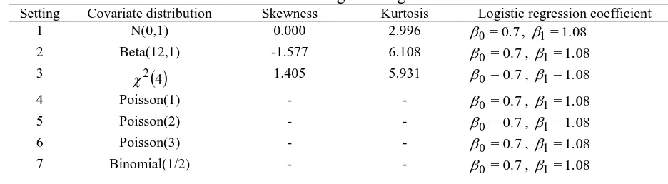
To obtain 95% confidence interval (CI) for , we first obtain parameter estimates for 10,000 replications. The 95% CI is the 2.5th percentile and 97.5th percentile of the parameter estimates from 10000 replications. The distributions of the covariate and the true parameters for binary logistic regression model are presented in Table 1. The N(0,1) distribution yields continuous data with symmetric distribution, while Beta (12,1) and 2
4 produced negatively skewed and positively skewed continuous distribution respectively. The Poisson (1), Poisson (2) and Poisson (3) were chosen to represent count data with different . The binary categorical data were generated by using Binomial (1/2) distribution. These distributions were selected to cover various types of data for a covariate. The simulation was carried out using 10,000 replications. The R codes for the simulation are given in Appendix 1.Table 1. Distributions of Covariate and True Logistic Regression Coefficient
Setting Covariate distribution Skewness Kurtosis Logistic regression coefficient
1 N(0,1) 0.000 2.996 0 =0.7, 1=1.08
2 Beta(12,1) -1.577 6.108 0 =0.7, 1 =1.08
3 2
4 1.405 5.931 0 =0.7, 1 =1.084 Poisson(1) - - 0 =0.7, 1 =1.08
5 Poisson(2) - - 0 =0.7, 1 =1.08
6 Poisson(3) - - 0 =0.7, 1 =1.08
48
8 N(0,1) and N(0,1) 0.000 and 0.000 2.996 and 2.996 0 =0.7, 1=1.08, 2 =1.69
9 N(0,1) and Beta(12,1) 0.000 and -1.577 2.996 and 6.108 0 =0.7, 1=1.08, 2 =1.69
10 N(0,1) and
4
2
0.000 and 1.405 2.996 and 5.931 0 =0.7, 1=1.08, 2 =1.69
SIMULATION RESULTS
This section presents the simulation results. We chose various distributions of data to represent various situations in practice. The aim is to cover three different types of data (one continuous, two continuous, count and categorical) and this yields seven distributions to be considered in the simulation procedures.
Continuous Data in Covariates
First, we considered three different continuous distributions to investigate the effect on the estimation of the parameter for a simple binary logistic regression. The distribution N(0,1) was chosen to represent normal data, Beta(12,1) represents negatively skewed data and2(4)
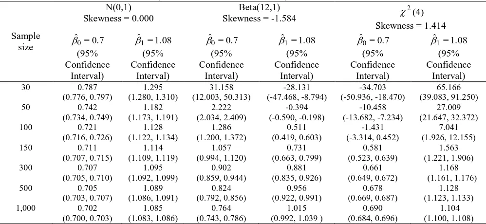
represents positively skewed data. Table 2 summarizes the results of the parameter
estimates for different distributions of covariate for different sample size. In addition, we provide the 95% confidence interval for parameter estimation at different level of sample size. Results show that small sample size (n=30) yields poor estimation of
0
and 1 for all types of distribution. The parameter estimates for skewed covariate are severely affected when the sample size is small. When covariates are normal or positively skewed, the estimated value for
1
were higher than the set value. On the other hand, when sample size is less than 300 and covariate are negatively skewed, the estimated parameter is less than the set value. The estimation of both parameters 0 and 1 for normal distributions gets closer to the true parameter values at sample size of 100 and above while negatively skewed and positively skewed distributions require at least 1500 and 500 respectively to be close to the true parameter value.
Table 2. Parameter Estimates (Model with One Covariate)
Sample size
N(0,1) Skewness = 0.000
Beta(12,1) Skewness = -1.584
2
(4) Skewness = 1.414 0.7 = ˆ 0 (95% Confidence Interval) 1.08 = ˆ 1 (95% Confidence Interval) 0.7 = ˆ 0 (95% Confidence Interval) 1.08 = ˆ 1 (95% Confidence Interval) 0.7 = ˆ 0 (95% Confidence Interval) 1.08 = ˆ 1 (95% Confidence Interval)
30 0.787
(0.776, 0.797) 1.295 (1.280, 1.310) 31.158 (12.003, 50.313) -28.131 (-47.468, -8.794) -34.703 (-50.936, -18.470) 65.166 (39.083, 91.250)
50 0.742
(0.734, 0.749) 1.182 (1.173, 1.191) 2.222 (2.034, 2.409) -0.394 (-0.590, -0.198) -10.458 (-13.682, -7.234) 27.009 (21.647, 32.372)
100 0.721
(0.716, 0.726) 1.128 (1.122, 1.134) 1.286 (1.200, 1.372) 0.511 (0.419, 0.603) -1.431 (-3.314, 0.452) 7.041 (1.926, 12.155)
150 0.711
(0.707, 0.715) 1.114 (1.109, 1.119) 1.057 (0.994, 1.120) 0.731 (0.663, 0.799) 0.581 (0.523, 0.639) 1.563 (1.221, 1.906)
300 0.707
(0.705, 0.710) 1.095 (1.092, 1.099) 0.902 (0.859, 0.944) 0.881 (0.835, 0.926) 0.661 (0.649, 0.672) 1.168 (1.161, 1.176)
500 0.705
(0.703, 0.707) 1.089 (1.086, 1.091) 0.824 (0.792, 0.856) 0.956 (0.922, 0.991) 0.678 (0.669, 0.687) 1.128 (1.123, 1.133)
1,000 0.702
(0.700, 0.703) 1.085 (1.083, 1.086) 0.764 (0.743, 0.786) 1.015 (0.992, 1.039 )
0.690 (0.684, 0.696)
49
1,500 0.701
(0.700, 0.702)
1.083 (1.081, 1.084)
0.714 (0.697, 0.732)
1.067 (1.048, 1.087)
0.694 (0.689, 0.699)
1.095 (1.092, 1.098)
3,000 0.701
(0.700, 0.702)
1.081 (1.080, 1.082)
0.714 (0.701, 0.726)
1.068 (1.054, 1.081)
0.696 (0.693, 0.700)
1.088 (1.086, 1.090)
5,000 0.701
(0.700, 0.702)
1.081 (1.080, 1.081)
0.699 (0.689, 0.708)
1.083 (1.072, 1.093)
0.701 (0.698, 0.703)
1.083 (1.081, 1.084)
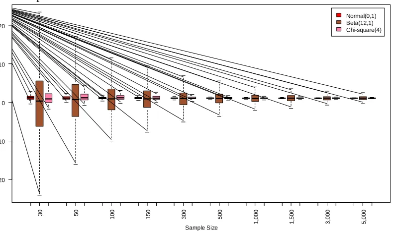
The box-plots for parameter estimates 1 for different sample sizes and different distributions of covariate are shown in Figure 1. The parameter estimate gets closer to the true value when the sample size increases. The box-plots shows that for all
covariate distributions the standard deviation decreases as sample size increases. The parameter estimate for negatively skewed covariate has largest variability compared to normal covariate or positively skewed covariate.
Figure 1. Box-plots of parameter estimates (ˆ1) for continuous covariate
Next we investigate the effects of different data distributions when the model contains more than one covariate. The data for the model that contains two continuous variables was generated. At least one of the covariate distributions in this model is from N(0,1). This is to avoid severe imbalanced data set being generated for the dependent variable. The results of this simulation study are summarized in Table 3. The results obtained are consistent with the results for a single covariate. The estimation for 0, 1 and 2 for a model that contains skewed covariate are severely affected at small
sample size. The model that contains no skewed covariate is less affected and the estimates approach true parameter values at sample size of 500. The model that contains skewed covariate need more than 500 to obtain reliable parameter estimates.
The box-plots for parameter estimates ˆ2 for different sample sizes and different distributions of covariate by excluding sample size of 30 are shown in Figure 2. Consistent with the results obtained for a single covariate model, the estimates approaches the true value when the sample size increases. The box-plots show that the
30 50
100 150 300 500
1
,0
0
0
1
,5
0
0
3
,0
0
0
5
,0
0
0
-20 -10 0 10 20
Sample Size
50 standard deviation for all covariate distributions decreases as sample size increases. The parameter estimate for the model that contains one skewed covariate has largest variability compared to the model that contains both normal covariate.
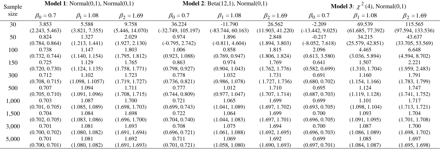
The Mean Squared Error (MSE) measures how close the fitted ˆ is to the true value
.Table 4 shows the Mean Squared Error (MSE) for all three models. The MSE is very large when n is small and for skewed covariate.
Figure 2. Box-plots of parameter estimates (ˆ2)
Model 1 : Two N(0,1) covariates;
Model 2 : One N(0,1) and one Beta(12,1) covariates; Model 3 : One N(0,1) and one 2(4) covariates.
Table 4. Mean Squared Error (Model with Two Covariates)
Sample size
Model 1: Normal(0,1), Normal(0,1)
Model 2: Beta(12,1), Normal(0,1)
Model 3:
2
(4), Normal(0,1) 0.7
=
0
1=1.08 2=1.69 0=0.7 1=1.08 2=1.69 0=0.7 1=1.08 2=1.69
30 6752.094 8146.231 48450.34 12381058 13472894 559792.3 328394 165191.5 853380.7
50 4.144 33.922 27.074 8137.587 19081.91 2371.764 159748.8 195187.7 258465.7
100 0.095 0.133 0.203 17.724 20.504 0.236 5726.809 5327.336 11004.47
150 0.058 0.080 0.117 10.786 12.513 0.132 8.896 101.375 178.713
300 0.027 0.036 0.052 4.719 5.500 0.060 0.311 0.096 0.175
500 0.016 0.021 0.029 2.743 3.191 0.034 0.173 0.048 0.092
1,000 0.008 0.010 0.014 1.286 1.504 0.016 0.084 0.022 0.041
1,500 0.005 0.007 0.010 0.858 1.005 0.011 0.055 0.014 0.027
3,000 0.002 0.003 0.005 0.428 0.500 0.005 0.026 0.007 0.013
5,000 0.002 0.002 0.003 0.264 0.310 0.003 0.016 0.004 0.008
50 100 150 300 500
1,
00
0
1,
50
0
3,
00
0
5,
00
0
-2 0 2 4 6 8
Sample Size
51 Table 3. Parameter Estimates (Model with Two Covariates)
Sample size
Model 1: Normal(0,1), Normal(0,1) Model 2: Beta(12,1), Normal(0,1) Model 3: 2(4), Normal(0,1)
0.7 =
0
1=1.08 2=1.69 0=0.7 1=1.08 2=1.69 0=0.7 1=1.08 2=1.69
30 3.853
(2.243, 5.463) 5.588 (3.821,7.355) 9.758 (5.446, 14.070) 36.224 (-32.749, 105.197) -11.790 (-83.744, 60.163) 26.562 (11.903, 41.220) -2.209 (-13.442, 9.025) 69.539 (61.685, 77.392) 115.565 (97.594, 133.536)
50 0.824
(0.784, 0.864) 1.327 (1.213, 1.441) 2.029 (1.927, 2.130) 0.974 (-0.795, 2.742) 1.896 (-0.811, 4.604) 2.848 (1.894, 3.803) -0.217 (-8.052, 7.618) 34.215 (25.579, 42.851) 43.637 (33.705, 53.569)
100 0.738
(0.732, 0.744) 1.147 (1.140, 1.154) 1.803 (1.795, 1.812) 1.006 (0.923, 1.088) 0.858 (0.769, 0.947) 1.815 (1.806, 1.824) 2.096 (0.613, 3.580) 4.465 (3.036, 5.894) 6.648 (4.594, 8.702)
150 0.725
(0.720, 0.730) 1.129 (1.124, 1.135) 1.765 (1.758, 1.771) 0.863 (0.798, 0.927) 0.974 (0.904, 1.043) 1.769 (1.762, 1.776) 0.641 (0.582, 0.699) 1.507 (1.310, 1.704) 2.221 (1.959, 2.483)
300 0.712
(0.708, 0.715) 1.102 (1.098, 1.1057) 1.723 (1.719, 1.727) 0.778 (0.736, 0.821) 1.032 (0.986, 1.078) 1.731 ( 1.727, 1.736)
0.691 (0.680, 0.702) 1.160 (1.154, 1.166) 1.791 (1.783, 1.799)
500 0.707
(0.705, 0.710) 1.094 (1.091, 1.096) 1.711 (1.708, 1.715) 0.777 (0.744, 0.809) 1.012 (0.977, 1.047) 1.710 (1.707, 1.714) 0.695 (0.687, 0.703) 1.124 (1.119, 1.128) 1.747 (1.741, 1.752)
1,000 0.703 (0.701, 0.705) 1.087 (1.085, 1.089) 1.700 (1.698, 1.703) 0.721 (0.699, 0.743) 1.065 (1.041, 1.089) 1.699 (1.697, 1.702) 0.699 (0.693, 0.705) 1.101 (1.098, 1.104) 1.717 (1.713, 1.721)
1,500 0.704 (0.702, 0.705) 1.084 (1.083, 1.086) 1.698 (1.696, 1.700) 0.722 (0.704, 0.740) 1.064 (1.044, 1.083) 1.699 (1.697, 1.701) 0.700 (0.696, 0.705) 1.093 (1.091, 1.095) 1.704 (1.701, 1.708)
3,000 0.701 (0.700, 0.702) 1.081 (1.080, 1.082) 1.693 (1.691, 1.694) 0.708 (0.696, 0.721) 1.075 (1.061, 1.088) 1.694 (1.692, 1.695) 0.700 (0.696, 0.703) 1.087 (1.086, 1.089) 1.700 (1.698, 1.702)
5,000 0.701
52
Count Data in Covariates
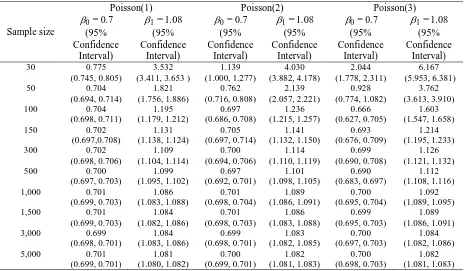
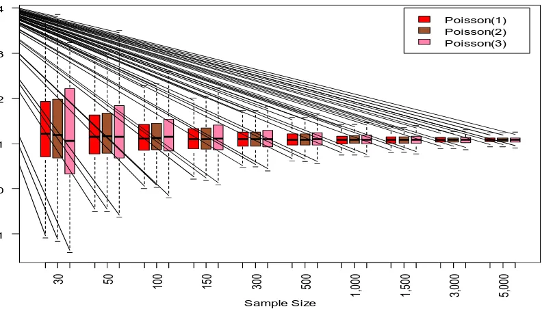
We used three different values of to generate Poisson distribution data. The values of 1, 2 and 3 were selected to represent the various situations in covariate. The simulation results are summarized in Table 5. As expected, small sample size (n=30) led to poor estimates of the model parameter, 0 and 1. The parameter estimate ˆ1 for all three distributions is higher than the set value
1 1.08
.The parameterestimates ˆ0 and ˆ1 were more severely affected for distribution with larger values of . The parameter estimates for Poisson (1) and Poisson (2) get closer to true parameter values at sample size of 1000 and above while the estimates for Poisson (3) the estimates only get closer to the true parameter value at sample size of 1500 and above.
Table 5. Parameter Estimates for Poisson Covariate
Sample size
Poisson(1) Poisson(2) Poisson(3)
0.7 = 0 (95% Confidence Interval) 1.08 = 1 (95% Confidence Interval) 0.7 = 0 (95% Confidence Interval) 1.08 = 1 (95% Confidence Interval) 0.7 = 0 (95% Confidence Interval) 1.08 = 1 (95% Confidence Interval)
30 0.775
(0.745,0.805)
3.532 (3.411,3.653 )
1.139 (1.000, 1.277) 4.030 (3.882, 4.178) 2.044 (1.778, 2.311) 6.167 (5.953, 6.381)
50 0.704
(0.694,0.714) 1.821 (1.756, 1.886) 0.762 (0.716, 0.808) 2.139 (2.057, 2.221) 0.928 (0.774, 1.082) 3.762 (3.613, 3.910)
100 0.704
(0.698, 0.711) 1.195 (1.179, 1.212) 0.697 (0.686, 0.708) 1.236 (1.215, 1.257) 0.666 (0.627, 0.705) 1.603 (1.547, 1.658)
150 0.702
(0.697,0.708) 1.131 (1.138, 1.124) 0.705 (0.697, 0.714) 1.141 (1.132, 1.150) 0.693 (0.676, 0.709) 1.214 (1.195, 1.233)
300 0.702
(0.698, 0.706) 1.109 (1.104, 1.114) 0.700 (0.694, 0.706) 1.114 (1.110, 1.119) 0.699 (0.690, 0.708) 1.126 (1.121, 1.132)
500 0.700
(0.697, 0.703) 1.099 (1.095, 1.102) 0.697 (0.692, 0.701) 1.101 (1.098, 1.105) 0.690 (0.683, 0.697) 1.112 (1.108, 1.116)
1,000 0.701
(0.699, 0.703) 1.086 (1.083, 1.088) 0.701 (0.698, 0.704) 1.089 (1.086, 1.091) 0.700 (0.695, 0.704) 1.092 (1.089, 1.095)
1,500 0.701
(0.699, 0.703) 1.084 (1.082, 1.086) 0.701 (0.698, 0.703) 1.086 (1.083, 1.088) 0.699 (0.695, 0.703) 1.089 (1.086, 1.091)
3,000 0.699
(0.698, 0.701) 1.084 (1.083, 1.086) 0.699 (0.698, 0.701) 1.083 (1.082, 1.085) 0.700 (0.697, 0.703) 1.084 (1.082, 1.086)
5,000 0.701
(0.699, 0.701) 1.081 (1.080, 1.082) 0.700 (0.699, 0.701) 1.082 (1.081, 1.083) 0.700 (0.698, 0.703) 1.082 (1.081, 1.083)
Figure 3 shows the box-plots of the parameter estimates for different sample sizes and different . Similarly, the parameter estimates approaches the true value when the sample size increases. The dispersion (standard deviation) of parameter
53 Figure 3. Box-plots of ˆ1 for Poisson Covariate
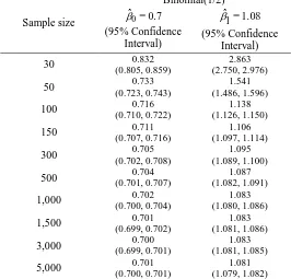
Categorical Data in Covariates
Then, the binomial distribution was generated to investigate the effects of a categorical covariate on parameter estimation for binary logistic regression. The distribution of Binomial(1/2) was used to generate data for binary covariate. Table 6 summarizes the results of parameter estimates for a binary covariate. The estimation is poor when sample size is small (n=30) as the estimated value for 1 are higher than the set value(1 1.08). The
parameter estimates, ˆ0 andˆ1 get closer to true parameter values at sample size 500.
Figure 4 shows the box-plots of the parameter estimates for a model with categorical covariate. It is shown that the sample size plays an important role in order to decrease inaccurate estimation of model parameters. The results for categorical covariate is consistent with the results obtained for continuous and count covariate. The dispersion (standard deviation) for both
0 ˆ
and
1 ˆ
decreases as sample size
increases.
30 50 100 150 300 500
1,
00
0
1,
50
0
3,
00
0
5,
00
0
-1 0 1 2 3 4
Sample Size
54
Table 6. Coefficient Parameter Estimates for Categorical Covariate
Sample size
Binomial(1/2) 0.7
= ˆ
0
(95% Confidence Interval)
1.08 = 1 ˆ
(95% Confidence Interval)
30 0.832
(0.805, 0.859)
2.863 (2.750, 2.976)
50 0.733
(0.723, 0.743)
1.541 (1.486, 1.596)
100 0.716
(0.710, 0.722)
1.138 (1.126, 1.150)
150 0.711
(0.707, 0.716)
1.106 (1.097, 1.114)
300 0.705
(0.702, 0.708)
1.095 (1.089, 1.100)
500 0.704
(0.701, 0.707)
1.087 (1.082, 1.091)
1,000 0.702
(0.700, 0.704)
1.083 (1.080, 1.086)
1,500 0.701
(0.699, 0.702)
1.083 (1.081, 1.086)
3,000 0.700
(0.699, 0.701)
1.083 (1.081, 1.085)
5,000 0.701
(0.700, 0.701)
1.081 (1.079, 1.082)
Figure 4. Box-plots of parameter estimation
ˆ1 for categorical covariateAN APPLICATION ON REAL DATA SET
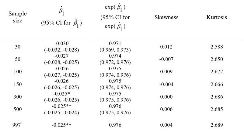
This section shows the parameter estimates by fitting a binary logistic regression model using the Intraoperative Hypothermia for Aneurysm Surgery Trial (Xie X.-J. et al, 2008; Todd M. M. et al, 2005) clinical data
set. The dependent variable is the Glasgow outcome score (GOS) (GOS=1 is favorable outcome and GOS=0 otherwise) which is used to measure whether mild intraoperative hypothermia improves long term neurologic outcome. The independent variables are hypothermia treatment (Yes=1, No=0), age in years, and the time in days from
30 50 100 150 300 500
1000 1500 3000 5000
55 subarachnoid hemorrhage (SAH) to induction. The sample size is 997 with 64.4% are Y=1. We repeatedly selected 1000 samples for each sample size of 30, 50, 100, 150, 300, 500 using stratified sampling. The
1 ˆ
and the 95% CI for the odds-ratio
are shown in Tables 7-9. Results show that the parameter estimate is affected by sample size. For the simple binary logistic model, only Age is a significant predictor of Glasgow outcome score (GOS).
Table 7. Parameter Estimates for hypothermia treatment (Categorical Variable)
Sample size
1 ˆ
(95% CI for 1 ˆ
)
Odds-ratio exp(
1 ˆ
) (95% CI for
exp( 1 ˆ
)
30 0.172
(0.122, 0.222)
1.659 (1.555, 1.764)
50 0.156
(0.118, 0.193)
1.402 (1.344, 1.459)
100 0.161
(0.136, 0.186)
1.275 (1.240, 1.309)
150 0.128
(0.108, 0.148)
1.197 (1.173, 1.222)
300 0.147
(0.134, 0.159)
1.181 (1.167, 1.196)
500 0.148
(0.140, 0.156)
1.169 (1.160, 1.179)
997+ 0.146 1.157
+Full orginal sample, *p<0.10, **p<0.05
Table 8. Parameter Estimates and Odds-Ratio for Age
Sample size
1 ˆ
(95% CI for 1 ˆ
)
exp( 1 ˆ
) (95% CI for
exp( 1 ˆ
)
Skewness Kurtosis
30 -0.030
(-0.032, -0.028)
0.971
(0.969, 0.973) 0.012 2.588
50 -0.027
(-0.028, -0.025)
0.974
(0.972, 0.976) -0.007 2.650
100 -0.026
(-0.027, -0.025)
0.975
(0.974, 0.976) 0.009 2.672
150 -0.026
(-0.026, -0.025)
0.975
(0.974, 0.976) -0.004 2.666
300 -0.025*
(-0.026, -0.025)
0.975
(0.975, 0.976) 0.000 2.686
500 -0.025**
(-0.025, -0.024)
0.976
(0.975, 0.976) 0.006 2.685
997+
-0.025** 0.976 0.004 2.689
+
56
Table 9. Parameter Estimates and Odds-Ratio for time in days from SAH to induction
Sample size
1 ˆ
(95% CI for 1 ˆ ) exp( 1 ˆ ) (95% CI for
exp( 1 ˆ
)
Skewness Kurtosis
30 -0.020
(-0.030, -0.009)
0.995
(0.984, 1.005) 1.504 4.984
50 -0.011
(-0.018, -0.004)
0.995
(0.988, 1.002) 1.555 5.155
100 -0.007
(-0.012, -0.003)
0.995
(0.991, 1.000) 1.612 5.313
150 -0.011
(-0.014, -0.007)
0.991
(0.987, 0.994) 1.618 5.343
300 -0.013
(-0.015, -0.011)
0.988
(0.986, 0.990) 1.625 5.340
500 -0.011
(-0.012, -0.009)
0.990
(0.988, 0.991) 1.638 5.381
997+ -0.011 0.989 1.637 5.367
+Full orginal sample, *p<0.10, **p<0.05
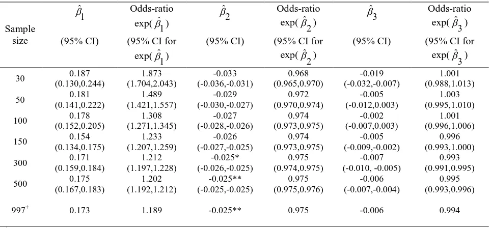
Table 10 summarized the results for a binary logistic regression model with three covariates which are hypothermia treatment (X1), age in years (X2) and the time in days from subarachnoid hemorrhage (SAH) to
induction (X3). The results were consistent with the single covariate model whereby only Age was significant for sample size 300 and above.
Table 10. Parameter Estimates and Odds-Ratio results
Sample size 1 ˆ Odds-ratio exp( 1 ˆ
) 2
ˆ
Odds-ratio
exp( 2 ˆ
) 3
ˆ Odds-ratio exp( 3 ˆ ) (95% CI) (95% CI for
exp( 1 ˆ
)
(95% CI) (95% CI for exp(
2 ˆ
)
(95% CI) (95% CI for exp(
3 ˆ
)
30 0.187
(0.130,0.244) 1.873 (1.704,2.043) -0.033 (-0.036,-0.031) 0.968 (0.965,0.970) -0.019 (-0.032,-0.007) 1.001 (0.988,1.013)
50 0.181
(0.141,0.222) 1.489 (1.421,1.557) -0.029 (-0.030,-0.027) 0.972 (0.970,0.974) -0.005 (-0.012,0.003) 1.003 (0.995,1.010)
100 0.178
(0.152,0.205) 1.308 (1.271,1.345) -0.027 (-0.028,-0.026) 0.974 (0.973,0.975) -0.002 (-0.007,0.003) 1.001 (0.996,1.006)
150 0.154
(0.134,0.175) 1.233 (1.207,1.259) -0.026 (-0.027,-0.025) 0.974 (0.973,0.975) -0.005 (-0.009,-0.002) 0.996 (0.993,1.000)
300 0.171
(0.159,0.184) 1.212 (1.197,1.228) -0.025* (-0.026,-0.025) 0.975 (0.974,0.975) -0.007 (-0.010, -0.005) 0.993 (0.991,0.995)
500 0.175
(0.167,0.183) 1.202 (1.192,1.212) -0.025** (-0.025,-0.025) 0.975 (0.975,0.976) -0.006 (-0.007,-0.004) 0.995 (0.993,0.996)
997+ 0.173 1.189 -0.025** 0.975 -0.006 0.994
+
57 CONCLUSION
This study examined the effect of three types of covariate (continuous, count, categorical) on the parameter estimation in binary logistic regression model. The results of this simulation study show that the estimation of parameters is severely affected by small sample size. The parameter estimates get closer to the true value when sample size increases. This simulation study shows that for models with normal distribution, categorical and count data, sample size smaller than 50 produced highly biased estimates. Meanwhile, for models with skewed distribution, sample size of 150 and below produced very biased estimates. Hence, in conclusion, when the data are skewed, a larger sample is required to produce unbiased estimate. The application on a real data set confirms the results of the simulation study. These results are consistent with the results achieved by (Hurn E. D. M. & Mirosevich V. M., 2008;
Jahan S. & Khan A., 2012; Khan A. & Rayner G., 2003; Curran P. J. et al, 1996; Whittemore A., 1981) who reported that the distributions and sample size affected the performance of the statistical methods. This study is limited to only two covariates and did not consider the issue of multicollinearity or imbalanced data. Logistic regression is still one of the most important generalized linear models as it is useful for classification problems which involves categorical response variable. Future work can look into extensions of logistic regression for large scale data in recent years such as large scale Bayesian logistic regression (Genkin A. at al, 2007), robust logistic regression for large sparse datasets with Binary Outputs (Komarek P. & Moore A., 2003). Large-scale Logistic models with Distributed Training (Gopal, S. & Yang, Y., 2013). Currently, work is in progress to extend this simulation study to multinomial, ordinal logistic regression and LASSO logistic regression.
REFERENCES
Ancel P. Y. (1999). Value of multinomial model in epidemiology: application to the comparison of risk factors for severely and moderately preterm births. Revue D’épidémiologie et de Santé Publique, 47(6): 563–569.
Astolfi P., De Pasquale A., Zonta L. A. (2006). Paternal age and preterm birth in Italy, 1990 to 1998. Epidemiology (Cambridge, Mass.), 17(2): 218–221.
Bender R., Grouven U. (1997). Ordinal logistic regression in medical research.
Journal of the Royal College of Physicians of London, 31(5): 546–551.
Bensic M., Sarlija N., Zekic-Susac M.
(2005). Modelling small-business credit scoring by using logistic regression, neural networks and decision trees: Research Articles. International Journal of Intelligent Systems in Accounting and Finance Management, 13(3): 133–150.
Burguet A. (2004). The complex relationship between smoking in pregnancy and very preterm delivery. An International Journal of Obstetrics and Gynaecology,
111(3): 258-265.
58 Curran P. J., West S. G., Finch J. F. (1996). The robustness of test statistics to nonnormality and specification error in confirmatory factor analysis. Psychological Methods, 1(1): 16-29.
Demidenko E. (2006). Sample size determination for logistic regression revisited. The New England Journal of Medicine, 352(2):135-45
Eke G., Holttum S., Hayward M. (2012). Testing a model of research intention among U.K. clinical psychologists: a logistic regression analysis. Journal of Clinical Psychology, 68(3): 263–78.
Fullerton A. S. (2009). A Conceptual Framework for Ordered Logistic Regression Models. Sociological Methods & Research, 38(2): 306–347.
Genkin A., Lewis D., Madigan D. (2007). Large-scale Bayesian logistic regression for text categorization. Technometrics, 49(3): 291-304.
Gopal, S., Yang, Y. (2013). Distributed training of Large-scale Logistic models. In Proceedings of the 30th International Conference on Machine Learning (ICML-13), 289-297.
Hamid H.A., Wah Y. B., Xie X-J, Rahman H.A.A. (2015). Assessing the Effects of Different Types of Covariates for Binary Logistic Regression. The Second International Statistical Conference (ISM-II), Empowering the Applications of Statistical and Mathematical Sciences,
1643: 425-430.
Han D., Ma L., Yu C. (2008). Financial Prediction: Application of Logistic
Regression with Factor Analysis. In 2008 4th International Conference on Wireless Communications, Networking and Mobile Computing. IEEE, 1–4.
Hauser R. P., Booth D. (2011). Predicting Bankruptcy with Robust Logistic Regression. Journal of Data Science
9(2011): 565-584.
Hosmer D., Lemeshow S. (1980). Goodness of fit tests for the multiple logistic regression model. Communications in Statistics - Theory and Methods, 9(10): 1043-1069.
Hosmer Jr. D., Lemeshow S. (2004). Applied logistic regression. John Wiley & Sons.
Howell-M N., Proctor E. (1993). The Use of Logistic Regression in Social Work Research. Journal of Social Service Research, 16(1-2): 87–104.
Hsieh F. Y. (1989). Sample Size Tables for Logistic Regression. Statistics in Medicine, 8, 795–802.
Hsieh F. Y., Bloch D. A., Larsen M. D. (1998). A Simple Method of Sample Size Calculation for Linear and Logistic Regression. Statistics in Medicine, 17(14), 1623–1634.
Hurn E. D. M., Mirosevich V. M. (2008). Modern robust statistical methods: an easy way to maximize the accuracy and power of your research. The American Psychologist, 63(7): 591–601.
59 distribution approach. Journal of Scientific Research, 4(3): 609-622
Khan A., Rayner G. (2003). Robustness to non-normality of common tests for the many-sample location problem. Journal of Applied Mathematics & Decision Sciences, 7(4): 187-206
Kim Y., Kim J. (2006). Blockwise sparse regression. Statistica Sinica, 16(2006): 375-390.
Komarek P., Moore A. (2003). Fast Robust Logistic Regression for Large Sparse Datasets with Binary Outputs. Proceeding of the Ninth International Workshop on Artificial Intelligence and Statistics, 197-204.
Kutner M. H., Nachtsheim C. J., Neter J. (2004) Applied Linear Regression Models-4th Edition. McGraw-Hill/Irwin; 4th edition.
Myung I. (2003), Tutorial on maximum likelihood estimation. Journal of Mathematical Psychology, 47(1): 90–100.
Nelder J., Baker R. (1972). Generalized linear models. Journal of the Royal Statistical Society. Series A (General), 135(3): 370-384.
Puagwatana S., Gunawardana K. D. (2005). Logistic Regression Model for Business Failures Prediction of Technology Industry in Thailand. Special Issue of the International Journal of the Computer, the Internet and Management, 13(SP2): 18.1-4
Rosenfeld B., Penrod S. D. (2011). Research Methods in Forensic Psychology. John Wiley & Sons.
Schaefer R., Roi L. (1984). Wolfe R. A ridge logistic estimator. Communications in Statistics - Theory and Methods, 13(1): 99-113.
Self, S., Mauritsen, R. (1988). Power/Sample Size Calculations for Generalized Linear Models. Biometrics, 44(1), 79.
Siqueira A. L., Cardoso C. S. (2008). Ordinal logistic regression models: application in quality of life studies. Cad Saúde Pública, Rio de Janeiro, 24(4): 581-591.
Tibshirani R. (1996). Regression shrinkage and selection via the lasso. Journal of the Royal Statistical Society. Series B (Methodological), 58(1): 267–288.
Todd M. M., Hindman B. J., Clarke W. R., and Torner J. C. (2005). Mild intraoperative hypothermia during surgery for intracranial aneurysm. The New England Journal of Medicine. 352(2): 135–45.
Whittemore A. (1981). Sample size for logistic regression with small response probability. Journal of the American Statistical Association, 76(373): 27-32.
60 Appendix 1
#R simulation codes for model X~N(0,1) with 30 sample size
library(moments) library(MASS) library(Rmisc)
h<-10000 # number of replications
beta0Hat<-rep(NA,h) # Create vector to store b0 value beta1Hat<-rep(NA,h) # Create vector to store b1 value set.seed(12345)
for(n in 1:h) {
rx<-rnorm(30,0,1) # generate standard normal distribution data x<-as.matrix(rx) #convert to matrix form
z = (0.7 + 1.08*x) # z=b0+b1x
pr = 1/(1+exp(-z)) # pass through an inv-logit function ru<-runif(30,0,1) # generate u from uniform distribution u<-as.matrix(ru) #convert to matrix form
y <- ifelse((u<=pr),1,0) #assign y based on u and probability(pr) df<-data.frame(y=y,x=x) #combined into a data frame
mod<-glm(y~x,data=df,family="binomial") # fit binary logistic regression model beta0Hat[n]<-as.numeric(mod$coef[1]) #store b0 value
beta1Hat[n]<-as.numeric(mod$coef[2]) #store b1 value }
round.mean<-round(c(beta0=mean(beta0Hat),beta1=mean(beta1Hat)),3) #calculate mean for parameter estimates
CIB0<-CI(beta0Hat, ci = 0.95) #calcutate 95% CI for b0 CIB1<-CI(beta1Hat, ci = 0.95) #calcutate 95% CI for b1 round.mean #print parameter estimates
61 Appendix 2
#R codes for application to real data set n=30
library(Hmisc) library(Rmisc) library(sampling) library(moments)
mydata <- spss.get(file.choose(), use.value.labels=TRUE) # read in Intraoperative Hypothermia for Aneurysm Surgery Trial clinical data csv file
h<-1000 #number of replications
beta0Hat<-rep(NA,h) # Create vector to store b0 value beta1Hat<-rep(NA,h) # Create vector to store b1 value beta2Hat<-rep(NA,h) # Create vector to store b2 value beta3Hat<-rep(NA,h) # Create vector to store b3 value
OR1<-rep(NA,h) # Create vector to store odds ratio for b1 value OR2<-rep(NA,h) # Create vector to store odds ratio for b2 value OR3<-rep(NA,h) # Create vector to store odds ratio for b3 value set.seed(12345)
for(i in 1:h) {
s=strata(mydata,stratanames="GOS3MO",size=c(11,19), method="srswor") # the sample stratum sizes are 11(36.67%) and 19(63.33%) respectively, n=30
# the method is 'srswor' (equal probability, without replacement) sample_data=getdata(mydata,s) # extracts the observed data
sample_data$TXASSIGN <- factor(sample_data$TXASSIGN) # declare TXASSIGN as a categorical variable
mylogit <- glm(GOS3MO ~ TXASSIGN + AGE + TSAHTOIND, data = sample_data, family = "binomial") # fit binary logistic regression model
beta0Hat[i]<-as.numeric(mylogit$coef[1]) #store b0 value beta1Hat[i]<-as.numeric(mylogit$coef[2]) # store b1 value beta2Hat[i]<-as.numeric(mylogit$coef[3]) # store b2 value beta3Hat[i]<-as.numeric(mylogit$coef[4]) # store b3 value
62
round.mean<-round(c(beta1=mean(beta1Hat),OR1=mean(OR1),beta2=mean(beta2Hat),OR.2=mean(OR2), beta3=mean(beta3Hat),OR.3=mean(OR3)),3) #calculate mean for parameter estimates and odds ratio
CIB0<-CI(beta0Hat, ci = 0.95) #calcutate 95% CI for b0 CIB1<-CI(beta1Hat, ci = 0.95) #calcutate 95% CI for b1 CIB2<-CI(beta2Hat, ci = 0.95) #calcutate 95% CI for b2 CIB3<-CI(beta3Hat, ci = 0.95) #calcutate 95% CI for b3
CIOR1<-CI(OR1, ci = 0.95) #calcutate 95% CI for b1 odds ratio
CIOR2<-round(CI(OR2, ci = 0.95),3) #calcutate 95% CI for b2 odds ratio CIOR3<-round(CI(OR3, ci = 0.95),3) #calcutate 95% CI for b3 odds ratio round.mean #print parameter estimates and odds ratio
round(CIB1,3) #print 95% CI for b1 round(CIB2,3) #print 95% CI for b2 round(CIB3,3) #print 95% CI for b3