Flexible Estimators of Hazard Ratios for Exploratory
and Residual Analysis
Thesis submitted for the degree of Doctor of Philosophy
by
Angela Susan Winnett
Department of Statistical Science
University College London
University of London
ProQuest Number: U641833
All rights reserved
INFORMATION TO ALL USERS
The quality of this reproduction is dependent upon the quality of the copy submitted.
In the unlikely event that the author did not send a complete manuscript
and there are missing pages, these will be noted. Also, if material had to be removed,
a note will indicate the deletion.
uest.
ProQuest U641833
Published by ProQuest LLC(2015). Copyright of the Dissertation is held by the Author.
All rights reserved.
This work is protected against unauthorized copying under Title 17, United States Code.
Microform Edition © ProQuest LLC.
ProQuest LLC
789 East Eisenhower Parkway
P.O. Box 1346
Abstract
In analysis of censored survival data extensive use is made of models, in particular the Cox
model, which assume a parametric form for the hazard ratio. The assumed form is often inap
propriate and methods are needed for estimating hazard ratios with greater flexibility. Such
methods could be used for model checking, graphical presentation, and for suggesting more
appropriate parametric models. While in areas such as ordinary linear regression there are
clear and well understood methods for checking models and exploring flexible alternatives, in
hazard ratio estimation corresponding approaches are less well developed and both properties
and application are still unclear.
This thesis develops flexible estimators which have desirable theoretical properties, are useful
in practice and are easy to interpret. The practical methodology is developed through an
approach to estimation using Cox model residuals — flexible hazard ratios are estimated as
extensions of the Cox model, using residuals, adjusted, smoothed, and iterated. Theoretical
results are found for the properties of the iterated estimates, leading to practical guidelines
for exploratory and residual analysis in existing software. The methodology is relevant for
applications in a wide range of areas, but particularly for analysis of clinical data. An appli
cation is presented in an analysis of data from the Medical Research Council’s myelomatosis
Acknowledgements
This PhD was funded by the Im perial Cancer Research Fund and I am very grateful for the
generous support.
I would like to th an k my supervisor P eter Sasieni. Very m any thanks for all the help and inspiration
— particularly when there were so much more im portant things to do.
I am grateful to Jack Cuzick for m any useful comments and suggestions, and to Vern Farewell at
UCL.
M any m any thanks to Rob Edwards for sorting out all my com puting problems, and for answering
all my stupid questions and generally knowing everything. Also thanks to Ina Dan and M arion
Ware a t UCL.
I am grateful to G razia Valsecchi and Stefania Galim berti and the In stitu te di Tumori in Milan.
My visits there were not only very enjoyable and useful bu t also very m otivating.
T hanks to everyone in M aths, Statistics & Epidemiology a t IC R F for being nice to work with,
C ontents
L ist o f F ig u res 9
L ist o f T ables 13
1 In tr o d u c tio n 15
1 An example in ordinary r e g r e s s io n ... 15
2 N on-param etric and residual analysis in hazard e s tim a tio n ... 17
3 Context and notation ... 19
4 Hazard ratios and partial likelihood ... 21
5 C onstraints on non-par am etric estim ates — s m o o th in g ... 22
6 Models for dependence on tim e and co v a ria te s... 23
7 Contents and outline of t h e s i s ... 24
2 R e v ie w o f re sid u a l a n a ly sis 27 1 In tro d u c tio n ... 27
2 Residuals for the Cox m o d e l... 28
2.1 Crude r e s id u a ls ... 28
2.2 M artingale r e s id u a l s ... 29
2.3 Schoenfeld’s partial r e s i d u a l s ... 29
2.4 Score r e s i d u a l s ... 29
2.5 Generalized re s id u a ls ... 30
2.6 Deviance r e s id u a l s ... 31
3 Assessing the overall fit of the Cox m o d e l ... 31
4 Assessing model adequacy for individuals ... 31
5 Influence r e s i d u a l s ... 32
5.1 A djusted score r e s id u a ls ... 32
5.2 Single measures of case in f lu e n c e ... 32
6 Assessing the form of the Cox model with respect to c o v a r ia te s ... 33
6.1 S tr a ti f ic a ti o n ... 33
6.2 Arjas p l o t s ... 34
6.3 P lots of crude r e s i d u a l s ... 34
6.4 Sm oothed and transform ed m artingale residuals ... 35
6.5 Cum ulative sums of m artingale re sid u a ls... 36
6.6 C onstructed variable p l o t s ... 37
6.7 Assessing the form of covariate effects with influence re sid u a ls... 37
6.8 H azard s m o o t h i n g ... 38
7 Assessing the proportional hazards a s s u m p t i o n ... 38
7.1 Com paring survival or hazard estim ates in stratified m o d e ls ... 38
7.2 Arjas p l o t s ... 39
7.3 Moving e s tim a te s ... 39
7.4 Including time dependent c o v a r ia te s ... 39
7.5 Aalen p l o t s ... 40
7.6 Schoenfeld r e s i d u a l s ... 40
7.7 Sm oothed adjusted Schoenfeld r e s id u a ls ... 41
7.8 Cum ulative sums of r e s id u a ls ... 42
7.9 Assessing the proportional hazards assum ption with influence residuals . 42 7.10 H azard s m o o t h in g ... 43
8 Inference and goodness of fit tests ... 43
9 C o n c lu s io n s... 43
3 R e v ie w o f n o n -p a r a m etr ic e s tim a te s 45 1 In tro d u c tio n ... 45
2 Hazard estim ation for a homogeneous s a m p l e ... 46
3 E stim ating a constant h a z a r d ... 47
4 N on-param etric proportional hazards m o d e l ... 47
5 Tim e-varying coefficients in the Cox model ... 50
6 Aalen’s additive hazards m o d e l ... 51
7 M ultiplicative models for the hazard r a t i o ... 52
8 Fully non-param etric estim ation ... 52
9 C o n c lu sio n s... 54
4 N o n -p a r a m e tr ic e s tim a te s for h azard ra tio s 55 1 In tro d u c tio n ... 55
2.1 E s t i m a t i o n ... 56
2.2 Iterative m ethods for finding e s tim a te s ... 58
2.3 C o n siste n c y ... 62
2.4 Sim ulated illu s tra tio n s ... 65
2.5 P roof of theorem 4 . 1 ... 70
2.6 Proof of theorem 4 . 2 ... 77
3 M ultiplicative proportional hazards m o d e l s ... 83
3.1 E s t i m a t i o n ... 83
3.2 Iterative m ethods for finding e s tim a te s ... 84
3.3 Asymptotics ... 88
3.4 Simulated illu s tra tio n s ... 88
3.5 Proof of theorem 4 . 3 ... 93
4 M ultiplicative hazards m o d e l ... 96
4.1 E s t i m a t i o n ... 96
4.2 Iterative m ethods for finding e s tim a te s ... 99
4.3 Asym ptotics ... 102
4.4 Simulated illu s tra tio n s ... 102
4.5 Proof of theorem 4 . 4 ... 107
5 R e s id u a ls a n d n o n - p a r a m e tr i c e s tim a te s 109 1 In tro d u c tio n ... 109
2 Non-proportional hazards in the Cox m o d e l ... 110
2.1 Residual e s t i m a t e s ... I l l 2.2 Iteration of residual e s tim a te s ... 112
2.3 Theoretical p r o p e r t ie s ... 112
2.4 Im plications for practical a n a ly sis... 116
2.5 F irst-order estim ation and A alen’s additive hazards m o d e l... 117
2.6 C alculation in S -P lu s ... 118
2.7 Further approxim ations for ... 118
2.8 Simulated illu s tra tio n s ... 119
2.9 Proof of theorem 5 . 1 ... 130
3 Non-log-linear form in the Cox model ... 132
3.1 Residual e s t i m a t e s ... 133
3.2 Iteration of residual e s tim a te s ... 134
3.3 Theoretical p r o p e r t i e s ... 134
3.4 Im plications for practical an a ly sis... 136
3.6 Simulated illu s tra tio n s ... 137
3.7 Proofs of theorems 5.2, 5.3 ... 141
4 Non-proportional hazards and non-log-linear form in the Cox m o d e l ... 143
4.1 Residual e s t i m a t e s ... 144
4.2 Iteration of residual e s tim a te s ... 144
4.3 Theoretical p r o p e r t ie s ... 145
4.4 Implications for practical a n a ly sis... 146
4.5 Relationship to m artingale and Schoenfeld residual p l o t s ... 147
4.6 Calculation in S -P lu s ... 148
4.7 Simulated illu s tra tio n s ... 148
4.8 An illustration of the effects of using the wrong type of residual analysis . 151 4.9 P roof of theorem 5 . 4 ... 154
6 C o n fid en ce in terva ls 155 1 Introduction . . . . 2 Variance estim ators 155 156 2.1 Variance estim ator for 0 in the Cox model with time-varying coefficients . 156 2.2 Variance estim ator for / in the m ultiplicative proportional hazards model 158 2.3 Variance estim ator for / in the m ultiplicative hazards model ... 159
3 Point wise confidence in te r v a ls ... 161
3.1 Low coverage due to insufficient i t e r a t i o n ... 161
3.2 Low coverage due to sm oothing — u n d e r-s m o o th in g ... 162
4 Global confidence r e g i o n s ... 168
4.1 I l l u s t r a t i o n ... 168
4.2 Global confidence regions using Schefïé’s m e t h o d ... 168
4.3 Illustration continued ... 169
4.4 P roof of equation ( 6 . 1 0 ) ... 170
5 Confidence intervals for the shape of the log hazard ratio ... 172
5.1 I l l u s t r a t i o n ... 172
5.2 Chi-squared confidence r e g i o n s ... 173
5.3 Illustration continued ... 173
5.4 Confidence regions and goodness-of-fit t e s t s ... 174
5.5 Illustration of the ‘power’ of confidence r e g i o n s ... 174
5.6 Visualisation of confidence r e g i o n s ... 175
6 Calculations for variance e s t i m a t e s ... 176
1 In tro d u c tio n ... 180
2 MRC 4th and 5th myelomatosis t r i a l s ... 181
3 Cox model and residual analysis ... 183
4 A new model based on the residual a n a ly s i s ... 191
A p p e n d ix A S m o o th in g 193 1 In tro d u c tio n ... 193
2 Regression sm oothing — sieve e s t i m a t e s ... 194
3 Polynom ial regression s p l i n e s ... 195
4 Sm oothing splines — roughness penalties ... 197
5 Local and kernel s m o o t h e r s ... 198
6 Sm oothing in two d im e n s io n s ... 198
7 Sm oothing in additive m o d e ls ... 199
A p p e n d ix B I te r a tiv e m e th o d s for so lv in g n o n -lin ea r eq u a tio n s 201
A p p e n d ix C B a c k fittin g an d d ia g o n a lized ite r a tio n s 204
A p p e n d ix D S o m e lin ea r algeb ra 209
A p p e n d ix E In verse fu n ctio n th e o r e m 211
A p p e n d ix F P r o o fs o f lem m a s for c o n s is te n c y 216
A p p e n d ix G P r o o f for e s tim a te s from A a le n ’s a d d itiv e h azard s m o d e l 223
A p p e n d ix H S -P lu s co d e and fu n ctio n s 226
I n d e x o f N o ta tio n 241
List o f Figures
1.1 Scatter plot of sim ulated d a ta with ordinary least squares linear regression line. . 16
1.2 Residuals from linear model with smoothing spline... 16
1.3 Smooth estim ate of E { Y | 17 4.1 Survival distribution sim ulated in example 1... 66
4.2 E stim ated log hazard ratio for example 1 with n = 500... 66
4.3 E stim ated log hazard ratio for example 1 with n = 10 000... 66
4.4 Survival distribution sim ulated in example 2... 67
4.5 Estim ated log hazard ratio for example 2 with n = 500... 68
4.6 E stim ated log hazard ratio for example 2 with n = 10000... 68
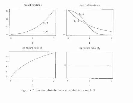
4.7 Survival distributions sim ulated in example 3... 69
4.8 E stim ated log hazard ratios for example 3 w ith n = 500... 69
4.9 E stim ated log hazard ratios for example 3 with n = 10000... 70
4.10 Survival distribution sim ulated in example 6 ... 89
4.11 E stim ated log hazard ratio for example 6 w ith n = 500... 90
4.12 E stim ated log hazard ratio for example 6 with n = 10000... 90
4.13 Survival distribution sim ulated in example 8... 91
4.14 Joint distribution of covariates in d a ta set generated from example 8... 92
4.15 E stim ated log hazard ratios for example 8 with n = 500... 92
4.16 E stim ated log hazard ratio for example 8 with n = 10 000... 92
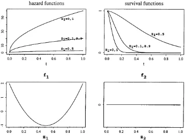
4.17 Survival distributions sim ulated in example 9... 103
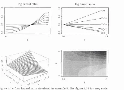
4.18 Log hazard ratio sim ulated in example 9 ... 104
4.19 Grey scale for example 9... 104
4.20 E stim ated log hazard ratio for example 9 with n = 750... 104
4.21 E stim ated log hazard ratio for example 9 with n = 10 000... 105
4.22 Survival distributions sim ulated in example 10... 105
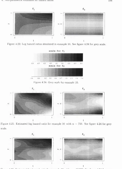
4.23 Log hazard ratios sim ulated in example 10... 106
10
4.25 E stim ated log hazard ratio for example 10 with n = 750... 106
4.26 E stim ated log hazard ratio for example 10 w ith n = 10 000... 106
5.1 E stim ated log hazard ratio from weighted sm ooth of adjusted Schoenfeld residuals for example 1 with n = 500... 120
5.2 E stim ated log hazard ratio from weighted sm ooth of adjusted Schoenfeld residuals for example 1 with n = 10 000... 120
5.3 Log partial likelihood and quadratic approxim ation for example 1... 121
5.4 Survival distribution sim ulated in example 4... 122
5.5 Log p artial likelihood and quadratic approxim ations for example 4 ... 122
5.6 E stim ated log hazard ratio from weighted sm ooth of adjusted Schoenfeld residuals for example 4 with n = 500... 122
5.7 V(^i) and V in example 1, n = 500... 123
5.8 Survival distributions generated in example 5 ... 123
5.9 V(i) and Ÿ in example 5, n = 500... 124
5.10 Various forms of sm oothed Schoenfeld residuals for example 5... 125
5.11 E stim ated log hazard ratio from weighted sm ooth of sim ultaneously adjusted Schoen feld residuals for example 3 with n = 500... 126
5.12 E stim ated log hazard ratio from weighted sm ooth of simultaneously adjusted Schoen feld residuals for example 3 with n = 10000... 127
5.13 E stim ated log hazard ratios for example 3 w ith n = 500 using weighted sm ooth of sim ultaneously adjusted Schoenfeld residuals, weighted sm ooth of individually adjusted Schoenfeld residuals, and sm oothed Schoenfeld residuals... 128
5.14 E stim ated log hazard ratios for example 3 with n = 10000 using weighted sm ooth of sim ultaneously adjusted Schoenfeld residuals, weighted sm ooth of individually adjusted Schoenfeld residuals, and sm oothed Schoenfeld residuals... 129
5.15 E stim ated log hazard ratio from sm oothed adjusted m artingale residuals for exam ple 6 with n = 500... 138
5.16 E stim ated log hazard ratio from sm oothed adjusted m artingale residuals for exam ple 6 with n = 10000... 138
11
5.20 Estim ated log hazard ratios from weighted sm ooths of adjusted m artingale residuals
and from weighted additive regression of adjusted m artingale residuals for example
8 with n = 10000... 141
5.21 Estim ated log hazard ratio from sm oothed adjusted m artingale difference residuals for example 9 w ith n = 750... 149
5.22 Estim ated log hazard ratio from sm oothed adjusted m artingale difference residuals for example 9 w ith n = 10000... 149
5.23 Grey scale for example 9... 149
5.24 Log hazard ratio sim ulated in example 9 ... 149
5.25 Grey scale for example 10... 150
5.26 Estim ated log hazard ratio from sm oothed adjusted m artingale difference residuals for example 10 w ith n = 750... 150
5.27 E stim ated log hazard ratio from sm oothed adjusted m artingale difference residuals for example 10 with n = 10000... 151
5.28 Survival distributions sim ulated in example 11... 152
5.29 Grey scale for example 11... 152
5.30 Residual plots for d a ta set sim ulated from example... 11... 153
5.31 Residual plots for d a ta set simulated from example 11, using Gox models with transform ed or tim e-dependent covariates... 153
5.32 Weighted sm ooth of adjusted m artingale difference residuals for example 11. . . . 154
6.1 Variance of estim ates of /3 and m ean of variance estim ates in 1000 sim ulated d a ta sets from example 1... 157
6.2 Variance of estim ates of /3 and mean of variance estim ates in 1000 sim ulated d a ta sets from example 2... 158
6.3 Variance of estim ates of /3 and m ean of variance estim ates in 1000 sim ulated d a ta sets from example 4... 158
6.4 Variance of estim ates of / and m ean of variance estim ates in 1000 sim ulated d a ta sets from example 6... 159
6.5 Variance of estim ates of / and m ean of variance estim ates in 1000 sim ulated d a ta sets from example 9... 160
6.6 Mean of estim ated log hazard ratio in 1000 sim ulated d a ta sets from example 4 with n = 500, and sim ulated log hazard ratio (dashed line)... 163
6.7 M ean of estim ated log hazard ratio in 1000 sim ulated d a ta sets from exam ple 2 with n = 500 w ith the sim ulated log hazard ra tio ... 164
12
6.9 E stim ated log hazard ratio for example 2 with n = 500, with confidence intervals
and under-sm oothed confidence intervals... 166
6.10 Estim ated log hazard ratio for example 6 with n = 500, with confidence intervals
and under-sm oothed confidence intervals... 166
6.11 E stim ated log hazard ratio for 7th simulated dataset from example 1 with approx
im ate 95% confidence intervals... 169
6.12 E stim ated log hazard ratio for 7th sim ulated dataset from example 1 with approx
im ate 95% global confidence region... 170
6.13 E stim ated log hazard ratio for 2nd sim ulated dataset from example 1 w ith approx
im ate 95% global confidence region... 172
6.14 One hundred functions /? in the 95% confidence region (6.13) for the 2nd sim ulated
d a ta set from example 1 ... 176
6.15 One hundred functions (5 in the 95% confidence region (6.13) for the sim ulated d a ta
set from example 2 ... 177
7.1 Kaplan-M eier estim ates of overall survival in the two treatm ent groups, ABCM and
not ABCM ... 181
7.2 Correlated covariates log2(s/52m) and log2 (serum creatinine)... 183
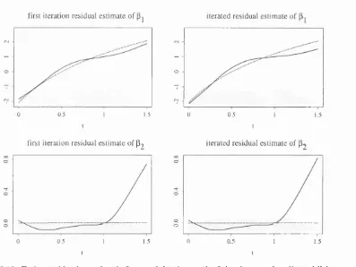
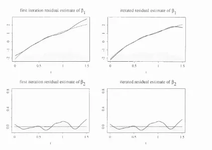
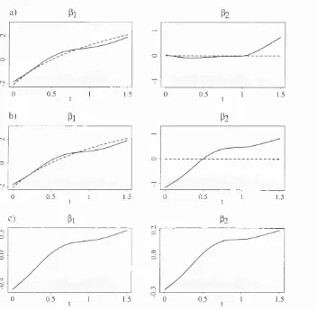
7.3 F irst iteration residual estim ates of log hazard ratios in Cox model with tim
e-varying coefficients with approxim ate 95% pointwise confidence intervals... 185
7.4 F irst iteration residual estim ates of log hazard ratios in m ultiplicative proportional
hazards model w ith approxim ate 95% pointwise confidence intervals... 186
7.5 E stim ated log hazard ratio for log2 (serum creatinine) from sm oothed unadjusted
Schoenfeld residuals... 189
7.6 F irst iteration estim ate of log hazard ratio for log2(s^2m) from weighted sm ooth of
adjusted m artingale difference residuals... 190
7.7 Grey scale for figure 7.6... 190
C .l Iterations of N ew ton’s m ethod, backfitting and diagonalized iteration for finding
least squares estim ates from sim ulated d a ta w ith p = 2... 207
C.2 Iterations of N ew ton’s m ethod, backfitting and diagonalized iteration for finding
13
List o f Tables
6.1 P roportion of pointwise confidence intervals which include sim ulated value of fi{t)
in 1000 sim ulated d a ta sets from example 1 with n = 500... 161
6.2 P roportion of pointwise confidence intervals which include sim ulated value of f { t , z)
in 1000 sim ulated d a ta sets from example 9 with n = 750... 162
6.3 P roportion of pointwise confidence intervals which include sim ulated value of P{t)
in 1000 sim ulated d a ta sets from example 4 with n = 500... 163
6.4 Proportion of pointwise confidence intervals which include sim ulated value of /3{t)
in 1000 sim ulated d a ta sets from example 2 w ith n = 500... 164
6.5 Proportion of pointwise confidence intervals which include sim ulated value of / ( z )
in 1000 sim ulated d a ta sets from example 6 w ith n = 500... 165
6.6 P roportion of pointwise confidence intervals with undersm oothing which include
sim ulated value of P{t) in 1000 sim ulated d a ta sets from example 2 w ith n = 500. 167
6.7 Proportion of pointwise confidence intervals w ith undersm oothing which include
sim ulated value of /3{t) in 1000 sim ulated d a ta sets from example 6 with n = 500. 167
6.8 P roportion of pointwise confidence intervals which include sim ulated value of P{t)
for all t in the range of estim ation in 1000 sim ulated d a ta sets from example 1. . 168
6.9 Proportion of global confidence intervals which include sim ulated value of /3{t) for
all t in th e range of estim ation in 1000 sim ulated d a ta sets from example 1. . . . 170
6.10 P roportion of confidence regions (6.13) which include sim ulated function (3 in 1000
sim ulated d a ta sets from example 1... 174
6.11 P roportion of confidence regions which do not include any constant (3 in 1000 sim
ulated d a ta sets from example 1... 175
7.1 Sum m ary of prognostic variables... 182
7.2 Cox proportional hazards model ... 184
7.3 Minimum values of (/3^ - /5)^(T^(/3^)“ (/3^ - /3) for constant indicating inclusion
14
7.4 Minimum values of (/^ - - / ) for linear / , indicating inclusion in
confidence regions as in (6.13)... 186
7.5 Cox model with tim e-dependent and transform ed covariates resulting from residual
15
C hapter 1
In trod u ction
Analysis of censored survival data, for example from a clinical trial, typically involves estim at
ing association between covariates and the hazard function. The Cox model (Cox, 1972) allows
estim ation of the hazard ratio as a param etric function of covariates. Although th e Cox model
is sem i-param etric in the sense th a t the baseline hazard function is unspecified, the hazard ratio
has a fixed param etric form with respect to covariates, and is assumed to be constant in time. As
w ith any param etric model, this assumed form is often inappropriate, and m ethods are needed for
checking th e model cissumptions, exploring alternatives, and presenting flexible estim ates. The
next section gives an illustrative example in ordinary regression and the following sections describe
th e aims, approach and context of this thesis, w ith an outline of the content in section 7.
1
A n exam ple in ordinary regression
To illustrate the aims of this thesis, this section describes the simple problem of estim ating the
relationship between the mean of an observable random variable and a continuous covariate.
Typically a regression model is used, with residual analysis to explore w hether a linear or some
other, possibly non-param etric, model for the m ean function is m ost appropriate.
To illustrate this explicitly, d a ta were sim ulated for 500 independent and identically distributed
observations { X , Y ) , X generated from a uniform distribution on [0,1], and Y generated from a
norm al distribution with m ean { X — 1/2)'^I { X > 1/2) and standard deviation 0.1. Figure 1.1
1. Introduction 16
o
0.0 0.2 0.4 0.6 0.8 1.0
Figure 1.1: S catter plot of simulated d ata with ordinary least squares linear regression line.
o
-a o
o
0.0 0.2 0.4 0.6 0.8 1.0
Figure 1.2: Residuals from linear model with smoothing spline smooth and approxim ate 95%
pointwise confidence intervals. (Note th a t the vertical scale is not the same as in figure 1.1)
The form of the relationship is not clear from the scatterplot, and initially a linear model was
used. A coefficient of 0.21 was estim ated, with standard error 0.02; the estim ated mean is shown
on figure 1.1. Since there is no reason to assume th a t the association is linear, residual analysis
was carried out; figure 1.2 shows the residuals from the fitted linear model plotted against the
covariate. The solid line shows a smoothing spline smooth, with 5 degrees of freedom, and the
dotted lines show approxim ate 95% pointwise confidence intervals for the smooth (see Hastie and
Tibshirani (1990b) for smoothing splines and their standard errors). The residual plot shows the
non-linearity and indicates a more appropriate form. As a result a model might be chosen allowing
different slopes for small and large values of X , and with quadratic term s as well as linear.
Alternatively, a sm ooth but flexible estim ate of the association between the observation Y and
1. Introduction 17
d
(N d
o
d
(N d
0.0 0.2 0.4 0.6 0.8 1.0
Figure 1.3: Smooth estim ate of E { Y | X ) with approxim ate 95% pointwise confidence intervals.
the d a ta with a sm oothing spline smooth and approxim ate 95% confidence intervals. This figure
also shows the non-linearity, and indicates the underlying form. In fact the sm ooth in figure 1.3
is exactly the same as the smooth in figure 1.2 plus the linear estim ate from the fitted model.
The smooth is a penalized least squares estim ate of the mean, and a consistent estim ator as long
as the underlying mean is a smooth function and the degrees of freedom of the sm oother used to
estim ate it are increased at a suitable rate as the sample size increases (Gu & Qiu, 1994).
These plots and estim ates are all easy to produce in existing statistical packages, in particular
S-Plus, see appendix H.
2
N on-param etric and residual analysis in hazard estim a
tion
The approach to modelling illustrated in section 1 provides simple and intuitive m ethods of explor
ing and estim ating the association between the observation and the covariate. The relationship
between different (param etric and non-param etric) estim ates is clear, results are easy to interpret
and estim ates are easy to calculate in existing software. This thesis is concerned with developing
the corresponding approach to estim ating the relationship between a hazard ratio and covariates
from censored survival data.
F irst, this section describes the problems in this approach when estim ating a hazard ratio from
censored survival d a ta instead of a mean from independent and identically distributed observa
1. Introduction 18
In addition to any dependence on covariates, a hazard ratio is a function of time, so estim ating the
dependence of the hazard ratio on continuous covariates means estim ating a function of a t leaist
two continuous variables. Therefore a fully non-param etric approach is difficult in practice and
often infeasible. N on-param etric estim ators have been developed in various models which reduce
the dimension of the hazard ratio function by making some assum ptions bu t leaving other aspects
unspecified. As a result there are several ways of estim ating the hazard non-param etrically and it
is difficult to com pare different estim ates and model assumptions. The estim ates are also difficult
to calculate, both in term s of the feasibility of the calculations and the ease with which they can
be found in existing statistical software.
Models such as the Cox model make assum ptions both on the dependence of the hazard on
tim e and on the dependence of the hazard on covariates. Therefore, when checking models and
exploring alternatives, there is more th an one possible alternative and it may not be clear which
of the assum ptions is inappropriate. Residuals from the Cox model are easy to calculate bu t
difficult to interpret. In an ordinary regression model, the system atic variation in the m ean and
the random variation are w ritten as separate components of the observation, V = f { X ) + e where
e has m ean zero, enabling excess system atic variation in the m ean to be analysed using residuals
f { X ) — f { X ) + e. In contrast a hazard function determines both the system atic and random
variation in survival and there is no residual with an obvious interpretation in term s of random
and excess system atic variation. There are several ways of calculating residuals and i t ’s not easy
to see which m ethod should be used, or for what.
In the ordinary regression example in section 1, the two approaches to exploratory analysis for
choosing and checking models (ie. non-param etric estim ation and residual analysis) are basically
the sam e and therefore combine the advantages of each approach. In survival analysis, on the
other hand, the relationship between non-param etric estim ates and residual analysis is not so
clear. N on-param etric estim ates have useful asym ptotic properties, but they are not easy to use
in a practical analysis and they are difficult to interpret in the context of com paring different
models. On the other hand, residuals are easy to calculate and more clearly relate more and less
restrictive models, bu t they have unknown properties; they are not necessarily consistent estim ates
of anything useful and i t ’s not clear w hat they are approxim ating.
This thesis makes use of the relationship between non-param etric estim ation of hazard ratios and
Cox model residual analysis, using residual m ethods to find easy ways of calculating consistent
estim ates, and using the theory for non-param etric estim ates to study the properties of (even
easier) residual plots. The result is estim ators which are easy to calculate, have known and useful
1. Introduction 19
hazard ratio.
Specifically, the aims of this thesis are
• to review and extend results on consistent non-param etric estim ation of the hazard ratio;
• to find m ethods of calculating consistent non-param etric estim ates th a t are easy to use and
reliable;
• to find m ethods based on residuals available in existing software which approxim ate consis
ten t estim ates w ith useful properties;
• to deduce guidelines for residual analysis and its interpretation.
3
C on text and notation
T he context throughout this thesis will be survival d a ta with right-censoring. Survival tim es for n
individuals will be T i, . . . , T„ which will be equal to either the observed tim e of death or th e time
of censoring; Si is the indicator of Ti being an observed time of death. Individual i has covariate
vector Zi, of length p, which may change over time, although in some places the covariates will
be assum ed to be fixed from time zero. The triples {Zi,Ti,Si) will be independent and identically
distributed.
T he sam ple size n will be assumed to be reasonably big to make exploratory analysis w orth while.
Since the fiexibility of estim ates can only be increased slowly as the sample size increases, very
little fiexibility will be possible if there are less than, say, 100 individuals. Illustrations will be
based on a d a ta set from a study of myelomatosis with ju st over 1000 individuals (chapter 7) and
sim ulated d a ta sets of 500 or 750 individuals.
T he counting process notation of Aalen (1978) will also be used; A^i,. . . , and T i , . . . ,1 ^ are
defined as Ni{t) being equal to 1 if individual i has survival tim e T{ < t and = 1, and zero
otherwise; Yi{t) is 1 if t and zero otherwise. Thus Ni counts the num ber of deaths observed
so far for individual i and Yi indicates whether or not they are at risk. However only one d eath is
allowed per individual, so th a t Ni is always equal to 0 or 1, and individuals are not allowed to be
a t risk a t any tim e after death or censoring.
By this definition Ni is right-continuous with left-hand limits and Yi is left-continuous w ith right-
1. Introduction 20
also. Let T be the history process for the n individuals, T t consisting of the values of Ni{u), Yi{u)
and Zi{u) for i = 1 , . . . , n and all u < t . Then since Yi and Zi are left-continuous, Yi and Zi are
predictable w ith respect to T .
It is assumed throughout th a t the uncensored survival tim e for individual i has a continuous
distribution with hazard ra te \ i and cum ulative hazard A^, A*(() = Ai(u)du. Also independent
censoring is assumed, in the sense described in Andersen et al. (1991) section II. 1, so th a t the
counting process Ni has intensity process given by
l i m s t io ^ { N i ( t + St) - Ni {t ~ ) | J ^ t -} /S t = Yi{t)Xi{t).
This ensures identifiability of the distribution of Ti in inference from observations on {Ni, Yi), see
for exam ple Fleming & H arrington (1991) page 26. It also means th a t Ni{t) — Yi{u)Xi{u)du is
a local square integrable m artingale — see Andersen et al. (1991) section II.4.
T he h azard function for individual i is and will be assumed to depend on tim e and the covariate
vector for individual i as
Xi{t) = X{t,Zi{t)}.
Note th a t this makes the assum ption th a t if individuals have the same covariate vector a t time t
then they have the same hazard at tim e t. The aim is to estim ate the function A, which has p + 1
variables.
In general it is assumed th a t the survival distributions are continuous so th a t two uncensored
individuals can only have the same survival tim e with probability zero. In practice the m ethods
should be equally useful in d a ta sets with a small num ber of tied survival times, for exam ple due
to rounding. For example ties occur in the myeloma d a ta analysed in chapter 7 when survival
tim es are rounded to whole weeks. For simplicity notation will often apply only to d a ta w ithout
tied survival times; extension to d ata with ties should be fairly obvious.
Let d be the num ber of observed events, which will be indexed by {i), and occur at tim es i(i) <
< ; Z(i) is the covariate for the individual observed to die a t . And let TZ{t) denote the
risk set a t tim e t, 'JZ{t) = {i : Yi{t) = 1}. Then there are two equivalent notations, which will be
convenient in different places; for a function of tim e, / ,
/
Y^f{t)dNi{t) =
YI
f{t{i))]
t=i events (i)
and if f i is a function of tim e for each individual i.
Y,Yi{t)Mt)= YI
1. Introduction 21
Note this notation assumes th a t there are no ties, a single observed death a t each A further
subscript can be introduced if there are ties, bu t is not used in this thesis.
4
Hazard ratios and partial likelihood
The Cox model (Cox, 1972) formulates the hazard X{t, z) as the product of a baseline hazard Xo{t)
and a hazard ratio. The baseline hazard function Aq is unspecified and is not estim ated, while the
hazard ratio is estim ated according to the param etric form in the Cox model. T hroughout this
thesis a sim ilar form will be used,
X{t, z) = Ao(t) e x p { /(i, z)] (1.1)
where to make the model identifiable, / has some constraint such as / ( ( , 0) = 0 for all t. E stim ates
are developed for the log hazard ratio / , with the baseline hazard Aq rem aining unspecified.
U nder the general model (1.1), Cox’s partial likelihood (Cox, 1975) can be w ritten as
r / f . TT ex p (/(t(i),Z (i))}
observed L t h s «) '
T his can be used w ith various forms for / to estim ate the hazard ratio w ithout estim ating or
restricting the baseline hazard Aq. Thus, although effects to be estim ated m ust necessarily be
restricted by either a param etric form, or some smoothness constraint, the underlying survival
distribution does not affect the estim ation. T he form (1.1) also avoids the problem of negative
hazard estim ates.
One advantage of w riting the hazard as in (1.1) is th a t a m ultiplicative model can be used when
th e dimension of the covariate vector, p, is more th an one,
A(t, z i,...,Z p ) = A o (i)e x p { /i(i,z i) + ■ ■ - + fp{t,Zp)}. (1.2)
In practice, some such model is vital to reduce the dimension of the hazard ratio from p + 1 , and
this form allows the effect of each covariate to act m ultiplicatively on the hazard, which in many
situations may be the m ost biologically plausible. An alternative would be to have th e effects of
covariates acting additively on the hazard function as in Aalen’s model (1989). A lthough this thesis
is based on the m ultiplicative hazards model, m ethods apply even more easily to additive hazards
models (see for example chapter 5 section 2.5). M ethods for choosing between m ultiplicative and
additive hazards have been developed by McKeague & Utikal (1991) and Gr0nnesby & Borgan
1. Introduction 22
O ther alternatives to (1.1) include accelerated failure tim e models (Kalbfieisch & Prentice, 1980,
chapter 6), (Cox & Oakes, 1984, section 5.2) and param etric survival models such as Weibull
and log-logistic regression models (Kalbfieisch & Prentice, 1980, page 31), (Cox & Oakes, 1984,
section 6.3) and, more generally, the generalized gam m a model (Farewell & Prentice, 1977). Choice
between the sem i-param etric model (1.1) and various param etric models is discussed by M arubini
& Valsecchi (1995, page 290), Gore et al. (1984) and Lin & Spiekerman (1996). Therneau et
al. (1990, appendix 3) discuss the application of model checking m ethods based on m artingale
residuals to param etric models.
E stim ation of the hazard ratio is natural in any context in which the aim is to determ ine the
effect of covariates on survival, ra th e r th an to determ ine the value of the hazard itself. In such a
context estim ation of the hazard X{t,z) for each value of z would in any case need to be followed
by further m ethods to compare hazards for different covariate values. On the other hand, for
clinical interpretation of covariate effects it will norm ally be necessary to eventually estim ate the
baseline hazard function, or ra th e r the cumulative baseline hazard function, as well. This should
in general be possible using an estim ator similar to Breslow’s baseline hazard estim ator for the
Cox model (Breslow, 1974), and is not considered further here.
5
C onstraints on non-param etric estim ates — sm ooth in g
Clearly some constraint is needed when estim ating a continuous function from a finite sample.
To find sensible non-param etric estim ates of continuous functions from finite sam ples, estim ates
are forced to be sm ooth — a num ber of different m ethods of sm oothing are used throughout this
thesis and they are described in appendix A.
T he sm oother the estim ate is made, the lower i t ’s variance will be, bu t th e higher th e bias will be
if the function being estim ated is not really th a t smooth. The aim is to choose a level of sm oothing
th a t keeps both the bias and the variance small, see H astie & Tibshirani (1990b) section 3.3. For
th e purpose of asym ptotics the smoothness should be reduced at a suitable rate as the sam ple size
increases so th a t both th e bias and variance are reduced.
As an alternative to sm oothing, cumulative (or integrated) non-param etric estim ates can be used.
These have the advantage of nicer theoretical properties, in particular faster {y/n) asym ptotic
convergence due to differentiability of the corresponding functional of th e probability m easure
(van der V aart, 1991), and avoid the arbitrariness introduced by choosing a sm oother. They are
1. Introduction 23
easy to interpret in the context of the form of the relationship between the hazard ra tio and
covariates, and are not very helpful for suggesting and exploring models. The m ethods developed
in this thesis therefore concentrate on estim ating sm oothed hazard ratios and not cum ulative or
integrated hazard ratios.
Asym ptotic considerations govern the ra te a t which the smoothness decreases as the sam ple size
increases. For choosing smoothness for a specific d a ta set, m ethods such as cross-validation might
be used, with the purpose of finding some optim al smoothness depending on the data, as described
in H astie & T ibshirani (1990b) section 3.4. Such m ethods are not developed here and sm oothness
is assum ed throughout to be chosen in advance.
6
M od els for d ependence on tim e and covariates
The log hazard ratios f i { t , z i ) ,. . . , f p { t , Z p ) in (1.2) depend on both tim e and covariates, so non-
param etric estim ation can mean non-param etric in t , in z, or in both t and z. Similarly checking
model assum ptions can mean checking the form with respect to t , checking the form w ith respect
to z, or checking the form with respect to t and z. Therefore throughout this thesis estim ation
will be considered in the context of three different models. Firstly, a model where the log hazard
ratio is param etric (linear) in the covariates, bu t the coefficients are unspecified functions of time,
the ‘Cox model with tim e varying coefficients’,
A(f,z) = Ao(f)exp{/3i(<)zi H h Pp{t)zp}. (1.3)
This model would m ake no assumptions on A if there was only a single binary covariate. It can
be used with a non-linear, but specified, form by first transform ing covariates.
In th e second model, the log hazard ratio is assumed to be constant in time, bu t is an unspecified
function of each covariate, the ‘m ultiplicative proportional hazards m odel’,
A(f,z) = A o(f)exp{ /i(zi) -f • • • -I- f p { z p ) } . (1.4)
Here, hazard ratios th a t are non-constant in tim e can be included, if the form w ith respect to tim e
is specified, using tim e-dependent covariates. Note th a t, confusingly, this model is also called an
additive model due to the additive form in the exponential.
T he th ird model for A assumes nothing but the m ultiplicative form for m ultiple covariates; for
each covariate the log hazard ratio is an unspecified function of both tim e and the covariate, the
‘m ultiplicative hazards m odel’,
1. Introduction 24
Each model is of course useful in different contexts.
7
C on ten ts and outline o f thesis
The following two chapters are reviews of the literature on residual analysis for th e Cox model
and on non-param etric hazard models. Although there is necessarily considerable overlap between
the two, m ost of the literature approaches the problem either as checking the Cox model, or as
estim ating the hazard or hazard ratio w ithout any use of the Cox model, so the two approaches
are reviewed in separate chapters.
C hapter 4 contains development of non-param etric estim ation in each of the three models (1.3),
(1.4) and (1.5). The Cox-model with time-varying coefficients (1.3) is developed in section 2.
E stim ation is discussed and relevant estim ators from the literature are sum m arised in a common
fram ework in section 2.1, with discussion of iterative m ethods for finding them in section 2.2.
Section 2.3 deals w ith asym ptotics, and contains the main theoretical results for this model —
asym ptotic results are only available in the literature for estim ators th a t would not usually be used
in practice, and here consistency is shown for more useful estim ators using regression sm oothing
and local estim ation. The results are in theorems 4.1 and 4.2 on page 64. E stim ation is illustrated
w ith sim ulated examples in section 2.4.
T he m ultiplicative proportional hazards model (1.4) is developed in section 3 of chapter 4. Again
relevant estim ators from the literature are summ arised in a common framework. Section 3.2 is
concerned with iterative m ethods for finding estim ates; while the usual N ew ton’s m ethod can
involve excessive com putation, theorem 4.3 (page 87) shows th a t an alternative m ethod can be
used which is both simpler and com putationally more feasible — under usual conditions, and
startin g from a suitable initial value, the iteration will arrive at the desired estim ate. Section
3.3 sum m arises results on consistency from the literature, and sim ulated examples are shown in
section 3.4.
Section 4 of chapter 4 develops the m ultiplicative hazards model (1.5). New estim ators are pro
posed in section 4.1, and a feasible iterative m ethod for finding estim ates is found in section 4.2.
Use of the model and presentation of estim ates is illustrated in section 4.4 in sim ulated examples.
C hap ter 5 introduces the use of Cox model residuals and their relation to the non-param etric
models of chapter 4, and the iteration of residual estim ation. C hapter 5 is also divided into
1. Introduction 25
non-proportional hazards, or the Cox model with tim e-dependent coefficients (1.3). Residual
estim ates, and iterated residual estim ates, are proposed in sections 2.1 and 2.2 — at the first
iteration, the estim ates use a combination of the m ethods in the literature. Section 2.3 contains
theoretical results for the iterated estim ates, specifically th a t under suitable conditions and using
appropriate m ethods, iteration of residual estim ates leads to consistent estim ators of the time-
dependent coefficients, similar to the non-param etric estim ates in chapter 4. Sections 2.4 -2 .7
discuss the im plications of the results for practical residual analysis. It is shown th a t one p articular
m ethod of residual analysis is both easy in existing software (S-Plus) and obtains estim ates with
good, if approxim ate, theoretical properties. Some m ethods th a t are proposed in the recent
lite ratu re are shown to be inferior. These results are illustrated using sim ulations in section 2.8.
Section 3 of chapter 5 gives a similar development for the estim ation of non-log-linear form in the
Cox model, or the multiplicative proportional hazards model (1.4). Estim ates based on (different)
Cox model residuals, and iteration, are proposed in sections 3.1 and 3.2. Again at the first iteration
the estim ates are similar to those suggested in the literature, bu t a new residual m ethod for
m ultiple covariates is introduced in equation (5.14) (page 133). Section 3.3 contains the theoretical
results th a t iteration of residual estim ation leads to the consistent estim ates of chapter 4. The
practical im plications for residual analysis are discussed in section 3.4. Again the theoretical
results show th a t residual analysis as proposed leads to estim ators th a t have desirable theoretical
properties, and are available w ithout further program ming from S-Plus, while some m ethods
recently proposed in the literature have less desirable properties. The m ethods are illustrated in
sim ulations in section 3.6.
Section 4 of chapter 5 develops residual analysis for the im portant situation where neither propor
tional hazards, nor a known functional form for continuous covariates, can be assumed w ithout
checking. This is the most likely situation in m any practical contexts b u t currently hardly any
m ethods are available th a t take this situation into account; those th a t do (see chapter 2) need
developm ent to be useful in practice and involve extensive program m ing and com putational effort.
In section 4.1 a new type of residual estim ate is introduced which can be used to check the Cox
model against a very general alternative, while still presenting inform ation on specifically w hat
alternative is needed. Residual estim ates are related to the non-param etric estim ates of chapter
4, giving theoretical justification for use in a practical analysis. Im plem entation in S-Plus is not
im m ediate for this approach, but still quite reasonable, as discussed in section 4.6. P ractical issues
are discussed w ith sim ulated examples in section 4.7.
C hapter 6 is concerned with confidence intervals and inference for the estim ates of chapters 4
1. Introduction 26
confidence intervals are m ostly left for future work, with heuristic justification presented in this
chapter. Variance estim ates are reviewed or suggested, discussed, and illustrated in section 2, and
in section 3 the coverage of pointwise confidence intervals is investigated in sim ulation studies.
The problem of low coverage due to bias in sm ooth estim ates is discussed and solutions from
generalized additive models are applied. In section 4 global confidence intervals are developed,
again applying solutions from generalized additive models, while section 5 discusses problem s of
inference for the form of a function and suggests m ethods for visualising global confidence regions.
C hapter 7 is a practical analysis of d a ta from the Medical Research Council’s trials on myeloma.
While these trials have been analysed in the medical literature and the questions they set out
to answer have basically been answered, it is clear th a t there is considerable inform ation to be
found from the d a ta which has not been m ade use of due to a lack of suitable statistical methods.
C hapter 7 presents an analysis of these d a ta using the m ethods developed in this thesis.
Appendices A -E sum m arise general m ethods and results which are used specifically in various
p arts of th e thesis. Since one of the m ain aims of this thesis is to find m ethods of estim ation
which are easily im plemented in existing software, S-Plus code, and where necessary, new S-Plus
27
C hap ter 2
R ev iew o f residual analysis
1
In trod u ction
T he Cox proportional hazards model (Cox, 1972) has been very widely used to analyse survival
d ata, in p articular in medical applications. Residuals were proposed when the model was first
used, eg. Kay (1977), and have developed a lot since. This chapter gives a review of residual
m ethods developed so far.
T he basic form of the Cox proportional hazards model says th a t the hazard at tim e t for an
individual w ith covariates Z is with
\{t, z) = Xo{t) exp(/)^z) (2.1)
for a constant vector of param eters /3. The log partial likelihood of Cox (1975) is
dNi{t).
^oo / r ^
i = l ”' 0 \ '-j=l
T he coefficient /3 is usually estim ated by maximizing 1{P)] let P be the m aximum p artial likelihood
estim ate. Also the baseline cumulative hazard function Ao{t) = Ao(u)du is estim ated by the
Breslow estim ate (Breslow, 1972),
" S i
E U
(2.2)T he p artia l likelihood score function is
2. Review of residual analysis 28
and the score derivative is
- m = t [ (2.3)
where
5W(t,/3) =
3=1
j = l
= ^ ' £ Y i { t ) Z j ( t ) « ^ e x p { 0 ^ Z j { t ) } , (2.4)
" 3 = 1
and for a column vector z, = z z ^ .
Under the model (2.1) and appropriate conditions, /3 converges asym ptotically to the true /3. Its
variance, X{P)~^, is estim ated by I 0 ) ~ ^ , and Ao(t) converges to Ao{t) (Andersen & Gill, 1982).
T he following section gives a list of the m ain types of residuals th a t have been suggested for the
Cox model; variations of each type have been used for various purposes. Sections 3 - 7 look at
residual analysis for checking various aspects of the model and estim ation.
2
R esiduals for th e Cox m odel
2.1
C rude residuals
The first residuals to be used with the proportional hazards model are based on th e general,
or ‘crude’, residuals of Cox and Snell (Cook & Weisberg, 1982, page 177). T heir use w ith the
proportional hazards model was suggested by Crowley & Hu (1977) and Kay (1977). They are
the fitted values of the cumulative hazard for each individual,
Èi = exp(^^Z<)Âo(Ti) (2.5)
where Aq is the Breslow estim ate (2.2). The residual Ei is equal to the estim ated cum ulative hazard
for individual i evaluated at Ti. The values of the cumulative hazard function, exp(^^Z i)A o(T i),
form a (censored) sam ple from a unit exponential distribution, so under the assumed model, the
estim ated values Ei might be expected to behave like unit exponential variables. They have been
used to assess th e overall fit of the model, as discussed in section 3, and to check the form of the
2. Review of residual analysis 29
having undesirable properties, and being inferior to other types of residual, following (see sections
3 and 6).
2.2
M artin gale residuals
M artingale residuals were first suggested by Barlow & Prentice (1988) as a special case of their
generalized residuals (see section 2.5) and studied more specifically by Therneau, Grambsch &
Flem ing (1990). The m artingale residual Mi is given by
Mi
fOO
= / dNi{u) - yî(u) exp(/3^Zi)dÂo(u) = Si - Èi. Jo
The m artingale residual Mi is then the observed num ber of events for individual i minus the
expected num ber under the fitted model and conditional on the observed covariate value Z*. As
a result they are useful for checking the form of the model with respect to the covariates; several
types of adjusted and transform ed m artingale residuals have also been used, see section 6.
2.3
S ch o en feld ’s partial residuals
Schoenfeld (1982) introduced a type of residuals based on the covariate value corresponding to an
observed event minus the conditional expected value of the covariate under the fitted model;
for observed event (%), with as defined in (2.4). Each residual is a p-vector and there
is a residual for each observed event ra th e r th a n for each individual. In contrast to m artingale
residuals, Schoenfeld’s residuals give the observed minus expected value of the covariate a t the
event times, conditional on the risk sets, and correspondingly they have been used to assess the
form of th e model with respect to time, th a t is, the proportional hazards assum ption, as seen in
section 7.
2.4
Score residuals
A nother type of residual for the Cox model is the score residual . These are defined as
Si = r { Zi(t) - [ d N M - Yi(t)exp{4^Zi(t)}dAo(t)].
2. Review of residual analysis 30
with and defined in (2.4) and where Aq is the Breslow estim ate (2.2) (Therneau et ai,
1990). They are similar to Schoenfeld residuals; each residual Si is a p-vector, bu t they are defined
for individuals not observed events. They are useful for assessing influence, see section 5.
2.5
G eneralized residuals
Barlow and Prentice (1988) suggested a generalized form for residuals for the Cox model, which
includes m artingale residuals, Schoenfeld residuals and score residuals and makes it easier to see
the likely uses and properties of each type of residual. They define a generalized residual for
individual i a t tim e t as
fi{t){dNi{t) - Yi{t) ex p0' ^Z i )dAo{t )} (2.6)
for predictable processes fi, estim ated by fi.
Since dNi{t) and dAo{t) can be non-zero only at observed event times t, this gives a residual for
each individual at each event time — n d residuals. These are then summ ed over the events to
give a generalized m artingale residual for individual i,
rOO
/ (2.7)
Jo
or summed over the individuals to give a residual for (a single) observed event (i).
They can also be summed over both individuals and events a t the same time, or over subsets of
th e individuals or subsets of the events.
If f i is taken to be 1, and summing over the events, then (2.7) is the m artingale residual Mi. If f i is
taken to be Zi and summing over the individuals, then (2.8) is the Schoenfeld residual for event (i).
If /^(i) = Zi{t) — {t, P) / $ ) and summing over the events, then (2.7) is the score residual
Si. From this representation it seems natural to use m artingale residuals (which are generalized
residuals summed over time) to check the form of the model w ith respect to covariates, and to use
Schoenfeld residuals (which axe generalized residuals summed over individuals) to check the form
w ith respect to time. Score residuals include a m easure of the difference between a covariate value
for an individual and an average covariate value, so can be expected to be useful for assessing
2. Review of residual analysis 31
2.6
D ev ia n ce residuals
T herneau, Grambsch & Fleming (1995) also define deviance residuals, m otivated by deviance
residuals from generalized linear models,
di = s ig n (M i)v ^ { -M j - 6^ log(J«
-They are a transform ation of the m artingale residuals which results in a less skewed distribution
and therefore they have been suggested to be used to detect individual outliers, however they have
been little used in practice and have not been found to be particularly useful, see section 4 .
3
A ssessin g th e overall fit o f th e Cox m odel
As m entioned in section 2.1, crude residuals Ei estim ate the cumulative hazards for individuals i
evaluated a t Tj, which form a censored sample from a unit exponential distribution. Consequently,
early developm ents of residual analysis for the Cox model included plotting the survival curve of
the crude residuals as a check of the overall fit of the model (Crowley & Hu, 1977; Kay, 1977).
However Lagakos (1981), Crowley &: Storer (1983) and B altazar-A ban & P ena (1995) show th a t
due to estim ating Aq, and in particular because the function Aq is completely unspecified, the
d istribution of the Ei S is not necessarily w hat would be expected. For example if no covariates
are in the model, Aq can be m ade to ‘fit’ the d a ta exactly; the order statistics of the residuals
are then exactly the order statistics of the (censored) unit exponential distribution, and give no
inform ation about the fit of the model. Furtherm ore even if these plots could indicate th a t the
Cox model is inappropriate, they cannot indicate in w hat way.
4
A ssessin g m odel adequacy for individuals
T herneau, Gram bsch & Fleming (1990) have suggested using deviance residuals to detect individ
ual outliers. A large positive value of the residual indicates an individual dying too soon according
to the model, and a large negative value indicates an individual living too long, while the tra n s
form ation from the m artingale residuals ensures th a t the residuals have a reasonably sym m etric
and even spread if the model applies to each individual (Therneau et al., 1990). However they
have found little use in practice, and in fact indication of individual outliers may be considered of
2. Review of residual analysis 32
form of the model used.
5
Influence residuals
In general regression models influence residuals have been developed using pertu rb atio n of the
model (Cook & Weisberg, 1982); a particularly simple form of influence residual is the jackknife
residuals which measure the difference in the estim ate P due to each observation — /3 —
where is the coefficient from the model fitted w ithout observation i. For the Cox model,
jackknife residuals are not ideal as their calculation involves fitting n + 1 models individually.
Score residuals have been found to approxim ate jackknife residuals, if suitably adjusted, and to
be useful for assessing influence in various forms.
5.1
A d ju sted score residuals
Cain & Lange (1984) and Reid & Crèpeau (1985) suggested scaled score residuals,
îi =
These are derived as approxim ations to the jackknife residuals using a weighted score m ethod by
Cain & Lange and using the empirical influence function by Reid & Crèpeau. Storer & Crowley
(1985) suggest a similar, bu t not identical, approxim ation to A/?i based on one-step augm ented
regression model diagnostics. The jackknife residuals and the two approxim ations are com pared
by T herneau, Grambsch & Fleming (1990). F urther approxim ations are made by P e ttitt & Bin
D aud (1989b).
5.2
S in gle m easures o f case influence
One problem with the adjusted score residuals described above is th a t there is a set of residuals
associated w ith each covariate. Often it is desirable to have a single overall m easure of influence for
each individual. P e ttitt & Bin Daud (1989a) apply the likelihood displacement m ethods of Cook
(1986) for ordinary likelihood models, and with an approxim ation obtain the influence residuals
Sj^îi = —S j ' X 0 ) ~ ^ S i . Again P e ttitt & Bin Daud (1989b) have a further approxim ation. Barlow
(1997) develops this m ethod further to apply to models for multiple failure times and Ccise-cohort