F I N A N C I A L F R A G I L I T Y
I N A B A S I C A G E N T – B A S E D M O D E L
Guido Fioretti Università di Siena Centro Sistemi Complessi
1. Introduction
The concept of financial fragility is intriguing for the modeller because in spite of a long history of verbal theory (Minsky 1982), little has been done in the field of mathematical and computational economics. Surely, one of the reasons is that financial fragility involves heterogeneity of economic agents, structures of interactions and intricate feed-backs between banks, firms and institutional agents. As it has been noted, any theory of the formation and diffusion of the avalanches of bankruptcies that affect capitalist economies with unpredictable timing should begin with a characterisation of the structures of credit obligations (Shubik 2004). Unfortunately, structures are wiped off by aggregate macroeconomic models.
This contribution originates from the observation that a rather recent development in the art of computer programming may constitute a precious tool in order to model financial fragility. Indeed, object-oriented programming – so the name of the technique – triggered a cascade of applications of computer-based simulations to the social domain that is not showing any sign of resting. Computer models of social systems based on object-oriented programming are called agent-based models. A brief explanation of their functioning is in order.
that generate “deterministic chaos” constitute a paramount example of a field where hardly anything could have been said had computers not been available.
Agent-based simulation models constitute a further development of the possibilities offered by computing machines, in that aggregate equations no longer constitute the point of departure. Rather, the idea is to describe the behaviour of single components of a system – e.g. economic agents in an economic system – and reconstruct the aggregate behaviour by simulating their interactions. In this way, agent-based computer modelling develops features that are in many respects intermediate between those of verbal descriptions and those of equations-based models (Gilbert and Terna 2000).
Agent-based models make macroeconomic features emerge out of microeconomic behaviour that may produce different outcomes depending on the timing and permissions by which interactions take place. In this sense, the agent-based modelling philosophy is just opposite to that of the “representative agent”, as well as to the practice of deriving aggregate behaviour by simple summation of individual contributions.
Financial fragility is an interesting subject for agent-based models. In fact, financial fragility is about chains and cascades of bankruptcies caused by intricate structures of liabilities in an environment where a huge number of heterogeneous agents operate.
The market for inter-bank loans has been a fruitful subject of investigation of the possibility of cascades of exposures that are in many respects an instance of the more general phenomenon of financial fragility (Iori and Jafray 2001; Iori 2004; Iori, Jafray and Padilla 2005). These studies have highlighted that if banks are homogeneous in terms of size and exposure to risk, then the inter-bank market has a strong enough stabilising effect to make avalanches impossible. On the contrary, avalanches are possible if banks are sufficiently heterogeneous.
My contribution aims at exploring the possibility of financial fragility in a more general environment, a theoretical framework developed by Vercelli (2000) where economic agents lend money to one another. By means of a simple agent-based model, I wish to highlight sufficient conditions for a financial system to be fragile.
of the state space. However, avalanches are still not there. Section 5 highlights that by adding the additional constraint of fiduciary stable relationships between lenders and borrowers avalanches of bankruptcies may take place. Finally, section 6 concludes with an evaluation of the relationship between this agent-based model and equations-based models based on the same theoretical framework.
2. The Framework
The framework proposed by Vercelli (2000) is simple and abstract. Essentially, a collection of financial units indistinguishable from one another decide to ask for a loan or to concede a loan depending on indicators of their future performance. Notably, this framework lays stress on expectations at the expense of stocks like collaterals, reserves of capital, past experience and so forth.
Let us consider a population of i1,2, I financial units that lend money to one another at an exogenously fixed interest rate r. For simplicity, let us abstract from problems of asymmetric information.
Let ei,t denote the money outflow (expenditure) of financial unit i at time t.
Similarly, let yi,t denote the money inflow (income) of financial unit i at time t.
Let us suppose that financial units remember past money flows for M , 2 , 1
m time periods and look ahead to the expected money flows in the next
N , 2 , 1
n time periods. Let us suppose that they make their decisions by
considering the following two indicators:
N 1 , N 1 , * , ) 1 ( ) 1 (n i t n
n
n i t n
n t i y r e r
k (1)
M 0 , M 0 , , ) 1 ( ) 1 (m i t m
m
m i t m
m t i y r e r
where t denotes the current time interval.
In the original framework (Vercelli 2000) it was m0. Enabling m0 is a generalisation that should not obscure the fact that decision-making is oriented to the future. Thus, in general we want to run simulations with mn.
Indicators (1) and (2) take values in the
0,
interval. Values greater than onedenote a bad financial situation, values smaller than one denote a good financial situation.
Let us suppose that financial unit i concedes a loan if * 1
,t i
k and requests a
loan if ki,t 1, where 0 is a safety parameter. Each financial unit may ask for
money any other unit chosen according to a uniform probability distribution. The amount of each loan is fixed exogenously.
Note that in this framework there is no evaluation of creditworthness whatsoever. Simply, financial units request loans when they are in shortage of money and they concede loans if they know they will receive enough money. The question is not whether loans are conceded, but whether a network of payment obligations may become fragile.
A financial unit declares bankrupt if it does not have enough resources to make the payments to which it is committed. As soon as a financial unit declares bankrupt, its debtors stop making payments, thereby worsening its financial status even further. If any positive wealth is left, it is used to repay creditors. Repayment begins with the oldest debt and stops when wealth is no longer available.
Financial units are initialised with a positive amount of wealth and zero in- and
outflows of money, both past and expected. If ki,t 0 0, as it happens at t0, financial
units ask for a loan. In order not to obscure dynamics with wealth accumulation, wealth is never allowed to exceed its initial value.
The aggregate dynamics of (1) and (2) can be summarised by ˆ* * *
t t
t k k
k and
t t
t k k
kˆ , where * 1 * *
kt kt kt , kt kt kt1 and where I *
,
*
i i t
t k
k ,
I
,
i i t
t k
k . These magnitudes provide a current average picture of the way the
financial units are evaluating the past and the future, respectively.
The actual financial status of the units may be classified by following standard accounting practices. Let NPV denote the net present value. Financial units may be classified as:
§ exposed, if NPV0 and at least one n such that ytn etn;
§ ponzi, if NPV0 but n such that for nn it is ytn etn;
§ bankrupt, if NPV0 and the above otherwise;
§ failed, after they materially died because they were unable to meet their financial obligations.
The difference between “ponzi” and “bankrupt” financial units is worth a comment. In both cases, prospects are such that the financial unit will fail. However, a ponzi unit may continue to exist for some time if it conceals its real financial status. Ponzi units are swindlers who offer high return rates with the certainty of going bankrupt sooner or later, but collect money in the meantime. Indeed, the name “Ponzi” derives from one such cheater (Kindleberger 1978).
3. The Basic Model
The basic model implements the framework of §2 without further complication. It is an agent-based model where a collection of identical agents exchange money according to the values attained by (1) and (2).
The model is built on the SWARM platform, version 2.2.1 It is composed of an
ObserverSwarm, which entails all the graphical interfaces as well as the ModelSwarm, which schedules movements and money exchanges and which in its turn entails the FinancialUnits, the basic objects in our model.
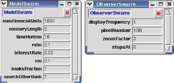
The model depends on the following parameters, illustrated in figure (1): Number of Units = 1000
The number of financial units does not have a strong impact on the outcomes of the simulation, except that financial units must be sufficiently many in order to obtain smooth results. A thousand units are more than strictly necessary and yet not so many to slow down the simulation to problematic times.
Time Horizon = 10
The number of future steps a financial unit looks ahead when considering expected in- and outflows. Similarly to the above case, a very short time horizon would force
*
t
k to take one of a few discrete values. The time horizon should be larger than the
length of memory in order to stress that financial units make their decisions by looking ahead.
Memory Length = 5
The number of past time steps for which financial units remember in- and outflows.
A very short memory, in the order of zero or one, would force kt to take one of a
few discrete values. A memory of five steps is long enough to yield smooth results. Ratio of money outlays to maximum wealth = 0.1
Simulation outcomes are not much affected by the amount of money that is borrowed by financial units unless this is greater than their wealth, in which case all the units go bankrupt very soon. Let us make the more sensible and realistic assumption that financial units borrow a small fraction of the maximum wealth they can own.
Interest Rate = 0.05
The interest rate has little or no effect on the simulation unless it takes unrealistic values such as 50% or higher, in which case all the units go bankrupt very soon. An interest rate of five per cent is a reasonable and innocuous assumption.
Mu = 0.1
Increasing means increasing prudence, which make little sense in a model where loans are granted if just the money to loan is available. Thus, the parameter is meant to be small.
Figure 1
It is clear that most parameters have a negligible effect unless they exceed the boundaries of realism. This is the case of interest rates of 100%, of borrowing sums that exceed wealth by many orders of magnitude, and of very long memories or time horizons.
Thus, we may envisage a wide range of parameter values within which the outcome of the model does not change appreciably. The outcome of the model changes abruptly if the parameters exit this range, but the boundaries of this range coincide with the boundaries of realism so we are not interested in the behaviour of the model outside its range of stability.
The one exception is , the only parameter that influences the simulation in a continuous way. In this case, parameter choice is dictated only by our interest in a system where loans are requested and conceded very easily.
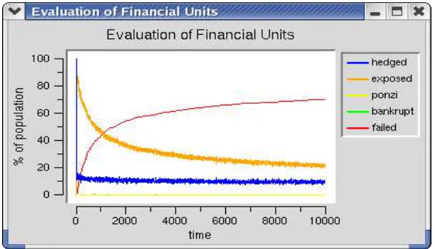
Let us examine the outcomes of the simulation. Figure (2) illustrates the evaluation of financial units according to standard accounting practices after ten thousand steps.
Figure 2
The evaluation of financial units according to standard accounting procedures.
soon as a unit meets the requirements to be classified as “bankrupt”, it fails. In other words, the accounting definition of “bankrupt” is a late predictor of bankruptcy.
Figure (2) shows also that after 10,000 steps about 10% of the financial units are hedged, about 20% are exposed while the remaining 70% went bankrupt. Though most bankruptcies occurred during the first 2,000 steps, the process of going bankrupt never stops. Indeed, by further running the simulation it is possible to see that in about a million steps hedged and exposed units are about 5% each whereas about 90% of the units failed.
Nevertheless, the process of going bankrupt is so slow that during a time lasting hundreds of thousands of steps the economy is composed by a large number of hedged and exposed units. These units lend money to one another according to their evaluation
of ki*,t and ki,t, which may be interesting to observe.
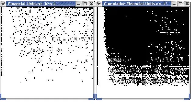
Figure (3) illustrates on the left ki*,t and ki,t on the k* k plane at the 100th
simulation step. Black squares represent pairs of values of ki*,t and ki,t that are taken
by at least one financial unit i at time step t. On the right, figure (3) illustrates the
cumulative occupation of the k* k plane after 100 steps.
Figure 3
Financial units on the k* k plane at the 100th step (left) and cumulative occupation of
The left side of figure (3) makes clear that financial units may evaluate ki*,t and
t i
k, very differently from one another. Within a wide region, the ki*,t and ki,t appear to
be distributed uniformly.
However, this does not happen on the whole of the k* k plane. Indeed, the
salient feature of the right side of figure (3) is that ki*,t and ki,t never take the lowest
values. In fact, low values of ki*,t make a unit concede loans, which worsen
* ,t i
k and,
after some time, ki,t. Units with a high ki,t ask for a loan, and the cycle begins again.
However, this is not a smooth cycle where financial units slowly increase their
* ,t i
k and ki,t. Rather, it is a process of jumps following loan giving and receiving.
Examination of the dynamics of ˆ*
t
k and kˆ confirms this impression. Figures (4)t
and (5) illustrate ˆ*
t
k and kˆ for all units that did not declare bankruptcy for 100 andt
10,000 time steps, respectively.
Figure 4
The indicators ˆ*
t
Figure 5
The indicators ˆ*
t
k and kˆ during the first 10,000 time steps.t
Both ˆ*
t
k and kˆ are subject to irregular endogenous oscillations every few timet
steps. After a transitory, the oscillations of ˆ*
t
k settle in a range that entailed in the upper
part of the range of oscillations of kˆtkˆt, meaning that prospects generally look worse than
they really turn out to be. This is due to the steady flow of units going bankrupt, which for surviving units means that a fraction of the scheduled payments disappear.
The oscillations of ˆ*
t
k and kˆ are not correlated to one another, neither positivelyt
nor negatively. This fact confirms the analysis of the occupation of the k* k, namely,
that no regular dynamics exists.
4. Lenders and Borrowers
What happens if only some financial units are allowed to lend money? Let us run the model with the same parameters as in §3 except that only 10% of the financial units are “banks”. In order to do so, just set banksFraction = 0.1 in the left box of figure (1).
Figure (6) illustrates on the left ki*,t and ki,t at the 10,000th time step. On the
Figure 6
Financial units on the k* k plane at the 100th step (left) and cumulative occupation of
the k* k plane after 100 steps (right), with banksFraction = 0.1.
The notable fact about figure (6) is that the region of the k* k plane that is
actually occupied by financial units is much smaller than in figure (3). Financial units
approach high values of * ,t i
k and ki,t just after going bankrupt. Most of the time, they
stay within a region where * ,t i
k is not too large.
This means that, having specialised some financial units into banking, the expected payment obligations of all units are not allowed to become too bad. Possibly, this is due to the sheer fact that credit has become a scarce resource. Some units are unable to finance their obligations so they go bankrupt rather than making a loan.
Thus, the presence of banks makes the system financially sound, in the sense that financial units are not allowed to reach extremely low levels of liability. This suggests that financial fragility, i.e. the possibility of avalanches of bankruptcies, is more pronounced if banks do not exist or do not work properly.
5. Avalanches of Bankruptcies
all possible lenders, its bankruptcy affects them very little. On the contrary, if a unit that made all of its borrowings from one single other unit goes bankrupt, this lender may have serious problems.
Figure (7) has been obtained by imposing that no lender can be approached besides the one that was chosen at the first simulation step. All parameters as in §3 except that we set searchOtherBank = 0 in the left box of figure (1).
Figure 7
The evaluation of financial units according to standard accounting procedures, with searchOtherBank = 0. Avalanches of bankruptcies become evident.
In figure (7) we can observe that the curve of failed financial units increases stepwise. Each step is an avalanche. We observe one big avalanche of bankruptcies just after the 50th step and a smaller avalanche at about the 65th step.
It is interesting that with preferential lending relations the category “bankrupt units” may become useful in order to predict the onset of an avalanche. In fact, the first big avalanche is preceded by a clear upsurge of the percentage of firms classified as “bankrupt”. However, the category “bankrupt” fails as a predictor so far it regards the second, smaller avalanche.
Figure 8
The evaluation of financial units according to standard accounting procedures, with searchOtherBank = 0 and banksFraction = 0.1. Avalanches are less pronounced.
Coherently with the discussion at the end of §4, we see less and less pronounced avalanches. During the first 100 simulation steps only one avalanche takes place, just after the 50th step as in figure (7). Its size is much smaller than the
corresponding avalanche of figure (7).
Similarly to figure (7), the class of “bankrupt” units is a good predictor of the onset of the avalanche. Further running of the simulation highlights that this is a robust pattern, as shown in figure (9).
Figure 9
6. Conclusions
This contribution had the purpose of highlighting which structural arrangements may make a financial system fragile. Indeed, this is the sort of questions that can be meaningfully asked to an agent-based model. The answer is complementary, not alternative to that provided by models based on differential equations. In fact, where a model based on differential equations may establish that financial fragility exists if certain coefficients are above a certain threshold, an agent-based model may specify under which arrangement that threshold is likely to be reached. This is e.g. the relationships between this contribution and analytical works that make use of the same theoretical framework (Sordi and Vercelli 2003).
Clearly, the framework should be made more realistic if descriptions and predictions on the real world should be made. With firms and banks of different kinds, Governments and international agencies, a lot could be accomplished by means of agent-based models. In principle, plausible financial flows may be reconstructed out of plausible behavioural rules of the agents. Given the secrecy that surrounds this field and the ensuing difficulty to carry out empirical research, agent-based models may find a number of applications.
References
Gilbert N. and Terna P. (2000) How to Build and Use Agent-Based Models in Social Science. Mind & Society, 1: 57-72.
Iori G. and Jafarey S. (2001) Criticality in a Model of Banking Crises. Physica A, 299: 205-212.
Iori G. (2004) An Analysis of Systemic Risk in Alternative Securities Settlement Architectures. European Central Bank Working Paper n. 404.
Iori G., Jafarey S. and Padilla F. (2005) Interbank Lending and Systemic Risk. Journal of Economic Behavior and Organization, forthcoming.
Kindleberger C.P. (1978) Manias, Panics and Crashes: A History of Financial Crises. New York, Basic Books.
Shubik M. (2004) Money and the Monetization of Credit. Working Paper to appear in forthcoming Festschrift, Charles Goodhart.
Sordi S. and Vercelli A. (2003) Financial Fragility and Economic Fluctuations: Numerical simulations and policy implications. University of Siena, Department of Economics, Working Paper n. 407.