Queueing systems to study the energy consumption of a campus WLAN

(1)

Other uses, including reproduction and distribution, or selling or

licensing copies, or posting to personal, institutional or third party

websites are prohibited.

In most cases authors are permitted to post their version of the

article (e.g. in Word or Tex form) to their personal website or

institutional repository. Authors requiring further information

regarding Elsevier’s archiving and manuscript policies are

encouraged to visit:

(2)

Queueing systems to study the energy consumption of a campus

WLAN

Marco Ajmone Marsan

a,b,⇑

, Michela Meo

a

a_{Dipartimento di Elettronica e Telecomunicazioni, Politecnico di Torino, Corso Duca degli Abruzzi 24, 10129 Torino, Italy} b_{IMDEA Networks Institute, Avenida del Mart Mediterraneo, 22, 28918 Leganes (Madrid), Spain}

a r t i c l e i n f o

Keywords:

Energy efﬁciency Wireless LANs Queueing models

a b s t r a c t

In this paper we exploit simple approximate queueing models to assess the effectiveness of the approaches that have been proposed to save energy in dense wireless local area net-works (WLANs), based on the activation of access points (APs) according to the user demand. In particular, we look at a portion of a dense WLAN, where several APs are deployed to provide sufficient capacity to serve a large number of active users during peak traffic hours. To increase capacity, some APs are colocated and provide identical coverage; we say that these APs belong to the samegroup, and they serve users in the same area. The areas covered by different AP groups only partially overlap, so that some active users can only be served by a group of APs, but a fraction of active users can be served by more groups. Due to daily variations of the number of active users accessing the WLAN, some APs can be switched off to save energy when not all the capacity is needed. A real example of this setting is provided by a floor of one building of Politecnico di Torino in Italy, where a student library is located. The approximate analytical models indicate that the energy sav-ing achievable with the proposed approaches is quite substantial, over 40% if at least one AP for each group is always kept on, even with no traffic, to be ready to accept incoming users, and it grows to almost 60% if all APs can be switched off at night, using a separate technology to activate an AP when the first user requests association in the morning.

1. Introduction

It ﬁrst happened to our phones: initially we were accus-tomed to walk to them to answer a call, and to stay there for the entire conversation. We even found it natural not to be reachable while driving. Now, being tied to a cable for just a short call, makes us feel like dogs on leash, and we use our phones when reaching a friend’s home, rather than ringing the door bell. Then it happened to our connec-tions to the Internet: we are now addicted to reading email

wherever we are: on a plane that just landed, in the elevator, in bed, stopping at a red light. . .using our smart-phones, tablets, laptops, phablets, and whatnot. This muta-tion from wired to wireless happened in spite of the unavoidable loss in performance, inherent in the poor characteristics of radio transmission, just because of con-venience. We use our mobile(s) at work, even if the ﬁxed phone is on the desk, and we prefer our laptop(s) to our desktop, even if downloads are slower. To mitigate this performance loss, large organizations have been consis-tently increasing the available bandwidth for mobile data users, by deploying more and more access points (APs) in their wireless local area networks (WLANs). This attitude has led to today’s dense, centrally managed WLANs, where very large numbers of APs are installed, comparable to the

http://dx.doi.org/10.1016/j.comnet.2014.03.012

⇑Corresponding author at: Department of Electronics and Telecom-munications, Politecnico di Torino, Corso Duca degli Abruzzi 24, 10129 Torino, Italy. Tel.: +39 011 0904032.

E-mail address:[email protected](M. Ajmone Marsan).

Contents lists available atScienceDirect

Computer Networks

(3)

maximum number of simultaneously active users (some industrial campuses report over 10 thousand APs).

Even if the individual power consumption of APs is small, the fact that their number is very high implies a remarkable energy consumption and cost (10 W per AP, times 10 thousand APs, times 8760 h in a year, results in 876 MWh a year, with a cost of around 200 thousand euro, using the – admittedly high – kWh price in Italy). Most disturbing is the fact that the majority of this enegy is wasted, since the WLAN capacity that APs provide is not necessary 24/7; rather, capacity should be modulated according to the number of active users, or the trafﬁc they generate, both of which vary widely over hours, days, and weeks; actually, the maximum WLAN capacity is necessary only at peak usage periods, for a limited time.

These considerations, coupled with the growing atten-tion of the networking research community to energy efﬁ-ciency, has led several research groups to investigate the energy saving which is possible with a smart management of WLAN resources, in particular by switching on and off APs according to the required capacity.

The first work in this field is[5], where the authors sug-gest that, in dense WLANs, APs can be clustered, based on their Euclidean distance. When the WLAN traffic (or the number of users) is low, only one AP in each cluster, the cluster-head, is switched on. When the traffic/number of users increases, additional APs can be switched on, to pro-vide adequate capacity. Note that keeping track of the number of users associated with the APs in the cluster is easier (and more stable) than measuring the traffic load, so this quantity is preferred as a control variable in the dense WLAN central controller that turns on/off the cluster APs. The estimated energy saving can be 20–50% in less dense scenarios, whereas in more dense WLANs it can grow to 50–80%. An improvement of the AP clustering scheme was proposed in[6], by using the number and sig-nal strength of the received beacons. This paper also sug-gested that a suitable metric to estimate user demand and drive the provided capacity can be the percentage of time the channel is busy due to transmission and inter-frame spacing.

A similar approach was proposed in[12]to reduce the number of switched-on APs, suggesting that it can be even possible to switch off all the APs in a cluster, provided the area covered by the cluster can be served by neighboring AP clusters. In this case the user demand is estimated from the number of users associated with APs, and energy sav-ings are quantiﬁed in about 60%.

A ﬁrst analytical model for the estimation of the energy gain achievable by modulating the number of switched-on APs as a function of the user demand was proposed in[2], considering just one AP cluster. Assuming as input a mea-sured trafﬁc trace, the analytical predictions indicate that the energy saving can be of the order of 40%.

In [10], the authors developed an ILP (Integer Linear Program) optimization model to adapt the number of switched-on APs to the number and the position of active users, achieving up to 63% power saving. In a subsequent paper [9], the same authors devised a heuristic approach which reduces the problem complexity, but also the achievable power saving.

A WLAN power saving scheme based on the maximum coverage problem was proposed in[3]. The proposed algo-rithm runs on a central controller, which collects the num-ber of users associated with each AP and their data rates, and switches APs on and off dynamically, while maintain-ing coverage and guaranteemaintain-ing user performance. Power saving of about 80% is reported at the expense of frequent user associations and signiﬁcant delays.

The authors of [4]suggest that a drastic reduction of the density of APs in WLANs is possible, provided that the few APs remaining active can provide the coverage required to discover the presence of users. The key point here is that the detection of the user presence is possible with very limited AP coverage, and additional APs can then be switched on, to provide adequate capacity to users. Numerical evaluations show that up to 98% of APs can be switched off with this approach.

Other approaches exist, which are based on the pres-ence of a secondary channel, that can be used to alert switched-off APs of the user presence. For example, the ap-proaches proposed in[13–15]assume that all inactive APs can be switched off regardless of coverage. To react to user presence, an auxiliary low-power channel is available, that wakes the APs when users require access. The authors of

[8]assumed that users are connected to a cellular network, which is capable of requesting the switch-on of a WLAN AP in the vicinity of the user. In[16]the presence of a second-ary Bluetooth interface in both APs and mobile stations is assumed, and the Bluetooth interface can be used to request the activation of the WLAN APs.

In a previous paper [1] we considered a portion of a dense WLAN, where clusters of APs partially overlap in coverage, so that some active users can only be served by the APs of one cluster, but a fraction of active users can be served by APs in more than one cluster. We investigated the energy-performance trade-off with a model based on coupled queues: each queue represents a cluster of colo-cated APs, and customers arriving at the system might be served by one or several queues, depending on their position. We also proposed approximations based on sin-gle-queue and two-queue analysis, which provide fairly accurate performance estimates.

In this paper we expand on those single-queue approx-imate models, ﬁrst showing that measurements of WLAN AP coverage validate the setting we consider, and that measurements of user activity justify the interest in energy saving approaches for a university campus WLAN. Then, we use simple queueing models, with and without setup times, to compare the cases in which the AP wake-up can or cannot exploit the presence of a secondary channel for the detection of user presence.

(4)

little interest was paid in the past to metrics related to en-ergy consumption. This is not due to a limitation in the modeling power of queues; rather, it reﬂects the lack of attention that in the past was paid to the energy character-istics of networks. Now, energy consumption has become an important element of the design space, and models are being developed with the objective of characterizing the energy properties of ICT systems of different types. As a result, energy-related metrics have started to appear in the context of queueing models.

This paper is organized as follows. Section 2contains the problem statement, with the description of the consid-ered portion of the dense WLAN. Section3presents the de-tailed queueing model, together with the considered customer and AP management algorithms. Section 4

describes the approximate queueing model and the computation of performance metrics. Section 5 presents and discusses numerical results obtained with the approx-imate model of the WLAN. Section6presents the variation of the approximate model that includes the AP activation time, and the results which it produces. Section7exploits the model results to quantify the energy saving achievable with the considered AP management scheme. Finally, Section8concludes the paper.

2. Problem statement

In this section, we describe the system we focus on, including the considered customer management (CMN) and AP management algorithms, and we present a detailed queueing model to study the system. For simplicity, we use the case of only two AP clusters in the description, but the extension to more clusters is trivial.

The most important terms of the notation used throughout the paper are summarized inTable 1.

2.1. The wireless LAN

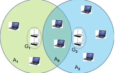
We consider a portion of a dense WLAN in which an area A¼A1[A2is covered by several access points (APs)

in a manner such that a group (we use the term ‘group’ rather than ‘cluster’ because we assume that APs in a group

are colocated, and provide identical coverage, over differ-ent frequency channels; in the literature, clusters deﬁne sets of APs which are not necessarily in the same physical location)G1ofn1APs covers areaA1, and another groupG2

ofn2APs covers areaA2, seeFig. 1for a sketch of the

sys-tem. Each AP can serve up toK mobile terminals (MTs); this means that no more thanKMTs can be associated at the same time with the AP. APs can be switched on and off according to the number of MTs to be served. A fraction

W1 of the total area Acorresponds toA1\A2, so that the

APs in groupG2 cannot serve MTs in this area. Similarly,

a fractionW2of the total areaAcorresponds toA2\A1, that

cannot be served by the APs in group G1. Finally, MTs

located in areaA1\A2¼A0, which corresponds to a

frac-tion 1W1W2¼W0 of the total area, can be served by

any AP. APs can be activated and deactivated based on a given algorithm which is triggered by MT arrivals and departures. When an AP activation is triggered by the arri-val of a MT, the AP switch-on time may translate into an increase of the time needed by the MT to associate with an AP. We will later look at the effect of this time.

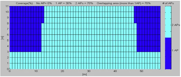
As an example of this setting in a real WLAN, Fig. 2

shows the coverage of one floor of the building of Politec-nico di Torino in which a portion of the main library and some study rooms are located. The top part of the figure re-fers to the estimated signal strength obtained by applying the multiwall model[11]with identical emitted power for the two AP groups; the bottom part of the figure reports di-rect measurements of the actual signal strength, and re-veals that the APs do not actually emit the same power. Assuming a receiver threshold of 70 dBm, the number of AP groups that can be received in the different positions of the floor according to the multiwall model is depicted in

Fig. 3. As can be seen, the coverage areas overlap for a large fraction, about 70% of the total ﬂoor space, meaning that, assuming a uniform distribution of the MTs, only 30% of the MTs need to be served by a speciﬁc AP group and this 30% is evenly divided among the two groups.

MTs are assumed to be uniformly distributed over the area, and to collectively request access according to a Pois-son process with ratek. The MTs remain associated with the AP for a time described by an exponentially distributed random variable with rate

l

. Since the time a MT is associ-ated with an AP depends on the user behavior and only very marginally on the system performance, the rate

l

is

Table 1 Notation.

Symbol Description

ni Number of APs in groupi

K Maximum number of MTs simultaneously associated with an AP

k Rate of association request 1=l Mean association time

Ni Maximum number of MTs associated with groupi ai Probability that a requests is originated from a MT in area

Ai

q System load

g Energy consumption of an active AP [W]

Energy needed for an AP activation/deactivation [J]

ui Number of unconstrained MTs inAi

ci Number of constrained MTs inAi

S State space of the proposed model ci Approximate customer arrival rate toAi 1=d Mean AP switch-on time

A₁

A₂

A₀

G₁

G₂

(5)

independent on the number of MTs in the system. Indeed, the time a MT is associated with an AP is equivalent to the time a user is connected to a network and it is of the order of minutes or hours; thus, the possible effect of network performance on user’s behavior can be considered negligi-ble, and

l

can be made independent on the number of MTs connected to the AP.

As an example of user behavior, we report the analysis of traces collected over the WLAN of Politecnico di Torino, which show quite significant variations over time, that jus-tify the adoption of approaches for the provision of re-sources on demand. Fig. 4 reports the traffic measured during one day in different locations of the Politecnico campus, considering one AP per location type (library, classroom, etc.). Samples are taken every 5 min. The blue line corresponds to the traffic carried by an AP in the area ofFig. 2; the traffic is quite high because this area is contin-uously populated with students that access the study rooms. The pink lowest curve reports the case of an AP lo-cated inside a department, where most of the users have a wired connection and use the WLAN occasionally. The two intermediate curves refer, instead, to an AP in a public area and in a classroom; in both cases the traffic is quite high,

with different behaviors during morning and afternoon, corresponding to the movements of students. Regardless the volume of trafﬁc, the various cases share the same kind of day/night pattern. Similar behaviors can be derived by

Fig. 2.Example of coverage map in a ﬂoor of a Politecnico di Torino building, multi-wall model (top) and measurement (bottom).

Fig. 3.Example of overlapping area in a ﬂoor of a Politecnico di Torino building.

0 20 40 60 80 100 120

01:0002:0003:0004:0005:0006:0007:0008:0009:0010:0011:0012:0013:0014:0015:0016:0017:0018:0019:0020:0021:0022:0023:00

Downloaded Data [MByte]

Classroom Public Area Cafeteria Grnd-Fl

Library Fl-4 Department Fl-3

(6)

observing the number of active MTs. Fig. 5 reports the number of MTs that associate in one hour to anyone of the APs of the main campus in Politecnico (which hosts around 200 APs); the number of generated sessions in one hour is also shown. The day/night behavior is clear and evident, and justiﬁes the use of resource on demand strategies that switch on the APs only when really needed, so that during no trafﬁc periods (such as nights and holi-days) energy can be saved by putting the unneeded APs to sleep.

2.2. The customer management algorithm

In[1]we considered several alternatives as regards the algorithm used to manage unconstrained customers, that correspond to MTs inA0. The considered algorithms differ

in two aspects: (i) the state information that is used to take decisions about MT association with APs: in the various algorithms, state information goes from the simple binary information about the system being full or not, to complete state, including, for all APs, the state and number of associ-ated MTs and (ii) the kind of event that can trigger the algorithm: in some cases the algorithm is triggered by the request of a new MT association, in other cases both arrivals and departures, i.e., MT associations and de-associ-ations, trigger the algorithm.

The results in[1]showed that the more complex algo-rithms bring only small performance improvements with respect to simpler ones, so that the conclusion was that the simplest customer management algorithm could be the wisest choice. In this paper we thus consider only the Random customer management algorithm, according to which each MT in A0 that requests access, chooses the

access point group G1 or G2 with equal probability. If

the chosen group cannot accommodate the MT request, the MT is associated with the other group, if possible. If both groups are full with customers, the request is refused. This algorithm does not explicitly try to optimize energy consumption, allowing MTs to randomly choose the AP group. The only information required at MTs concerns the full/not full state of AP groups at arrival instants.

2.3. The AP management algorithm

The central controller of the dense WLAN collects re-sults about the status of the different components of the WLAN, and in particular of the MT associations to APs, which allow it to control the switch-on and switch-off of APs belonging to different groups, so as to provide re-sources on demand to users, and save energy.

Ideally, a new AP must be switched on when a MT re-quires association to a group of APs where the capacity of the APs which are already on is fully used, and an AP of a group can be switched off when the number of MTs associated with the APs in the group can be handled with one less AP. To switch off an AP it is necessary that the MTs are gathered in the smallest number of APs possible; it is, thus, needed that MTs can hand-off to the desired AP. Since the AP switch-on cannot be instantaneous, but requires switch-on times of the order of 1–2 min, it may be reasonable to introduce a threshold behavior, such that whenjAPs in a group are on, and the total number of MTs associated with them isjKTh, a new AP is switched on.

The threshold Th can be chosen according to the AP

switch-on time, and the association request rate. Similarly, one of the APs can be switched off when the total number of MTs associated with the APs in the group isjKTl, with

Tlpossibly different fromTh, so as to provide a hysteresis

which prevents an excessive frequency of AP switch on/ off events.

3. The detailed queueing model

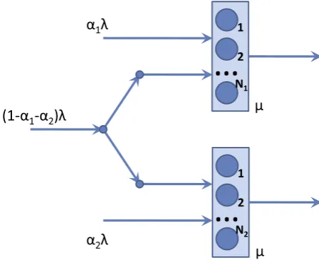
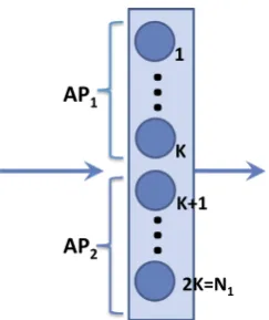
We model the portion of the dense WLAN with the queueing system shown inFig. 6. The queueing system is composed of two multiserver stations with no waiting room. Each station models a group of APs. The service cor-responds to the MT association with an AP. The two sta-tions comprise N1 and N2 servers, respectively, where

Ni¼Knicorresponds to the maximum number of MTs that

can be associated with AP groupi, that is composed ofni

APs, each one limited to host K MTs. As an example,

Fig. 7shows the case of station 1 withn1¼2 APs.

0 400 800 1200 1600 2000 2400 2800

1:00 6:00 11:00 16:00 21:00

# of cards/sessions

hours

Unique cards Sessions

Fig. 5.Example of the number of active MTs (network interface cards) and active sessions measured in an hour in the whole main campus of

(7)

MTs request service, i.e., they request to associate, according to a Poisson process with ratek. This is the cus-tomer arrival process in the queueing model. With proba-bility equal to

a

1an arriving customer is in areaA1\A2and

it is, thus, constrained to proceed to station 1. By assuming uniform arrival rate in the area, the probability to arrive in A1 is proportional to the size of the area, and it is thus

a

1¼W1. If the customer cannot be served by any AP in

group 1, because the maximum number of MTs has already been reached (i.e., it cannot ﬁnd an idle server), the cus-tomer is lost. The same occurs to group 2 with probability

a

2¼W2 (where

a

1þ

a

2<1). With probability

a

0¼W0¼

1

a

1

a

2, an arriving customer is unconstrained, i.e., it

can be associated with either one of the two groups, according to the system CMN algorithm, and the customer is lost only when no idle server exists at either station. As an example, for the case presented in Figs. 2 and 3, in which 70% of the area is common, and the remaining is evenly distributed among the two groups, the model parameter setting corresponds to

a

1¼

a

2¼0:15.

Service times are i.i.d. random variables with exponen-tial distribution with rate

l

. The system load can be de-ﬁned as

q

¼k=

l

.

Each AP (and the correspondingKservers in the model) can be eitheractiveorinactive. Active servers can be either busy, i.e., serving a customer, or idle, i.e., ready to provide service to an incoming customer. In the model, the transi-tion of an AP from inactive to active and vice versa corre-sponds to groups ofKservers that, at a time, become idle or active. We assume that as soon asKactive servers are idle, their corresponding AP is deactivated, and that if all active servers are busy when a customer arrives,Kinactive servers (one inactive AP) are activated, if available. This implies settingTh¼Tl¼0.

We assume that each active AP (group of K servers) consumes energy at a rate

g

W, while an inactive AP (a group of K inactive servers) consumes negligible energy. The energy consumption may be a function of load, or of the number of active servers in the group; however, in this paper we always assume

g

to be constant, which is consis-tent with the characteristics of today’s hardware. The acti-vation or deactiacti-vation of an AP requires an energy equal to

J.

The state of the queueing system is deﬁned by a qua-druple s¼ ðu1;c1;u2;c2Þ, with ui the number of

uncon-strained customers at station i and ci the number of

constrained customers at station i. Considering that uiþci6Ni, the cardinality of the state spaceSis given by:

jSj¼ ðN1þ1ÞðN1þ2Þ

2

ðN2þ1ÞðN2þ2Þ

2

ð1Þ

that is of the order ofðN1N2Þ 2

.

4. The approximate queueing model

As we can see from(1), the cardinality of the state space Sof the queueing system grows roughly with the fourth power of the maximum number of users that can be served by a group of APs (assuming that the two groups can serve about the same number of users). If the number of AP groups is n, and each group can serve at most N users, the state space cardinality is of the order ofN2n_{. This means}

that the Markovian model that underlies the queueing sys-tem suffers from a combinatorial explosion of the number of states for both growing number of users and growing number of AP groups.

In order to tackle the problem of very large state spaces, in [1] we introduced approximate models that provide accurate estimates of the performance metrics, while gen-erating state spaces of much smaller size than the detailed model discussed so far, and even allowing in some case a closed form expression for the limiting probabilities.

The simplest approximation is based on considering just one of the two queues in our system, say queue 1. The idea behind this approach is to approximate the customer arri-val rate

c

1at queue 1 from the areaA0¼A1\A2,

indepen-dently of the state of the other queue (queue 2). The performance metrics of interest are then computed for queue 1, independently from the state of queue 2.

The customer arrival rate inA0 is equal to

a

0k.

Accord-ing to the Random CMN algorithm, this rate is equally split between the two queues, so that queue 1 receives from this area a customer ﬂow at rate

a

0k=2. However, queue 1 also

receives all customers that arrive in areaA0when queue 2

is full, so that we must also account for an additional cus-tomer arrival rate equal to P½f2a0k=2, where P½f2 is the

probability that queue 2 is full. So, we can write:

c

1¼ ð1þP½f2Þ

a

0k

2 ð2Þ

The total arrival rate at queue 1 is then:

k1¼

a

1kþ ð1þP½f2Þ

a

0k

2 ð3Þ

Assuming that the two queues are equal (same number of APs, same size of the served area, same maximum num-ber of users per AP), or very similar, we can approximate the value ofP½f2with the valueP½f1. If the parameters of

the two queues are indeed identical, we only introduce an error deriving from the fact that we are assuming inde-pendence in the behavior of the two queues. If the param-eters of the two queues differ, an additional error is introduced by assumingP½f2 ¼P½f1.

For the model solution, in this case we must use an iter-ative algorithm, because of the circular dependence of the loss probability on the arrival rate, and of the arrival rate

(8)

on the loss probability. At each step of the iteration, the probability distribution vector ~

p

is computed, as well as P½f1, for a given value of the customer arrival ratek1. The

new value of k1 is then computed from P½f1, and a new

iteration is run. The algorithm stops when either a maxi-mum number of iterations is reached, or the relative error between the values ofP½f1at two consecutive steps of the

iteration is smaller than a given tolerance. The perfor-mance measures of interest are computed from the ﬁnal probability distribution vector.

Note that the queue we are using in this approximation is anM=M=N1=0, with arrival rate equal to k1, so that the

state space cardinality is simply N1þ1, and the limiting

probabilities can be expressed in closed form as:

p

i;1¼

k1

l

i 1 i!

PN1

k¼0

k1

l

k 1 k!

ð4Þ

fori¼0;. . .;N1, and

P½f1 ¼

p

N1;1 ð5Þ

Hence, the iterative algorithm is extremely fast.

Note that the limiting distribution for this queue is invariant with respect to the service time distribution.

This approach can be easily extended to cases compris-ing more than two queues.

In [1] we validated this approximate model, and we showed that it can be quite accurate for symmetrical set-tings, like the one presented inFig. 3. We also presented and validated other, more complex approximations, based on several separate queues, which are better suited to asymmetrical cases.

In what follows, we will report only the results obtained with the simplest approximation, in which one queue is used to model a group of APs. We will denote bykthe over-all arrival rate at the queue, by

l

the customer service rates and by

p

i the probability that there areicustomers in the

queue, i.e., thatiMTs are associated with the group of APs. Moreover,Nwill be the maximum number of MTs that can associate with a group that is composed ofnAPs, so that

N¼nK.

4.1. The performance metrics

For the WLAN and the queueing system we introduce the following performance metrics:

average number of customers at each station (average number of MTs associated with the AP group),

averageutilizationof the APs,

averagepower consumptionof the APs,

averageenergy consumed to serve one customer,

average and cumulative distribution function (CDF) of

the active time of an AP, i.e., the time between the

instant in which an AP is switched on and when it is switched off again.

Whenicustomers are in the station, the amount of MTs associated with APxof the group is given by:

cxðiÞ ¼

0 for i6_ðx1_ÞK

nmodK for ðx1ÞK <i<xK

K for iPxK

8 > < >

: ð6Þ

The average number of customers at APxcan then be computed as:

E½Nx ¼

XN

i¼1

cxðiÞ

p

i ð7Þ

The average utilization of APxcan be computed by:

E½Ux ¼

XN

i¼ðx1ÞKþ1

p

i ð8Þ

The average power consumption can be computed as:

E½P ¼E½Ps þE½Pact þE½Pde ð9Þ

where E½Ps is the power consumed by active APs, and

E½Pact;E½Pde are the powers consumed for server group

activation and deactivation, respectively. We have:

E½Ps ¼

g

XN

i¼1

di=Ke

p

i ð10Þ

where the term in the sum represents the number of active APs.

The power to activate and deactivate an AP is given by the product of the energy needed to activate and deacti-vate an AP multiplied by the frequency with which this happens. Thus:

E½Pact ¼

k

Xn1

x¼0

p

xK ð11Þ

E½Pde ¼

l

Xn1

x¼0

xKþ1

ð Þ

p

xKþ1 ð12Þ

since in statexKthe arrival of a customer with ratekcauses the activation of APxþ1, and in statexKþ1 the departure of a customer, event that occurs with rateðxKþ1Þ

l

, causes the switch off of APx.

The average energy consumed to serve one customer can be computed as:

E½Ec ¼

E½PE½T

E½N ¼

E½P

kð1P½lossÞ ð13Þ

whereE½Tis the average time spent by a customer in the queueing system, which is computed by Little’s Law as:

E½T ¼ E½N

kð1P½lossÞ with E½N ¼

XN

i¼1

ipi ð14Þ

The AP active time can be computed from the ﬁrst pas-sage time between the states in which activation and deac-tivation can occur.

5. Numerical results

(9)

power and of the AP active times so as to derive insight into the effectiveness of using AP activation and deactiva-tion as a way to reduce energy consumpdeactiva-tion.

We consider the case of 3 APs per group, with the maximum number of associated MTs per AP, K¼8. We set the time that each MT remains associated with an AP to be exponentially distributed with mean equal to 10 min, and we varyk. The load is denoted by

q

¼k=

l

. In what follows, we call AP1 the ﬁrst AP to be switched on, i.e., the one which handles the ﬁrstKMTs associated with APs in the group, AP2 the second AP to be switched on, i.e., the one which handles theKMTs in excess of theKhandled by AP1, and AP3 the one that handles the MTs that are associated with the group in excess of 2K.

The energy consumption per time unit for each access point is assumed to be constant, and is set to

g

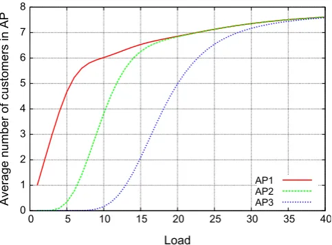
¼10 W. The energy spent for an AP activation or deactivation is ne-glected, i.e., we set

¼0 J.

Fig. 8shows the average number of MTs associated with the three APs versus the load of the AP group. As expected, the average number of MTs associated with AP1 is larger than for AP2, which in turn is larger than for AP3. The num-ber of MTs associated with AP2 is negligible for load less than 3, and the number of MTs associated with AP3 is neg-ligible for load less than 8. Considering meaningful loads to be lower than 24 (the number of servers) we see that the maximum average utilizations of APs are around 7 for AP1 and AP2, and around 6 for AP3, for a total of about 20 MTs in the AP group on average.

Fig. 9 shows the average utilization of AP1, AP2, and AP3, as deﬁned before, as well as the curve of the AP group being idle (no MT associated with any AP). If the APs in the group behave ideally, i.e., if they can be acti-vated and deactiacti-vated in zero time according to the num-ber of MT associations (no active AP if no MT is associated with APs in the group, 1 active AP if the number of asso-ciated MTs is between 1 and K, 2 active APs between Kþ1 and 2K, and 3 active APs beyond 2K), then the aver-age number of active APs for each load value is given by the sum of the values of the three AP curves, and the power consumption in W is obtained by just applying a factor

g

.

Fig. 10reports the average active time for the three APs versus the AP group load. Clearly, when the load is low, say below 6, one active AP is sufﬁcient: the number of associ-ated MTs is usually smaller thanK¼8, and it is very unli-kely that the second AP (AP2) switches on. In case this happens, the time that AP2 remains active is very small. When the load grows, say between 6 and 20, the typical number of associated MTs is larger than 8, so that AP1 is almost always on (this translates in extremely long active times) and AP2 is on for increasingly long periods, while AP3 switches on rarely, and when this happens it remains active for very short times only. For even higher values of the AP group load (up to 40) AP3 exhibits increasingly long active times, up to about 2 h.

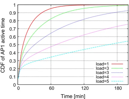
The CDF of the active time of AP1 is shown inFig. 11for different (but low) values of the AP group load. The CDF re-ﬂects the behavior observed above. For example, when the load is very low, equal to 1, 95% of the times that AP1 switches on, it remains active for less than 1 h. When the load is higher, for example equal to 5, the active time is much longer, and only 35% of the times it is shorter than 1 h. In most cases, the probability that the active time of AP1 is shorter than 5 min is less than 20%. The fact that, even for very low loads, the probability of short active times is small, makes the AP switch-on times (that we

0 1 2 3 4 5 6 7 8

0 5 10 15 20 25 30 35 40

Average number of customers in AP

Load

AP1 AP2 AP3

Fig. 8.Average number of MTs associated with each AP versus load.

0 0.1 0.2 0.3 0.4 0.5 0.6 0.7 0.8 0.9 1

0 5 10 15 20 25 30 35 40

AP utilization

Load

AP1 AP2 AP3 idle

Fig. 9.Average AP utilization versus load.

0 100 200 300 400 500 600

0 5 10 15 20 25 30 35 40

AP active time [min]

Load

AP1 AP2 AP3

(10)

observed in experimental setups to be of the order of 1–2 min) largely irrelevant for the overall system performance.

Nevertheless, in the next section we modify our approx-imate model to account for the switch-on time of AP1.

6. Model with AP1 activation time

The model that we have presented in the previous sec-tions is based on the assumption that an AP can be switched on or off instantaneously, according to the num-ber of MTs that associate with the AP group. This assump-tion is justified by the large ratio between AP active times and switch on/off times, as well as the possibility of intro-ducing thresholds to anticipate the activation of APs when the capacity of the active APs is close to exhaustion. In this section we nevertheless investigate the impact of the switch-on time of AP1, assuming that all the APs that cover a given area are switched off in periods of no traffic. This implies the existence of a secondary method for the iden-tification of user presence, so that AP1 is switched on for example in the morning when the first student entering the study room switches on her/his PC.

This amounts to modifying the queueing model dis-cussed in the previous sections by introducing a delay be-tween the arrival of the customer that finds an empty queue, and the beginning of service. If the delay can be as-sumed to be exponentially distributed, with rated, the con-tinuous-time Markov chain (CTMC) model underlying the queueing system requires that in the state definition, in addition to recording the number of associated MTs, mem-ory is kept about the state of AP1 (active or not). Let the state be given by the pair of values ði;sÞ, where i is the number of customers in the system and s2 f0;1g repre-sents the service being available (s¼1 means AP1 active) or unavailable (s¼0 means AP1 inactive). When the queue is empty, at the arrival of the first customer, the CTMC moves to stateð1;0Þin which AP1 is being activated and the customer is waiting for service. Further arrivals can oc-cur during the activation period, with no service in pro-gress. When AP1 finally activates, if there areicustomers waiting, the CTMC moves with rate d from ði;0Þ to ði;1Þ

and services start. The state space cardinality is equal to 2Nþ1, where N is the maximum number of MTs that can be associated with the AP group.

It is also possible to assume a constant switch-on time (which can be more realistic). In this case, the queueing model can no longer be described with a CTMC, but the semi-Markov process underlying the queueing model can still be analyzed by using an embedded discrete-time Mar-kov chain (DTMC). In the embedded chain, the idle state represents the cases in which no service is in progress. The exit from the DTMC idle state corresponds to the AP1 activation, and occurs after the arrival of the ﬁrst MT fol-lowed by the constant activation time; out of the idle state the DTMC moves towards any possible active state, depending on the number of arrivals that occurred during the activation time. In this case, the state space of the DTMC comprisesNþ1 states.

The results that we discuss next refer to the case in which the AP activation time is either exponentially dis-tributed, with average comprised between 0.5 and 2 min, or constant, with the same range of values.

Fig. 12shows curves of the probability that a user has to wait that AP1 switches on, versus the AP group traffic load, for values of the average switch-on time that very between 30 s and 2 min. For the same cases,Fig. 13shows the aver-age time that a user has to wait. We can see that the prob-ability that a user has to wait that AP1 switches on is almost invariant with respect to the average switch-on time, and that the probability is high only for very low traffic values. We also note that the average time that a user has to wait is less than 10 s for all traffic load values larger than 3.

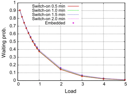
The next two ﬁgures,Figs. 14and15, compare the cases of exponentially distributed and constant AP switch-on times. The waiting probabilities computed using the two models are almost identical, while the average waiting times are slightly shorter in the (more realistic) case of constant switch-on times, as expected.

7. Energy saving

In this section we exploit the approximate models presented in this paper to assess the effectiveness of AP 0

0.1 0.2 0.3 0.4 0.5 0.6 0.7 0.8 0.9 1

0 60 120 180

CDF of AP1 active time

Time [min]

load=1 load=3 load=3 load=4 load=5

Fig. 11. Cumulative distribution of the active time of AP1 under various values of the load.

0 0.1 0.2 0.3 0.4 0.5 0.6 0.7 0.8 0.9 1

0 1 2 3 4 5

Waiting prob.

Load Switch-on 0.5 min Switch-on 1.0 min Switch-on 1.5 min Switch-on 2.0 min

(11)

management schemes by focusing on the achievable reduction in AP energy consumption. In order to consider

a realistic setting, we take as input a daily trafﬁc pattern obtained from the one reported inFig. 4, scaling it down to be representative of the considered area, which com-prises two groups of APs with 3 APs each. In particular, we assume that, at the peak hour, the trafﬁc load is

q

¼N. For each value of the hourly load we derive the stea-dy-state solution of the approximate model (with no AP activation time) and we compute the energy consumption of the AP group in three cases: (i) the 3 APs are always on; (ii) one AP is always on to be ready to serve MTs entering the area, and the other two are turned on only when necessary; and (iii) all APs can be switched off when no MT requests service in the considered area, since a second-ary method is available to detect the arrival of MTs requesting association.

Fig. 16shows the average energy consumption of each one of the 3 APs for each hour, under the considered daily trafﬁc pattern. We can see that no energy is necessary dur-ing the night, since no MT is present in the area covered by the AP group, and that the periods of activity are different for the 3 APs.

The results inFig. 16can be combined to generate the total energy consumption of the AP group in the three 0

0.2 0.4 0.6 0.8 1 1.2 1.4 1.6 1.8 2

0 1 2 3 4 5

Waiting time [min]

Load Switch-on 0.5 min Switch-on 1.0 min Switch-on 1.5 min Switch-on 2.0 min

Fig. 13. Average time that a user has to wait that AP1 switches on, versus the AP group load, for variable average switch-on time.

0 0.1 0.2 0.3 0.4 0.5 0.6 0.7 0.8 0.9 1

0 1 2 3 4 5

Waiting prob.

Load Switch-on 0.5 min Switch-on 1.0 min Switch-on 1.5 min Switch-on 2.0 min Embedded

Fig. 14.Model with AP activation time, comparison between the CTMC and embedded MC model: average time that a user has to wait that AP1 switches on versus load.

0 0.2 0.4 0.6 0.8 1 1.2 1.4 1.6 1.8 2

0 1 2 3 4 5

Waiting time [min]

Load Switch-on 0.5 min Switch-on 1.0 min Switch-on 1.5 min Switch-on 2.0 min Embedded

Fig. 15.Model with AP activation time, comparison between the MC and embedded MC model: average time that a user has to wait that AP1 switches on versus load.

0 2 4 6 8 10 12

0 5 10 15 20

Average consumption [W]

Time [h] AP1

AP2 AP3

(12)

cases. We see inFig. 17that if we assume that the 3 APs are always on, the AP group power consumption is constant, equal to 30 W. If instead AP1 is always on, but the other two APs are turned on only when necessary, the power consumption is 10 W from 7 pm to 7 am, and is following the daily trafﬁc pattern in the other half of the day. Finally, if all APs can be switched off when no MT requests service in the considered area, no power is consumed by the AP group from midnight to 6 am, and the power consumption is proportional to trafﬁc for the rest of the day.

If we integrate the power consumption to compute the energy absorbed from the grid, which translates into cost for the network operator, we see that if we assume that the 3 APs are always on, the total daily energy consump-tion is equal to 0.72 kWh (about 263 kWh a year). If AP1 is always on, and the other two APs are turned on only when necessary, the total daily energy consumption is equal to 0.41 kWh. If all APs can be switched off when no MT requests service in the considered area, the total daily energy consumption is equal to 0.31 kWh. This implies a saving of 43% if AP1 is always on, and of 57% if AP1 is switched off in the periods of no trafﬁc. It should be noted that the increased saving comes at a cost, since it requires

the existence of a technology (possibly a secondary – low power – radio channel) to detect the presence of users requesting association when no AP is active.

Finally, inFig. 18we show, for the same setting, the fre-quency at which APs switch on during each hour of the day. We see that AP1 switches on only when trafﬁc is very low: in the early morning and late evening. AP2 switches on later in the morning and earlier in the evening. AP3 instead switches on (and off) during most of the day, fol-lowing the ﬂuctuations in the number of users that request association in the considered area. By looking at the integral of the switch-on rate, we can conclude that the average number of switch-on/off for AP1 is lowest, and the one for AP3 is highest.

8. Conclusions

Sleep modes for APs are being studied by several re-search teams as a promising approach to improve the en-ergy efficiency of WLANs. They can be specially effective in dense centrally-managed WLANs, where a large number of APs is deployed to provide high capacity, which is how-ever necessary only at peak times, for a short portion of the day. In this paper, we presented simple queueing models to assess the effectiveness of AP sleep modes in dense WLANs, using the setting of one floor of the Politecnico di Torino campus as an example. We computed several dif-ferent performance and energy parameters, showing that the energy saving achievable with the proposed ap-proaches is quite substantial, of the order of 43% if at least one AP for each group always remains on, even with no traffic, to be ready to accept incoming users, and it grows to about 57% if all APs can be switched off at night, thanks to a separate technology to activate an AP when the first user requests association in the morning.

The main insight provided by our analysis is the follow-ing. First, we proved that the energy saving potential is quite substantial: more than half of the energy used to power on a campus WLAN can be saved. Second, we showed that the impact of AP switch-on/off times is negli-gible, since typical on and off periods are much longer (at least one order of magnitude on average, for reasonable traffic load) than the transient duration. Third, we showed that the added benefit of a secondary technology to wake up sleeping APs, thanks to which all APs can be switched off during long periods of no traffic (specially night) is important (almost 15% of the total energy).

Finally, we showed that, even in new networking sce-narios, queueing models[7]remain a simple and effective tool for the investigation of the system behavior and for the selection of the most beneﬁcial operating modes.

Acknowledgements

The research leading to these results has received fund-ing from the EU 7th Framework Programme (FP7/2007-2013) under Grant Agreement n. 257740 (NoE TREND).

We would like to thank Christian Tipantuna for the work on the coverage maps and propagation models; Fikru 0

5 10 15 20 25 30 35 40

0 5 10 15 20

Average consumption [W]

Time [h] All dynamic APs

AP1 always on no AP management

Fig. 17. Average total consumption in a typical day, with and without coverage continuity.

0 0.02 0.04 0.06 0.08 0.1 0.12 0.14 0.16 0.18

0 5 10 15 20

Frequency [min

-1]

Time [h]

AP1 AP2 AP3

(13)

Getachew, Nanfang Li, Marco Ricca and Yi Zhang for pro-viding the plots with measurement results.

References

[1]Marco Ajmone Marsan, Ana Paula Couto da Silva, Michela Meo,

Energy-performance trade-off in dense WLANs: a queuing study,

Elsevier Comput. Networks 56 (11) (2012) 2522–2537.

[2] Marco Ajmone Marsan, Luca Chiaraviglio, Delia Ciullo, Michela Meo, A simple analytical model for the energy-efﬁcient activation of access points in dense WLANs, in: 1st International Conference on Energy-Efﬁcient Computing and Networking, June 2010, pp. 159–168.

[3] Kwan-Wu Chin, A green scheduler for enterprise WLANs, in: Australasian Telecommunication Networks and Applications Conference (ATNAC ’11), 2011, pp. 1–3.

[4] Fatemeh Ganji, Lukasz Budzisz, Adam Wolisz, Assessment of the Power Saving Potential in Dense Enterprise WLANs, Technical Report TKN-13-003, TKN Group, TU Berlin, April 2013.

[5] Amit P. Jardosh, Gianluca Iannaccone, Konstantina Papagiannaki, Bapi Vinnakota, Towards an energy-star WLAN infrastructure, in: 8th IEEE Workshop on Mobile Computing Systems and Applications (HotMobile ’07), March 2007, pp. 85–90.

[6]Amit P. Jardosh, Konstantina Papagiannaki, Elizabeth M. Belding,

Kevin C. Almeroth, Gianluca Iannaccone, Bapi Vinnakota, Green WLANs: on-demand WLAN infrastructures, Mobile Networks Appl.

14 (6) (2009) 798–814.

[7]Leonard Kleinrock, Queueing Systems: Volume I – Theory, Wiley

Interscience, New York, 1975.

[8]SuKyoung Lee, SungHoon Seo, Nada Golmie, An efﬁcient

power-saving mechanism for integration of WLAN and cellular networks,

IEEE Commun. Lett. 9 (12) (2005) 1052–1054.

[9] Josip Lorincz, Massimo Bogarelli, Antonio Capone, Dinko Begusic, Heuristic approach for optimized energy savings in wireless access networks, in: International Conference on Software, Telecommunications and Computer Networks (SoftCOM ’10), 2010, pp. 60–65.

[10] Josip Lorincz, Antonio Capone, Massimo Bogarelli, Energy savings in wireless access networks through optimized network management, in: 5th International Symposium on Wireless Pervasive Computing (ISWPC ’10), May 2010, pp. 449–454.

[11] Ingo Forkel, Matthias Lott, A multi wall and ﬂoor model for indoor radio propagation, in: IEEE Vehicular Technology Conference (VTC 2001-Spring), May 2001.

[12] Riichiro Nagareda, Akio Hasegawa, Tatsuo Shibata, Sadao Obana, A proposal of power saving scheme for wireless access networks with access point sharing, in: International Conference on Computing, Networking and Communications (ICNC ’12), 2012, pp. 1128–1132. [13] Suhua Tang, Hiroyuki Yomo, Yoshihisa Kondo, Sadao Obana, Exploiting burst transmission and partial correlation for reliable wake-up signaling in Radio-On-Demand WLANs, in: IEEE International Conference on Communications (ICC ’12), 2012, pp. 4954–4959.

[14] Suhua Tang, Hiroyuki Yomo, Yoshihisa Kondo, Sadao Obana,

Wake-up receiver for radio-on-demand wireless LANs, EURASIP J. Wireless

Commun. Network. 2012 (1) (2012) 1–13.

[15] Hiroyuki Yomo, Yoshihisa Kondo, Kosuke Namba, Suhua Tang, Takatoshi Kimura, Tetsuya Ito, Wake-up ID and protocol design for radio-on-demand wireless LAN, in: IEEE 23rd International

Symposium on Personal Indoor and Mobile Radio Communications (PIMRC ’12), 2012, pp. 419–424.

[16]Jong-Woon Yoo, Kyu Ho Park, A cooperative clustering protocol for

energy saving of mobile devices with WLAN and Bluetooth

interfaces, IEEE Trans. Mobile Comput. 10 (5) (2011) 491–504.

Marco Ajmone Marsan holds a double appointment as Full Professor at the Depart-ment of Electronics and Telecommunications of the Politecnico di Torino (Italy), and Research Professor at IMDEA Networks Insti-tute (Spain).

He earned his graduate degree in Electrical Engineering from the Politecnico di Torino in 1974 and completed his M.Sc. in Electrical Engineering at the University of California at Los Angeles (USA) in 1978. In 2002, he was awarded a ‘‘Honoris Causa’’ Ph.D. in Tele-communication Networks from the Budapest University of Technology and Economics.

From 2003 to 2009 he was Director of the IEIIT-CNR (Institute for Elec-tronics, Information and Telecommunication Engineering of the National Research Council of Italy). From 2005 to 2009 he was Vice-Rector for Research, Innovation and Technology Transfer at Politecnico di Torino. He is involved in several national and international scientiﬁc groups: He was Chair of the Italian Group of Telecommunication Professors (GTTI); the Italian Delegate in the ICT Committee and in the ERC Committee of the EC’s 7th Framework Programme. He is a Fellow of the IEEE and he is listed by Thomson-ISI amongst the highly-cited researchers in Computer Science.

He has been principle investigator for a large number of research con-tracts with industries, and coordinator of several national and interna-tional research projects.