Partial inversion of the elliptic operator to speed up computation of likelihood in Bayesian inference

Partial inversion of the elliptic operator to speed up

computation of likelihood in Bayesian inference

Alexander Litvinenko

August 6, 2020

Contents

1 Introduction 2

1.1 Main idea . . . 5

1.2 Bayesian updating formula . . . 6

2 Hierarchical domain decomposition (HDD) method 8 2.1 Notation . . . 10

2.2 Mapping Φω = (Φgω,Φfω) . . . 12

2.3 Mapping Ψω = (Ψgω,Ψfω) . . . 12

2.4 Φω and Ψω in terms of the Schur complement matrix . . . 13

3 Construction Process 13 3.1 Initialisation of the recursion . . . 14

3.2 Recursion . . . 14

3.3 Building of Matrices Ψω and Φω from Ψω1 and Ψω2 . . . 17

3.4 Algorithms “Leaves to Root” and “Root to Leaves” . . . 18

3.5 Multiple scales . . . 19

4 Hierarchical matrix approximation 19 5 Fast Evaluation of Functionals 19 5.1 Computing the mean value in all subdomains ω ∈TTh . . . 21

5.2 Algorithms for computing the mean values . . . 23

5.3 Solution in a subdomain . . . 24

6 Numerics 25

7 Conclusion and discussion 27

A Appendix A 35

†_{E-mail: [email protected]. RWTH Aachen, Aachen, Germany}

1

Abstract

Often, when solving forward, inverse or data assimilation problems, only a part of the solution is needed. As a model, we consider the stationary diffusion problem. We demonstrate an algorithm that can compute only a part or a functional of the solu-tion, without calculating the full inversion operator and the complete solution. It is a well-known fact about partial differential equations that the solution at each discreti-sation point depends on the solutions at all other discretidiscreti-sation points. Therefore, it is impossible to compute the solution only at one point, without calculating the solu-tion at all other points. The standard numerical methods like a conjugate gradient or Gauss elimination compute the whole solution and/or the complete inverse operator. We suggest a method which can compute the solution of the given partial differential equation 1) at a point; 2) at few points; 3) on an interface; or a functional of the solution, without computing the solution at all points. The required storage cost and computational resources will be lower as in the standard approach.

With this new method, we can speed up, for instance, computation of the innovation in filtering or the likelihood distribution, which measures the data misfit (mismatch). Further, we can speed up the solution of the regression, Bayesian inversion, data as-similation, and Kalman filter update problems.

Applying additionally the hierarchical matrix approximation, we reduce the cubic

computational cost to almost linear O(k2nlog2n), wherek n and nis the number

of degrees of freedom.

Up to the hierarchical matrix approximation error, the computed solution is exact. One of the disadvantages of this method is the need to modify the existing deterministic solver.

Keywords: mismatch, innovation, data misfit, likelihood, Bayesian inversion, Bayesian formula, partial inverse, FEM, domain decomposition, hierarchical matrices, H-matrices, elliptic problem, data-sparse H-matrix approximation, multiscale

AMS 65F10, 60H15, 60H35, 65C30

1

Introduction

We further develop the method, initially introduced in [31, 22, 7, 32] and in Chapter 12 of [21]. With this method, we will be able to compute the solution in a subdomain, in a point, the mean value over a subdomain and other functionals F(u) without computing the full inverse operator and the complete solution. Similar ideas were considered in [1, 39]. This method can be very practical for speeding up the solution of the inverse and data assimilation problems, which appear in many science and engineering applications such as weather prediction, oil recovery, and subsurface flow. Under the inverse problem, we understand the estimation of unknown model parameters from (noisy) measurements. Under the data assimilation problem, we understand improving the existing mathematical model when the new measurement data become available.

Table 0.1: Notation

HDD suggested here the hierarchical domain decomposition method

u|γ restriction of the solution uonto the interface γ

h, H grid step sizes on fine and coarse meshes Ω, ∂Ω computational domain and its boundary

Z random parameter vector Z = (Z1, ..., ZnZ)

Θ space where parameterZ = (Z1, ..., Znz) is defined

ω, ∂ω local subdomain and its boundary

Vh, VH two finite element spaces,VH ⊂Vh

f, fh, fH the right hand side, discretized on fine (h) and coarse (H) meshes u,uh,uH the solution, computed on fine (h) and coarse (H) meshes

κ(x, Z) =eq(x,Z) _{uncertain permeability coefficient, depends on parameter vector Z}

VN vector space spanned on the basis {ϕ1(x), . . . , ϕN(x)}

I,IN index sets

Th, TH fine and coarse triangulations

TTh hierarchical domain decomposition tree

γω interface in the domainω ⊂Ω (also call “internal” boundary) Γω =∂ω boundary (also call “external” boundary)

dω dω :=

(fi)_i∈I(ω),(gi)i∈I(∂ω)

= (fω, gω)

a composed vector consisting of the right-hand side restricted toω

and the Dirichlet boundary values gω =uh|∂ω Fh, Gh two operators, such that uh =Fhfh +Ghgh,

ˆ

y true observations

y= ˆy+ε noisy observations Φg

ω :RI(∂ω)→RI(γω) maps the boundary data defined on ∂ω to the data defined on the interface γω

Φf

ω :RI(ω) →RI(γω) maps the right-hand side data defined onω to the data defined on γω.

Ψf_ω :_RI(ω) →_RI(∂ω) _{maps the whole subdomain to the external boundary}

Ψg

ω :RI(∂ω)→RI(∂ω) maps the external boundary to the external boundary pdf probability density function

The Bayesian inference is a statistical inference method in which Bayes’ theorem is used to update the probability for a hypothesis as more evidence or information becomes available. Computing the likelihood function in the Bayesian formula requires multiple solutions of the forward problem and could be time-consuming. Depending on the available measure-ments, the complete solution of the (forward) diffusion problem could be unnecessary, rather only a part of the solution or a functional of the solution is needed. Computing only a part of the solution will make the whole computing process faster and less time-consuming.

Typically, the available measurement data is a functionalF(u) of the solutionu. The mis-fit (or mismatch) function is the difference between the simulated data and the measurement values [58, 56, 45, 46, 53, 57]. Below we will show how to simulate these measurement data directly without computing the whole solution. Particularly, we will show that calculating the full inverse operator is unnecessary.

One possible application of our method is the data driven research, a very popular topic nowadays. In this research the available datasets are used either to improve (enrich) the existing mathematical model (often a system of PDEs), or to discover the governing system of PDEs. Another example when fast calculation of a part of the solution is required, is computing the mean square error when comparing the training and computed datasets. In [55], authors design data-driven algorithms for inferring solutions to various partial differen-tial equations. They introduce neural networks that are trained to solve supervised learning tasks while respecting any given laws of physics described by general nonlinear PDEs. Their goal is to solve two classes of problems: data-driven solution and data-driven discovery of PDEs.

The structure of this paper is the following. In Section 1 we give our motivation by intro-ducing the stochastic forward problem and the Bayesian updating procedure for computing posterior density function of the uncertain diffusion coefficient. The main ingredient and the main contribution — the hierarchical domain decomposition (HDD) method — is contained in Section 2. Details of the HDD method, including two algorithms “Leaves to Root” and “Root to Leaves”, are shown in Section 3. The hierarchical (denoted by H) - matrix tech-nique to speed up the HDD method is explained in Section 4. Section 5 explains how to use the HDD method to compute a functional of the solution without computing the whole solution. Particularly, it explains how to compute the mean value in a small subdomain. The novelty here is that the whole solution is not available, only a small part of it. In the last section, we conclude the main achievements.

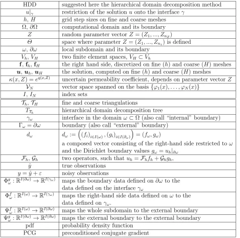
Example. This example shows how the solution (or measurements) in only a few points can reduce the uncertainty. Consider an elliptic PDE with uncertain coefficient and the right hand side as in Eq. 1.1, but in 1D, on the interval [0,1]. We pose uncertain Dirichlet boundary conditions g(0, ξ) and g(1, ξ), where ξ is a Gaussian random variable. Assume three measurements at locations x={0.3,0.5,0.8}are given. The mean valuesu(0.3) = 22,

u(0.5) = 28, u(0.8) = 18 and the standard deviations are {0.2,0.3,0.3} respectively. The following computations are done with the stochastic Galerkin library sglib, written by E. Zander at TU Braunschweig 1. In Fig. 1.1 twenty realisations of the uncertain solutionu(x) before and after an update are shown. The mean value (dark bold line) and±{1,2,3} stan-dard deviations (red, orange and yellow lines) are shown. The left picture shows realisations, obtained with some prior assumption about distribution of random diffusion coefficient κ.

In the following three pictures of the updated solutions are shown, after taking into account one, two and three measurements. To conclude this example, it is practical to have a nu-merical method, which can efficiently compute a part of the solution or a solution in a few points, without computing the complete solution.

0 0.5 1

-20 0 20 40 60

0 0.5 1

-20 0 20 40 60

0 0.5 1

-20 0 20 40 60

0 0.5 1

-20 0 20 40 60

Figure 1.1: (left) 20 original realisations of the solutionu(2nd, 3rd, 4th) the same realisations after update; the mean value (bold line) and ±1,2,3 standard deviations (red, orange and yellow lines).

1.1

Main idea

The main ingredients of the developed approach are the weak formulation, the hierarchical (or recursive) domain decomposition technique, the finite element method, and the Schur complement. Additionally, to speed up matrix operations and reduce the overall storage cost, we approximate the involved operators and the Schur complement in the hierarchical matrix format [20, 17, 21].

The noveltyof this work is the application of the HDD method for faster computation of the innovation in filtering or the likelihood distribution, which measures the data misfit (mismatch).

The forward problem we consider is an elliptic boundary value problem with uncertain

L∞ coefficients and with Dirichlet boundary condition:

−∇(κ(x, Z)∇u(x, Z)) =f(x), x∈Ω⊂_R2_,

u=g(x), x∈∂Ω, (1.1)

where κ(x, Z) is a random field dependent on a random parameterZ = (Z1, ..., Znz)∈R

nz_,

nz ≥ 1, consisting of a set of independent continuous random variables characterizing the random coefficient of the governing equation. The solution u(x, Z) is a stochastic quantity, given by

u(x, Z) : Ω×_Rnz _→

Rn, (1.2)

where n is the number of finite element nodes in Ω.

For a fixed Z, the solution u(x, Z) belongs to H1(Ω), and for a fixed x toL2(Θ). There

the uniqueness and the existence of the solution. Additionally, they offer a new method with weaker assumptions. If the expansion of κ is truncated, there is no guaranteed that the truncated series will stay strictly bounded from zero. As a result, the existence of the approximate solution to Eq. 1.1 is questionable, unless precautions are taken as in [43]. The settings where the ellipticity condition is preserved are considered in [11].

Further we assume that each continuous random variable Zi has a prior distribution

Fi(zi) =P(Zi ≤zi)∈[0,1], (1.3) where P denotes probability and πi(zi) = dF_dzi(zi)

i probability density function (pdf). The

joint prior density function for Z is πZ(z) =

Qnz

i=1πi(zi). For the sake of simplicity, we will skip the subscript Z and will write π(z) for denoting the probability density function of the random variable Z.

The elliptic boundary value problem in Eq. 1.1, can represent, for instance, an incom-pressible single-phase porous media flow or, another example, a steady state heat conduction through a composite material. In the single-phase flow, u is the flow potential, and κ the permeability of the porous medium. For heat conduction in composite materials, u is the temperature, −κ∇u the heat flow density, and κ the thermal conductivity.

Iterative methods and preconditioners to solve the problem in Eq. 1.1 were developed in [27, 28, 44, 59, 64]. In [10] the authors assume that the solution has a low-rank canonical (CP) tensor format and develop methods for the CP-formatted postprocessing.

Tensor ranks of the stochastic operator were analysed in [47, 9]. The proper generalized decomposition was applied for solving high dimensional stochastic problems in [51, 52]. In [26] authors employed newer tensor formats for the approximation of coefficients and the solution of stochastic elliptic PDEs. Other classical techniques to cope with high-dimensional problems are sparse grids [18, 4, 50] and (quasi) Monte Carlo methods [15, 63, 29]. In [6, 5] authors approximate the polynomial chaos expansion (PCE ) of the random input coefficient

κ(x, Z) in the tensor train (TT) data format, and then solve the problem in that format. A low-rank tensor approximation of random fields, covariance matrices and set of snapshots is done in [25, 37, 35].

1.2

Bayesian updating formula

The inverse problem and propagation of uncertainty through a computational (forward) model are strongly connected. Prior and posterior probabilities express our belief about possible values of the parametersκ(x, Z) before and after observations.

Various ideas to speed up the Bayesian updating procedure were presented in [42, 40, 49, 3]. Surrogate based techniques were presented in [56, 47, 34]; reduction of the stochastic dimension by using KLE and PCE expansions in [58, 53, 56]; a non-linear Kalman filter extension in [46, 45, 36].

Further we assume that Θ is a measure space with σ-algebra A and with a probability measure _P, and thatq :Θ → Q and u: Θ → U are random variables (RVs). Often, we are not able to observe the entityq ∈ Qdirectly, we can only see a ‘shadow’ of it, formally given by a ‘measurement operator’

Y :Q × U 3 (q, u)7→Y(q;u)∈ Y, (1.4) where q(x, Z) = log(κ(x, Z)). We assume that the space of possible measurements Y is a vector space, which frequently can be regarded as finite-dimensional, as one can only observe a finite number of quantities.

The measurement operator Y with values in Y produces

y(Z) =Y(q(Z);u), where u=u(q(Z)).

Examples of measurements are a) y(Z) = R_ωu(Z, x)dx, with a subdomain ω ⊂ Ω, and b)

u in a few points. For a given f, the measurement y is just a function of q. This function is usually not invertible since the measurement y does not contain enough information. In the Bayesian framework, the state of knowledge is modeled in a probabilistic way. The parameter q is uncertain and is modeled by a random variable. The Bayesian setting allows updating/sharpening of information about q when the measurement is performed.

Usually the observation of the “truth” ˆy ∈ _Rny _{will deviate from what we expect to}

observe even if we know the right q due to some model error . The measurement can be also polluted by some measurement error ε. Hence we observe y = ˆy++ε, and would like to know what q is. Let S : _Rnz _→

Rny be the solution operator (for instance, the set

{Φg_,Φf_{}or the inverse) of Eq. 1.1. For the sake of simplicity we will only consider one error} term

y= ˆy+ε =S(Z) +ε, where ε= (ε1, ..., εny)∈R

ny _{includes all the errors. (1.5)}

Hereε1, ..., εny are mutually independent random variables with probability density function

π(ε) =Qny

i=1π(εi). We also assume here that ε and Z are independent.

The mapping in Eq. (1.4) is usually not invertible, and hence the problem is called ill-posed. By modeling our lack of knowledge about q in a Bayesian way [62] with a Q-valued random variable, the problem becomes well-posed [61]. But of course one is looking now at the problem of finding a probability distribution that best fits the data; and one also obtains a probability distribution of q. Here we focus on the use of Bayesian approach [14].

Bayes’s theorem is commonly accepted as a consistent way to incorporate new knowledge into a probabilistic description. It may be formulated as ([62] Ch. 1.5)

π(z|y) = R π(y|z)

Θπ(y|z)πz(z)dz

πz(z), (1.6)

where πz(z) is the pdf of Z, π(y|z) is the likelihood as a function of y for fixed prior Z and

π(z|y) is the posterior pdf of Z conditioned on the data y. We follow the notation from [41]. Numerical approaches for computing a posterior pdf were developed in [40, 42, 61, 56]. Assuming independence on the measurement noiseε = (ε1, . . . , εny), the likelihood function

becomes

L(z) :=π(y|z) = ny

Y

i=1

Again, we see a formula, where the noisy measurement yi should be compared with the computed simulationSi(z). And very often, the complete solution is not required.

2

Hierarchical domain decomposition (HDD) method

The hierarchical domain decomposition (HDD) method [31] combines the weak formulation, the finite element method (FEM), and the recursive domain decomposition method to obtain a fast and efficient algorithm for computing the partial inverse and a part of the solution (without computing the complete solution). This method was introduced by Hackbusch in 2002 and later on developed in [31, 32, 22, 7, 21].

HDD computes the solution operatorsFh and Gh in Eq. 2.2, which after applying to the boundary condition and the right-hand side give us the solution.

Below in this section we define the main components of the HDD method - the hierarchical domain decomposition tree (see Fig. 2.2) in Section 2.1, the boundary-to-boundary mappings (Ψg) in Section 2.3, domain-to-boundary (Ψf) mappings in Section 2.2, boundary-to-interface (Φg_{) and domain-to-interface (Φ}f_{) mappings which are essential for the definition of the HDD} method in Section 2.2.

For a fixed parameter Z, Eq. 1.1 can be written as follow:

−∇(κ(x)∇u(x)) =f(x), x∈Ω⊂_R2_{, (2.1)}

u=g(x), x∈∂Ω,

where x= (x1, x2)∈Ω.

The HDD method computes two discrete hierarchical solution operators Fh and Gh such that:

uh =Fhfh+Ghgh, (2.2)

where uh = uh(fh, gh) is the FE solution of 2.1, fh the discretized right-hand side, and gh the Dirichlet boundary data. To decrease the computing time and the storage cost, both operators Fh and Gh are approximated by H-matrices.

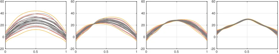
Figure 2.1: (a) The solution u|γ on the interface γ can be computed with the auxiliary operator Φ, by applying it to the right hand side f and to the boundary conditionu|∂Ω; (b)

HDD can compute the solution in a subdomain ω ⊂ Ω; (c) HDD method can compute the solution on a coarse mesh (shown by dotted lines).

1. Suppose the solution on the boundary ∂Ω (Fig. 2.1 (a)) is given. One is interested in the fast numerical approach which computes the solution u|γ on the interface γ. The solution u|γ depends on the right-hand side and u|∂Ω = g, i.e. u|γ = Φ(u|∂Ω, f) with

some mapping Φ;

2. Only the solution in a small subdomain ω ⊂ Ω is of interest (Fig. 2.1 (b)). To solve the problem in a domain ω the boundary values on ∂ω are required. How to compute them efficiently from the global boundary data ∂Ω and the given right-hand side?

3. The third possible problem setup is as follows. The solution on the interface or on a very coarse mesh (see Fig. 2.1 (c)) is required. How can this solution be computed effectively without neglecting small scale features?

Other properties of the HDD method are the following. The HDD allows one to compute

uh(fh, gh) for fh given in a smaller space VH ⊂ Vh. This could be useful, for instance, in multi-scale settings. The HDD provides the possibility to computeuh restricted to a coarser grid with reduced computational effort. The HDD shows big advantages in complexity for problems with multiple right-hand sides and multiple Dirichlet data. In this case both operators Fh and Gh are computed only once and then applied multiple times to fh and gh. Due to the binary tree structure the HDD is an easily parallelizable method. If the problem contains repeated patterns (for instance, so-called cells in a multi-scale framework) then the computational resources can be reduced drastically.

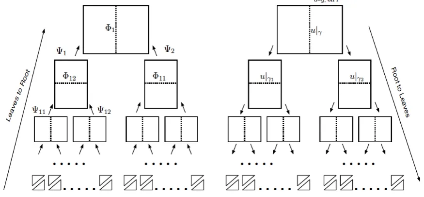
Figure 2.2: HDD contains two algorithms: “Leaves to Root” (shown on the left) which computes mappings {Ψ1,Ψ2,Ψ11,Ψ12, . . .} and {Φ1,Φ2,Φ11,Φ12, . . .} and “Root to Leaves”

(on the right) which applies mappings{Φij} to compute the solutions u|γi on the interfaces

2.1

Notation

LetTh be a triangulation of the spatial domain Ω. After hierarchical decomposition of Ω (cf. [12]), obtain thehierarchical domain decomposition tree TTh (see Fig. 2.2) with the following

properties:

• Ω is the root of the tree, • TTh is a binary tree,

• Ifω ∈TTh has two sons ω1, ω2 ∈TTh, then

ω=ω1∪ω2 and ω1, ω2 have no interior point in common,

• ω∈TTh is a leaf, if and only ifω ∈ Th.

The construction of TTh is straight-forward by dividing Ω recursively into subdomains. For

practical purposes, the subdomains ω1, ω2 must both be of size ≈ |ω|/2 and the internal

boundary

γω :=∂ω1\∂ω =∂ω2\∂ω (2.3)

must not be too large (see Fig. 3.1 (left)).

1 2

3 4 5 6

8 7

9 10 11 12

inner boundary

extern boundary

Figure 2.3: Domain ω1 ∈TTh with I(ω1) ={1, ...,12}, I(∂ω1) ={3,4,5,6,7,8,9,10,11,12},

I(γω1) = {1,2} to be eliminated via the Schur complement, I(Γω1) = {9,7,3,4,5,6,8,12}.

On the next level, when ω1 will be coupled with ω2, the points I(γω) = {10,11} will be eliminated.

Let I := I(Ω) and xi, i ∈ I, be the set of all nodal points in Ω (including nodal points on the boundary). We define I(ω) as a subset of I with xi ∈ ω = ω. Similarly, we define

I(ω◦), I(Γω), I(γω), where Γω :=∂ω, ◦

ω =ω\∂ω, for the interior, for the external boundary and for the interface.

Computing the discrete solution uh, Eq. 1.1, in Ω is equivalent to the computation of uh on all γω, ω ∈ TTh, since I(Ω) =∪ω∈TT_hI(γω). These computations are performed by using the linear mappings Φf_ω, Φg_ω defined for all nodes ω ∈TTh.

Notation 2.1 Let gω := u|I(∂ω) be the local Dirichlet data and fω := f|I(ω) be the local

Definition 2.1 The mapping Φg

ω : RI(∂ω) → RI(γω) maps the boundary data defined on ∂ω to the data defined on the interface γω. Φfω : RI(ω) → RI(γω) maps the right-hand side data defined on ω to the data defined on γω.

The final aim is to compute the solution uh along γω in the form uh|γω = Φ

f

ωfω + Φgωgω,

ω ∈ TTh. For this purpose HDD builds the mappings Φω := (Φ

g

ω,Φfω), for all ω ∈ TTh.

For computing the mapping Φω, ω ∈ TTh, we first need to compute the auxiliary mapping

Ψω := (Ψgω,Ψfω) which will be defined later.

Thus, the HDD method consists of two steps: the first step is the construction of the mappings Φg

ω and Φfω for all ω ∈ TTh. The second step is the recursive computation of the

solutionuh. In the second step HDD applies the mappings Φgω and Φfω to the local Dirichlet data gω and to the local right-hand side fω.

Notation 2.2 Let ω∈TTh and

dω :=

(fi)_i∈I(ω),(gi)i∈I(∂ω)

= (fω, gω) (2.4)

be a composed vector consisting of the right-hand side from Eq. 1.1 restricted to ω and the Dirichlet boundary values gω =uh|∂ω (see also Notation 2.1).

Note that gω coincides with the global Dirichlet data in Eq. 1.1 only when ω = Ω. For all other ω ∈ TTh we compute gω in (Eq. 2.4) by the algorithm “Root to Leaves” (see Section

3.4).

Assuming that the elliptic boundary value problem, Eq. 2.1, restricted toωis solvable, we can define the local FE solution by solving the following discrete problem in the variational form [19]:

(

aω(Uω, bj) = (fω, bj)_L2_(ω), ∀j ∈I(

◦

ω), Uω(xj) =gj, ∀j ∈I(∂ω).

(2.5)

Here, bj is the P1-Lagrange basis function atxj andaω(·,·) is the bilinear form (see Eq. 1.1) with integration restricted to ω and (fω, bj) =

R

ω

fωbjdx.

Let Uω ∈ Vh be the solution of (Eq. 2.5) in ω. The solution Uω depends on the Dirichlet data on∂ω and the right-hand side in ω. Dividing problem (Eq. 2.5) into two subproblems (Eq. 2.6) and (Eq. 2.7), we obtain Uω =Uωf +Uωg, whereUωf is the solution of

(

aω(Uωf, bj) = (fω, bj)_L2_(ω), ∀j ∈I(

◦

ω), U_ωf(xj) = 0, ∀j ∈I(∂ω)

(2.6)

and Ug

ω is the solution of

aω(Uωg, bj) = 0, ∀j ∈I( ◦

ω), Ug

ω(xj) =gj, ∀j ∈I(∂ω).

(2.7)

2.2

Mapping

Φ

= (Φ

,

Φ

)

In this section we define mappings Φω, Φgω, Φfω. We consider ω ∈ TTh with two sons ω1, ω2.

Considering once more the datadω from (Eq. 2.4),Uωf from (Eq. 2.6) andUωg from (Eq. 2.7), we define Φf

ω(fω) and Φgω(gω) by Φf_ω(fω)

i :=U f

ω(xi) ∀i∈I(γω) (2.8) and

(Φg_ω(gω))_i :=Uωg(xi) ∀i∈I(γω). (2.9) Since Uω =Uωf +Uωg, we obtain

(Φω(dω))_i := Φωg(gω) + Φfω(fω) =Uωf(xi) +Uωg(xi) =Uω(xi) (2.10)

for all i∈I(γω).

Hence, Φω(dω) is the trace ofUω onγω. Definition in (Eq. 2.10) says that if the datadω are given then Φω computes the solution of (Eq. 2.5). Indeed, Φωdω = Φggω + Φffω. Note that the solution uh of the initial global problem coincide with Uω inω, i.e., uh|ω =Uω.

2.3

Mapping

Ψ

= (Ψ

,

Ψ

)

In this section we define mappings Ψω, Ψgω, Ψfω. First, we define the mapping Ψf_ω from (Eq. 2.6) as

Ψf ω(dω)

i∈I(∂ω) :=aω(U

f

ω, bi)−(fω, bi)_L2_(ω), (2.11)

where U_ωf ∈Vh, Uωf|∂ω = 0 and

a(U_ωf, bi)−(f, bi) = 0, for ∀i∈I( ◦

ω).

Second, we define the mapping Ψg

ω from (Eq. 2.7) by setting (Ψg

ω(dω))i∈I(∂ω) :=aω(Uωg, bi)−(fω, bi)L2_(ω) =aω(Uωg, bi)−0 =aω(Uωg, bi), (2.12) where U_ωg ∈Vh and (Ψgω(dω))i = 0 for ∀i∈I(

◦

ω).

The linear mapping Ψω, which maps the datadω given by (Eq. 2.4) to the boundary data on∂ω, is given in the component form as

Ψω(dω) = (Ψω(dω))i∈I(∂ω) :=aω(Uω, bi)−(fω, bi)L2_(ω). (2.13)

By definition Ψω is linear in (fω, gω) and can be written as Ψω(dω) = Ψfωfω+ Ψgωgω. Here

Uω is the solution of the local problem (Eq. 2.5) and it coincides with the global solution on

2.4

Φ

and

Ψ

in terms of the Schur complement matrix

Let the linear systemAu=Fcforω∈TTh be given. In Sections 3.1 and 3.3 we explain how

to obtain the matricesA andF. Ais the stiffness matrix for the domain ω after elimination of the unknowns corresponding toI(ω◦\γω). The matrixF comes from the applied numerical integration rule [31].

We will write for simplicity γ instead of γω. Thus, A : RI(∂ω∪γ) → RI(∂ω∪γ), u ∈ RI(∂ω∪γ), F : RI(ω) → RI(∂ω∪γ) and c ∈ RI(ω). Decomposing the unknown vector u into

two components u1 ∈RI(∂ω) and u2 ∈RI(γ), obtain

u=

u1

u2

.

The component u1 corresponds to the boundary ∂ω and the component u2 to the interface

γ. Then the equation Au=Fc becomes

A11 A12

A21 A22

u1

u2

=

F1

F2

c, (2.14)

where

A11 :RI(∂ω)→RI(∂ω), A12 :RI(γ) →RI(∂ω),

A21:RI(∂ω) →RI(γ), A22 :RI(γ) →RI(γ),

F1 :RI(ω)→RI(∂ω), F2 :RI(ω) →RI(γ).

The elimination of the internal points is done as it is shown in (Eq. 2.15) below

A11−A12A−221A21 0

A21 A22

u1

u2

=

F1−A12A−221F2

F2

c. (2.15)

We rewrite the last system as two equations ˜

Au1 := (A11−A12A−221A21)u1 = (F1−A12A−221F2)c,

u2 =A−221F2c−A−221A21u1.

(2.16)

The explicit expressions for the mappings Ψω and Φω follow from (Eq. 2.16):

Ψg_ω :=A11−A12A−221A21, Ψfω :=F1−A12A−221F2, (2.17)

Φg_ω :=−A₂₂−1A21, Φfω :=A −1

22F2. (2.18)

Thus,u2 = Φfω(fω) + Φgω(gω), with the rhs fω =c, and local b.c. gω =u1.

3

Construction Process

In this section we explain the recursive construction of mappings Ψg

3.1

Initialisation of the recursion

This section explains how to compute mapping Ψf_ω for the leaves of TTh and how it is

connected with the quadrature rule.

Our purpose is to get for each triangle ω ∈ Th, the system of linear equations

A·u= ˜c:=F ·c, (3.1)

where A is the stiffness matrix, c the discrete values of the right-hand side in the nodes of

ω and F will be defined later. The matrix coefficients Aij are computed by the formula

Aij =

Z

ω

κ(x)h∇bi(x)· ∇bj(x)idx, (3.2)

where bi(x) is a piecewise linear basis function [19]. For ω ∈ Th, F ∈ R3×3 comes from the discrete integration and the matrix coefficients Fij are computed using (Eq. 3.5). The components of ˜ccan be computed as follows:

˜

ci =

Z

ω

f bidx≈

f(x1)bi(x1) +f(x2)bi(x2) +f(x3)bi(x3)

3 · |ω|, (3.3)

where xi, i ∈ {1,2,3}, are three vertices of the triangle ω ∈ TTh, bi(xj) = 1 if i = j and

bi(xj) = 0 otherwise. Rewrite (Eq. 3.3) in matrix form:

˜ c=   ˜ c1 ˜ c2 ˜ c3  ≈ 1 3  

b1(x1) b1(x2) b1(x3)

b2(x1) b2(x2) b2(x3)

b3(x1) b3(x2) b3(x3)



 



f(x1)

f(x2)

f(x3)



, (3.4)

where f(xi), i = 1,2,3, are the values of the right-hand side f in the vertices of ω. Then, for piecewise linear basis functions obtain

F := 1 3





b1(x1) b1(x2) b1(x3)

b2(x1) b2(x2) b2(x3)

b3(x1) b3(x2) b3(x3)

 = 1 3  

1 0 0 0 1 0 0 0 1



 and c:=





f(x1)

f(x2)

f(x3)



. (3.5)

Thus, Ψg_ω corresponds to the matrix A∈_R3×3 _{and Ψ}f

ω toF ∈R3×3.

3.2

Recursion

This section explains how to build Ψω from Ψω1 and Ψω2, with ω ∈ TTh and ω1, ω2 be two

sons ofω. The coefficients of Ψω can be computed by (Eq. 2.13). The external boundary Γω of ω splits into (see Fig. 3.1 (left))

Γω,1 :=∂ω∩ω1, Γω,2 :=∂ω∩ω2. (3.6)

For simplicity of further notations, we will writeγ instead of γω.

Suppose that by induction, the mappings Ψω1, Ψω2 are known for the sons ω1, ω2. Now, we

explain how to construct Ψω and Φω.

Lemma 3.1 Let the data d1 =dω1, d2 =dω2 be given by (Eq. 2.4). Data d1 and d2 coincide

along γω, i.e.,

• (consistency conditions for the boundary)

g1,i=g2,i ∀i∈I(ω1)∩I(ω2), (3.7)

• (consistency conditions for the right-hand side)

f1,i=f2,i ∀i∈I(ω1)∩I(ω2). (3.8)

If the local FE solutions uh,1 and uh,2 of the problem (2.5) for the data d1, d2 satisfy the

additional equation

γ_Ψ

ω1(d1) +

γ_Ψ

ω2(d2) = 0, (3.9)

then the composed solution uh defined by assembling

uh(xi) =

uh,1(xi) for i∈I(ω1),

uh,2(xi) for i∈I(ω2)

(3.10)

satisfies (Eq. 2.5) for the data dω = (f, g) where

fi =

f1,i for i∈I(ω1),

f2,i for i∈I(ω2),

(3.11)

gi =

g1,i for i∈I(Γω,1),

g2,i for i∈I(Γω,2).

(3.12)

Proof: Note that the index sets in (Eq. 3.10)-(Eq. 3.12) overlap. Let ω1 ∈ TTh, f1,i = fi,

i∈ I(ω1), and g1,i =gi, i∈ I(∂ω1). Then the existence of the unique solutions of (Eq. 2.5)

gives uh,1(xi) =uh(xi),∀i∈I( ◦

ω1).

In a similar manner we get uh,2(xi) = uh(xi) , ∀i∈I( ◦

ω2). Equation (Eq. 2.13) gives

(γΨω1(d1))i∈I(γ) =aω1(uh, bi)−(fω1, bi)L2_(ω

1) (3.13)

and

( γΨω2(d2))i∈I(γ) =aω2(uh, bi)−(fω2, bi)L2_(ω

2). (3.14)

The sum of the two last equations (see Figure 3.1 (right)) and (Eq. 3.9) give

0 = γΨω(dω)i∈I(γ) =aω(uh, bi)−(fω, bi)L2_(ω). (3.15)

We see that uh satisfies (Eq. 2.5).

Note that

uh,1(xi) =g1,i =g2,i =uh,2(xi) holds for i∈I(ω1)∩I(ω2).

Next, we use the decomposition of the data d1 into the components

Figure 3.1: (left) Domain ω and its two sons ω1 and ω2. Here γω is the internal boundary and Γω,i, i = 1,2, parts of the external boundaries, see (Eq. 3.6). (right) The support of basis function bj, xj ∈ω1 and xj ∈ω2.

where

g1,Γ := (g1)i∈I(Γω,1), g1,γ := (g1)i∈I(γ) (3.17)

and similarly for d2 = (f2, g2,Γ, g2,γ). The decomposition g ∈_RI(∂ωj) _intog

j,Γ ∈RI(Γω,j) and gj,γ ∈RI(γ) implies the decomposition of Ψg_ωj : _RI(∂ωj) _→

RI(∂ωj) into ΨΓωj : R

I(Γω,j) _→

RI(∂ωj) and Ψγωj :R

I(γ) _→

RI(∂ωj), j = 1,2.

Thus, Ψg

ω1gω1 = Ψ

Γ

ω1g1,Γ+ Ψ

γ

ω1g1,γ and Ψ

g

ω2gω2 = Ψ

Γ

ω2g2,Γ+ Ψ

γ ω2g2,γ.

The maps Ψω1, Ψω2 become

Ψω1d1 = Ψ

f

ω1f1+ Ψ

Γ

ω1g1,Γ+ Ψ

γ

ω1g1,γ, (3.18)

Ψω2d2 = Ψ

f

ω2f2+ Ψ

Γ

ω2g2,Γ+ Ψ

γ

ω2g2,γ. (3.19)

Definition 3.1 We will denote the restriction of Ψγ ωj :R

I(γ) _→

RI(∂ωj) _{to I(γ) by}

γ_Ψγ ωj :R

I(γ) _→

RI(γ),

where j = 1,2 and ∂ωj = Γω,j∪γ.

Restricting (Eq. 3.18), (Eq. 3.19) to I(γ), we obtain from (Eq. 3.9) and g1,γ = g2,γ =: gγ that

γ_Ψγ ω1 +

γ_Ψγ ω2

gγ = (−Ψfω1f1−Ψ

Γ

ω1g1,Γ−Ψ

f

ω2f2−Ψ

Γ

ω2g2,Γ)|I(γ).

Next, we set M :=−( γ_Ψγ ω1 +

γ_Ψγ

ω2). and after computing M

−1_{, we obtain:}

gγ =M−1(Ψfω1f1+ Ψ

Γ

ω1g1,Γ+ Ψ

f

ω2f2+ Ψ

Γ

ω2g2,Γ)|I(γ). (3.20)

Remark 3.1 The inverse matrixM−1 _{exists since it is the sum of positive definite matrices}

corresponding to the mappings γΨγ_ω1, γΨγ_ω2.

Remark 3.3 We have the formula Ψω(dω) = Ψω1(d1) + Ψω2(d2), where

dω = (fω, gω), d1 = (f1, g1,Γ, g1,γ), d2 = (f2, g2,Γ, g2,γ),

g1,γ =g2,γ =M−1(Ψfω1f1 + Ψ

Γ

ω1g1,Γ+ Ψ

f

ω2f2+ Ψ

Γ

ω2g2,Γ)|I(γ).

(3.21)

Here (fω, gω) is build as in (Eq. 3.11)-(Eq. 3.12) and (Eq. 3.7),(Eq. 3.8) are satisfied.

Conclusion:

Thus, using the given mappings Ψω1, Ψω2, defined on the sons ω1, ω2 ∈TTh, we can compute

Φω and Ψω for the father ω∈TTh.

3.3

Building of Matrices

Ψ

and

Φ

from

Ψ

and

Ψ

Let ω, ω1 where ω2 ∈TTh and ω1, ω2 are sons ofω. Recall that ∂ωi = Γω,i∪γ. Suppose we

have two linear systems of equations forω1 and ω2 which can be written in the block-matrix

form:

A(₁₁i) A(₁₂i) A(₂₁i) A(₂₂i)

!

u(₁i) u(₂i)

!

= F

(i)

11 F

(i) 12

F₂₁(i) F₂₂(i)

!

c(₁i) c(₂i)

!

, i= 1,2, (3.22)

where γ :=γω,

A(₁₁i) :_RI(Γω,i)_→

RI(Γω,i), A(12i):R

I(γ)_→

RI(Γω,i),

A(₂₁i):_RI(Γω,i) _→

RI(γ), A(22i):R

I(γ)_→

RI(γ),

F₁₁(i) :_RI(ωi\γ) _→

RI(∂ωi), F12(i):RI(γ)→RI(∂ωi),

F₂₁(i) :_RI(ωi\γ) _→

RI(γ), F22(i):R

I(γ)_→

RI(γ).

Both the equations in (Eq. 3.22) are analogous to (Eq. 3.18) and (Eq. 3.19). Note that c(1)₂ =c(2)₂ and u(1)₂ =u(2)₂ because of the consistency conditions (see (Eq. 3.7),(Eq. 3.8)) on the interfaceγ. The system of linear equations for ω be



 

A(1)₁₁ 0 A(1)₁₂

0 A(2)₁₁ A(2)₁₂ A(1)₂₁ A(2)₂₁ A(1)₂₂ +A(2)₂₂

     

u(1)₁ u(2)₁ u(1)₂

  =   

F₁₁(1) 0 F₁₂(1)

0 F₁₁(2) F₁₂(2) F₂₁(1) F₂₁(2) F₂₂(1)+F₂₂(2)

     

c(1)₁ c(2)₁ c(1)₂





. (3.23)

See the left matrix in Fig. A.1 in the Appendix. Using the notation

˜

A11:=

A(1)₁₁ 0 0 A(2)₁₁

!

, A˜12:=

A(1)₁₂ A(2)₁₂

!

,

˜

A21:= (A (1)

21, A

(2)

21), A˜22 :=A

(1)

22 +A

(2)

22,

˜

u1 :=

u(1)₁ u(2)₁

!

, u˜2 :=u (1)

2 =u

(2)

2 ,

˜

F1 :=

F₁₁(1) 0 F₁₂(1)

0 F₁₁(2) F₁₂(2)

!

, F˜2 :=

F₂₁(1), F₂₁(2), F₂₂(1)+F₂₂(2)

˜ c1 :=

c(1)₁ c(2)₁

!

, ˜c2 :=c (1)

2 =c

(2)

2 , ˜c:=

˜ c1

˜ c2

,

the system (Eq. 3.23) can be rewritten as

˜

A(₁₁i) A˜(₁₂i)

˜

A(₂₁i) A˜(₂₂i)

!

˜

u1

˜

u2

=

_˜

F1

˜

F2

˜

c. (3.24)

The system (Eq. 3.24), indeed, coincides with (Eq. 2.14). After elimination of variablesu(2)₁

(on the interface), we obtain the matrices as it shown in Figures 4.1 and 4.2.

3.4

Algorithms “Leaves to Root” and “Root to Leaves”

The scheme of the recursive process of computing Ψω and Φω from Ψω1 and Ψω2 for all ω ∈TTh is shown in Fig. 2.2 (left). We call this process “Leaves to Root”:

1. Compute Ψf ω ∈R3

×3 _{and Ψ}g ω ∈R3

×3 _{on all leaves of T}

Th (triangles of Th) by (Eq. 3.2)

and (Eq. 3.5).

2. Compute recursive from leaves to root Φω and Ψω from Ψω1,Ψω2. Store Φω and delete

Ψω1,Ψω2.

3. Stop if ω = Ω.

Remark 3.4 The result of this algorithm will be a collection of mappings {Φω : ω ∈ TTh}.

The mappings Ψω, ω ∈TTh, are only of auxiliary purpose and need not stored.

The algorithm which applies the mappings Φω = (Φgω,Φfω) to compute the solution we call “Root to Leaves”. This algorithm starts from the root and ends on the leaves. Figure 2.2 (right) presents the scheme of this algorithm.

Let the data dω = (fω, gω), ω = Ω, be given. We can then compute the solution uh of the initial problem as follows.

The Algorithm “Root to Leaves”:

1. Start with ω= Ω.

2. Given dω = (fω, gω), compute the solution uh on the interior boundaryγω by Φω(dω).

3. Build the data dω1 = (fω1, gω1), dω2 = (fω2, gω2) from dω = (fω, gω) and gγω := Φω(dω).

4. Repeat the same for the sons of ω1 and ω2.

5. End if ω does not contain internal nodes.

Since uh(xi) =gγ,i, the set of values (gγω), for all ω ∈TTh, results the solution of the initial

3.5

Multiple scales

Let h and H be fine and coarse meshes, used for discretization of Eq. 2.1. The subscript h near the operator or function means that this operator or function was discretized on a mesh with the step size h. Let nh and nH be the numbers of degrees of freedom on a fine grid and on a coarse grid. For instance, if the right-hand side is smooth, we may use a coarser mesh for it (e.g., operatorFH andGh). So, the matrices ΨfandΦf will be much smaller. For discretising the diffusion coefficient and the Dirichlet b.c. we use a fine scale h (see more in [31]).

Lemma 3.2 The complexities of the one-grid version and two-grid version of HDD are

O(nhlog3nh) and O( √

nhnHlog3 √

nhnH), respectively.

The storage requirements of the one-grid version and two-grid version of HDD are

O(nhlog2nh) and O( √

nhnHlog2 √

nhnH), respectively. Proof: see [31, 7] or Ch. 12 in [21].

4

Hierarchical matrix approximation

The mappings Ψω and Φω correspond to dense matrices, and, therefore, require quadratic storage and quadratic or cubic arithmetic cost. Both these mappings (matrices) Ψω (see Fig. 4.1) and Φω (see Fig. 4.2) can be approximated in the H-matrix format. Additionally, all necessary computational steps can be performed within the hierarchical matrix format with a log-linear cost.

The matrices Φg_ω : _RI(∂ω) → _RI(γω)_{, Φ}f

ω : RI(ω) → RI(γω), Ψfω : RI(ω) → RI(∂ω), are rectangular. The matrix Ψg

ω :RI(∂ω) →RI(∂ω) is quadratic.

The hierarchical matrices (H-matrices) have been used in a wide range of applications since their introduction in 1999 by Hackbusch [20]. They provide a format for the data-sparse representation of fully-populated matrices. The complexity of theH-matrix addition, multiplication, Schur complement and inversion is O(k2_nlogq_{n), q = 1,2. See more details} about H-matrices in [21, 20, 23, 17, 16, 38, 33]. In [30] authors prove the existence of an H-matrix approximation of the inverse (Assumption 2) and of the Schur complement (Theorem 1).

The following proposition follows from Theorem 1 ([30]) and [24]. Proposition 4.1 The matrices Ψg

ω ∈ RI(∂ω)

×I(∂ω)_{, Ψ}f

ω ∈ RI(∂ω)

×I(ω)_{, Φ}f

ω ∈ RI(∂ω)

×I(ω) _and

Φg

ω ∈RI(γω)

×I(∂ω) _{for all ω∈T}

Th can be effectively approximated by H-matrices.

For more details and complexity estimates see [31].

5

Fast Evaluation of Functionals

In this section we describe how to use Φf_ω and Φg_ω for building different linear functionals of the solution. Indeed, the functional λ is determined in the same way as Ψω.

254 485 5165 5 165

5 326

6 325

5 325 532 6 6 325 532

1

1

532 5

5

325

5

164 4325 5 16 5 5 32 5 5 325 532

12

12

532 5

5 325 5 165 5 324

4165

5 325

5 325 532

1

1

532 6

6

325

532 6

6 325 5 325 5 165 5 164 431

Figure 4.1: AnH-matrix approximation to (Ψg

ω)H ∈RI×I,I :=I(∂ω). The dark (red) blocks are dense matrices and grey (green) blocks are low-rank matrices. The numbers inside the blocks indicate the ranks of these blocks.

17 17 16 16 5 17 17 16 16 5 5 16 5 5 5 5 16 5 5 16

5 55 55

5 5 5 5 5 5 16 5 5 5 5 5 16 16 8 5 24 24 5 5 5 24 5 5 8 5 24 24 5 5 24 24

16 16 16

5 5 5 5 16 5 16 16 5 5 5 5 5 23 5 8 5 23 16 16 5 5 23 23 8 8 23 23 16

16 16 5

16 16

5 15 5

Figure 4.2: AnH-matrix approximation to (Ψf ω)

H _∈

RI×J,I :=I(∂ω),J :=J(ω),|I|= 256,

Example 5.1 If the solution u in a subdomain ω∈TTh is known, the mean value µ(ω) can

be computed by the following formula

uω :=µ(ω) =

R

ωu(x)dx |ω| =

P

t∈Th(ω)

|t|

3(u1+u2+u3)

|ω| , (5.1)

where u is affine on each triangle t with values u1, u2, u3 at the three corners and Th(ω) is the collection of all triangles in ω. If the solution u is unknown, we would like to have a linear functional λω(f, g), ω∈TTh, which computes the mean value µω of the solution in ω.

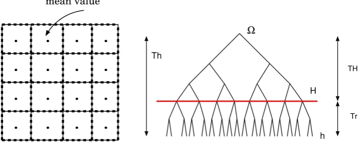
Example 5.2 Let us assume that Ω is decomposed into p = 16 subdomains Ω = Sp i=1Ωi. Sometimes these sub-domains Ωi are called cells. The set of nodal points on the interface is denoted by IΣ. HDD can compute the solution on the interface IΣ and the mean value

over each Ωi, i= 1, ..., p, (see Fig. 5.1).

.

.

.

.

.

.

.

.

.

.

.

.

.

.

.

.

mean value

Ω

h H

TH

Th

Tr

Figure 5.1: (left) HDD computes the solution on a coarse mesh (or the interface I(Σ)) and the mean value inside of each cell. (right) Algorithm “Leaves to Root” goes through the whole tree, but “Root to leaves” starts in the root, goes through a subtreeTTH and terminates

on a coarse level with the mesh sizeH (marked with the red horizontal line). After that the mean value inside of each coarse cell (of size H×H) is computed.

Example 5.3 To compute the FE solution uh(xi) in a fixed nodal point xi ∈ Ω, i.e., to define how the solution uh(xi) depends on the given FE Dirichlet data gh ∈ RI(∂Ω) and the FE right-hand side fh ∈RI(Ω).

5.1

Computing the mean value in all subdomains

ω

∈

T

Letωbe the father node,ω1the left son, andω2the right son. Thenω=ω1∪ω2,ω1∩ω2 6=∅,

with ω, ω1,ω2 ∈TTh. To simplify the notation, we will writedi :=dωi and (fi, gi) instead of

(fωi, gωi),i= 1,2 (see also Fig. 2.3). Recall the following notation (see (Eq. 3.16), (Eq. 3.17)):

d1 = (f1, g1) = (f1, g1,Γ, g1,γ), d2 = (f2, g2) = (f2, g2,Γ, g2,γ), where (5.2)

g1,Γ := (g1)|Γω,1, g1,γ := (g1)|γ, g2,Γ := (g2)|Γω,2, g2,γ := (g2)|γ.

(5.3)

We consider a linear functionalλω with the following properties:

λω(dω) = (λgω, gω) + (λfω, fω), (5.4)

λω(dω) = c1λω1(dω1) +c2λω2(dω2), (5.5)

where λg_ω :_RI(∂ω) →_R, λf_ω :_RI(ω) →_R, c1, c2 two constants, and (·,·) the scalar product of

two vectors.

Definition 5.1 Let ω1 ⊂ω, λfω1 :R

I(ω1)_→

R. a) We define the following extension of λfω1

(λf_ω1|ω₎ i :=

(λf_ω1)i for i∈I(ω1),

0 for i∈I(ω\ω1),

where (λf ω1|

ω_{) :}

RI(ω) → R. b) The extension of the functional λg1,Γ :RI(Γω,1) →R is defined

as

(λg_1,Γ|Γ)i :=

(λg_1,Γ)i for i∈I(Γω,1),

0 for i∈I(Γ\Γω,1),

where (λg_1,Γ|Γ_{) :}

RI(Γ)→R.

Definition 5.2 Using (Eq. 5.3), we obtain the following decompositions

λg_ω1 = (λg_1,Γ, λg_1,γ) and λg_ω2 = (λg_2,Γ, λg_2,γ), where λ₁g_,Γ :_RI(Γω,1)→

R, λg1,γ :RI(γ) →R,

λg_2,Γ :_RI(Γω,2) _→

R, λg2,γ :RI(γ)→R.

Lemma 5.4 Let λω(dω) satisfy (Eq. 5.4) and (Eq. 5.5) with ω=ω1∪ω2. Let λgω1, λ

g ω2, λ

f ω1

and λf

ω2 be the vectors for the representation of the functionals λω1(dω1) and λω2(dω2). Then

the vectors λf

ω, λgω for the representation

λω(dω) = (λfω, fω) + (λgω, gω), where fω ∈RI(ω), gω ∈RI(∂ω), (5.6)

are given by

λf_ω = ˜λf_ω+ (Φf_ω)Tλg_γ, λg_ω = ˜λg_ω+ (Φg_ω)Tλg_γ,

˜

λf_ω :=c1λfω1|

ω_+c

2λfω2|

ω_{, (5.7)}

˜

λg_Γ :=c1λg1,Γ|

Γ_+c

2λg2,Γ|

Γ_{, (5.8)}

Proof: Let dω1, dω2 be the given data and λω1 and λω2 be the given functionals. Then the

functionalλω satisfies

λω(dω)

(Eq.5.5)

= c1λω1(dω1) +c2λω2(dω2)

(Eq.5.4)

= c1((λfω1, f1) + (λ

g

ω1, g1)) +c2((λ

f

ω2, f2) + (λ

g

ω2, g2)).

Using the decomposition (Eq. 5.2), we obtain

λω(dω) = c1(λfω1, f1) +c2(λ

f

ω2, f2) +c1((λ

g

1,Γ, g1,Γ) + (λg1,γ, g1,γ)) (5.10) +c2((λg_2,Γ, g2,Γ) + (λg2,γ, g2,γ)). (5.11)

The consistency of the solution implies g1,γ =g2,γ =:gγ. From the Definition 5.1 follows

(λf_ω1, f1) = (λfω1|

ω

, fω), (λfω2, f2) = (λ

f ω2|

ω

, fω),

(λg_1,Γ, g1,Γ) = (λ

g

1,Γ|

Γ_{, g}

ω), (λ g

2,Γ, g2,Γ) = (λ

g

2,Γ|

Γ_{, g}

ω). Then, we substitute the last expressions in (Eq. 5.10) to obtain

λω(dω) = (c1λfω1|

ω

+c2λfω2|

ω

, fω) + (c1λ

g

1,Γ| Γ

+c2λ

g

2,Γ| Γ

, gω) (5.12)

+(c1λ

g

1,γ+c2λ

g

2,γ, gγ). Set ˜λf_ω :=c1λfω1|

ω_+c

2λfω2|

ω_{, ˜λ}g

Γ :=c1λ

g

1,Γ|

Γ_+c

2λ

g

2,Γ|

Γ_{and λ}g

γ :=c1λ

g

1,γ +c2λ

g

2,γ. From the algorithm “Root to Leaves” we know that

gγ = Φω(dω) = Φgω·gω+ Φfω·fω. (5.13) Substituting gγ from (Eq. 5.13) in (Eq. 5.12), we obtain

λω(dω) = (˜λfω, fω) + (˜λgω, gω) + (λgγ,Φ g

ωgω+ Φfωfω) = (˜λf_ω+ (Φf_ω)Tλg_γ, fω) + (˜λgω+ (Φ

g ω)

T_λg γ, gω). We define λf

ω := ˜λfω+ (Φfω)Tλgγ and λgω := ˜λgω+ (Φgω)Tλgγ and obtain

λω(dω) = (λfω, fω) + (λgω, gω). (5.14)

Example 5.5 Lemma 5.4 with c1 =

|ω1|

|ω|, c2 =

|ω2|

|ω| can be used to compute the mean values in all subdomains ω ∈TTh.

5.2

Algorithms for computing the mean values

Below we describe two algorithms which are required for computing the mean value in all subdomains ω ∈TTh. These algorithms compute vectors λ

g

ω and λfω respectively.

The initialisation is λg ω := ( 1 3, 1 3, 1

3), λ

f

ω := (0,0,0) for all leaves of TTh. Let us denote

λg₁ := λg_ω1, λg₂ := λg_ω2. The algorithms for building λg_ω and λf_ω for all ω ∈ TTh, which have

Algorithm 5.1 (Building of λg ω)

build functional g(λg₁, λg₂, Φg_ω,...)

begin

allocate memory for λg

ω;

for all i∈I(Γω,1) do

λg

ω[i]+ =c1λg1[i];

for all i∈I(Γω,2) do

λg_ω[i]+ =c2λ

g

2[i];

for all i∈I(γ) do

z[i] =c1λg1[i] +c2λg2[i];

v := (Φg_ω)T ·z;

for all i∈I(∂ω) do

λg

ω[i] := λgω[i] +v[i];

return λg_ω;

end;

Letλf₁ :=λf ω1, λ

f

2 :=λfω2.

Algorithm 5.2 (Building of λf_ω)

build functional f(λf₁, λf₂, Φf

ω,...) begin

for all i∈I(ω1\γ) do

λf

ω[i]+ =c1λf1[i];

for all i∈I(ω2\γ) do

λf_ω[i]+ =c2λf2[i];

for all i∈I(γ) do

z[i] =c1λf1[i] +c2λf2[i];

v := (Φf_ω)T ·z;

for all i∈I(ω) do

λf

ω[i] := λfω[i] +v[i];

return λf_ω;

end;

Remark 5.1 a) If only the functionals λω, ω ∈ TTh, are of interest, the maps Φω do not

need to be stored.

b) For functionals with local support in some ω0 ∈ TTh, it suffices that Φω is given for all

ω ∈ TTh with ω ⊃ ω0, while λω0(dω0) is associated with ω0 ∈ TTh. The computation of

Λ(uh) = λ(d) starts with the recursive evaluation of Φω for all ω ⊃ ω0. Then the data dω0

are available and λω0 can be applied.

5.3

Solution in a subdomain

Suppose that the solution is only required in a small subdomain ω ∈ TTh (Fig. 5.2, left).

computing the solution in ω. The storage requirements are also significantly reduced. We only store the mappings Φf_ω and Φg_ω for all ω ∈ TTh that belong to the path from the root

of TTh to ω. The storage requirement is O(nhlognh), where nh is the number of degrees

of freedom in Ω. The computational cost of the “Root to Leaves” is O(nhlog2nh). If the right-hand side is smooth, it can be discretized (defined) only on a coarse mesh TH (see Fig. 5.2, right). About the interpolation and restriction operators read in [31, 22, 7, 21].

ω

H h

Figure 5.2: (left) The solution in a subdomain ω ∈ TTh is required. HDD computes

subse-quently the solution only on the dotted lines and then only in ω; (right) The coarse H and the fineh scales.

6

Numerics

In [31, 7, 22], the HDD method was compared with the preconditioned conjugate gradient (PCG) method, with the hierarchical (H)- Cholesky method and the direct full H-matrix inverse. A cheap H-matrix approximation of the inverse, computed from the H-Cholesky factors, was used as a preconditioner.

Some experiments were performed with two meshes - a coarse for the right-hand side and a fine for the diffusion coefficient. Technical details and implementation of the HDD method can be found in [32, 7, 31]. The data misfit and the likelihood function in the Bayesian-like approach were computed in [58, 56, 45, 46, 53, 57]. In the following numerical experiments we compare the computational time and memory requirement of HDD with the times and memory requirements of the H-matrix inverse and theH-Cholesky factorisation.

We consider the problem as in Eq. 1.1 with fixed Z. The computational domain is a unit square Ω = [0,1]2_{, the diffusion coefficient isκ(x, y) = 1 + 0.5·sin(50x) sin(50y). Note,}

that HDD does not require an axes parallel triangulation. All numerical experiments were performed on a usual notebook. Figure 6.1 demonstrates the dependence of computing times (left) and memory requirements (right) on the H-matrix accuracy (see the adaptive rank arithmetic in [21]). One can see that the computational time and storage requirement of theH-Cholesky factorisation are the best. The HDD method shows a slightly larger time and storage than the H-Cholesky factorisation (due to some overhead) and is better than the directH-matrix inverse. Note that HDD computes more details about the operator and the solution than the H-Cholesky factorisation.

10-6 10-5 10-4 10-3

H-matix accuracy

0 20 40 60 80 100

time, sec.

H-Cholesky HDD H-inverse

10-6 10-5 10-4 10-3

H-matix accuracy

0 10 20 30 40 50

memory size, MB

H-Cholesky HDD H-inverse

Figure 6.1: Comparison of the HDD,H-Cholesky factorisation, and H-matrix inverse. (left) Dependence of the computing time (in sec.) and (right) memory requirements (in MB) on the H-matrix accuracy, n= 1292 _dofs.

In the next example we consider again the problem as in Eq. 1.1. The parameter Z is fixed and κ is a jumping coefficient as in Fig. 6.2 with α= 10−5 _{and β = 1. Such problems}

appear in the material sciences and in medicine (the, so-called, skin problem).

0 _{0.25 0.75} 1

0.5 1

4h

Figure 6.2: Model domain Ω = [0,1]2. The diffusion coefficient is very small (α = 10−5) inside the grey areas and large in white subdomains (β = 1).

Figure 6.3 compares the computational times of HDD and PCG methods. The PCG time includes the time needed for: (a) computing the stiffness matrix A in the H-matrix format; (b) computing the H-Cholesky decomposition of A (used as a preconditioner); (c) PCG iterations.

For example, for n = 66049, the PCG time is 53 = 38.2 + 11.4 + 3.4 (sec.). Note that for

n≈263000 dofs there is not enough memory to compute the stiffness matrixA and perform itsH-Cholesky factorization. The advantage of the HDD method is that it does not require an agglomeration of the whole stiffness matrix. The memory is dynamically allocated and deallocated.

In the next example we take a coarse mesh for the right-hand side with the grid step size

103 104 105 106 #ndofs

100 102

time, sec.

HDD PCG

Figure 6.3: HDD and PCG computing times vs. n. The accuracy in eachH-matrix subblock is 10−8_{, the PCG stopping criteria ε}

cg = 10−8, H_h = 2 as in Sec. 3.5.

Fig. 6.4(right). The accuracy inside of each H-matrix subblock is 10−5_{. Note, that PCG}

requires too much memory for n = 5132 _{dofs and we were not able to compute ˜u}

cg.

103 104 105

#ndofs

10-8 10-6 10-4 10-2

error

inf. norm Frob. norm

103 104 105 106

#ndofs 100

102

time, sec.

PCG HDD

Figure 6.4: Dependence of the absolute errors on the number of dofs, f = 1, α(x, y) = 1/(1.0001 + sin(500x) sin(500y)). H-matrix accuracy ε = 10−5_, H

h = 2. (left) errors (left) dependence of the errors ku˜cg−u˜k2 and ku˜cg−u˜k∞ on n; (right) computing times PCG and HDD vs. n.

Figure 6.5 shows the total storage requirement for all matrices Φg_ω and Φf_ω, ω∈TTh. We

see an almost linear dependence on n.

7

Conclusion and discussion

0 2 4 6 8

#dofs ₁₀4

0 2 4 6 8

memory size, MB

104

g

f

Figure 6.5: Dependence of the total memory requirement for all Φg

ωand Φfωonn, the maximal H-matrix rank is k = 7.

Bayesian approach. HDD can also be used when the simulated data and measurement data are compared (e.g., in regression, parameter inference, data assimilation, Kalman filter, and Bayesian update problems). HDD uses the fact that often only a functional of the solution or a small part of it is observed or measured. Therefore, HDD computes only a part of the inverse operator and only a part of the solution. Optimally, HDD computes only what is needed, i.e., what is measured.

As such the computational accuracy is as usual (for instance, as in the standard FEM method), but the computational recourses (FLOPS and storage) are smaller. The HDD method is based on the hierarchical (recursive) domain decomposition, FEM, and the Schur complement methods. If the forward operator and the right-hand side can be discretized on different meshes, which is often the case in multiscale problems, the HDD method can get significant advantages. The computational resources will be reduced even more.

Additionally, to speed up the Schur complement computations, we approximate all inter-mediate and auxiliary matrices in theH-matrix format. We then achieve the computational costO(nlog3n) and the storageO(nlog2n). There is some overhead due to the construction of the hierarchical decomposition tree TTh and permutation of indices.

To apply the HDD method, the user should have a possibility to 1) modify the assembling procedure of the stiffness matrix; 2) build the hierarchical domain decomposition tree.

We note that the interface size in a d-dimensional problem is O(nd−1_{). So in a 2D case,}

the interface is O(n), whereas, in 3D problems, the interface is O(n2). This fact results in increasing matrix sizes. The structure and the cost of the H-matrix arithmetics become more expensive too.

The HDD method can be coupled with more uncertainty quantification and parameter inference techniques. Potentially interesting could be the coupling with the Multi-Level Monte Carlo method.

Acknowledgments

References

[1] Tracy Babb, Adrianna Gillman, Sijia Hao, and Per-Gunnar Martinsson. An accelerated poisson solver based on multidomain spectral discretization. BIT Numerical Mathemat-ics, 58(4):851–879, 2018.

[2] I. Babuka, R. Tempone, and G.E. Zouraris. Galerkin finite element approximations of stochastic elliptic partial differential equations. SIAM Journal on Numerical Analysis, 42(2):800–825, 2004.

[3] R.D. Berry, H. N. Najm, B.J. Debusschere, H. Adalsteinsson, and Y.M. Marzouk. Data-free inference of the joint distribution of uncertain model parameters. Journal of Com-putational Physics, 231:2180–2198, 2012.

[4] H.-J. Bungartz and M. Griebel. Sparse grids. Acta Numer., 13:147–269, 2004.

[5] S. Dolgov, B. N. Khoromskij, A. Litvinenko, and H. G. Matthies. Computation of the response surface in the tensor train data format. arXiv preprint arXiv:1406.2816, 2014.

[6] S. Dolgov, B. N. Khoromskij, A. Litvinenko, and H. G. Matthies. Polynomial chaos ex-pansion of random coefficients and the solution of stochastic partial differential equations in the tensor train format. IAM/ASA J. Uncertainty Quantification, 3(1):1109–1135, 2015.

[7] F. Drechsler. Uber die L¨¨ osung von elliptischen Randwertproblemen mittels Gebietszer-legungstechniken, Hierarchischer Matrizen und der Methode der finiten Elemente. PhD thesis, PhD thesis, Universitaet Leipzig, Germany, 2016.

[8] T. A. El Moselhy and Y. Marzouk. Bayesian inference with optimal maps. Journal of Computational Physics, 231(23):7815–7850, 2012.

[9] M. Espig, W. Hackbusch, A. Litvinenko, H. G. Matthies, and Ph. W¨ahnert. Efficient low-rank approximation of the stochastic galerkin matrix in tensor formats. Computers and Mathematics with Applications, 67(4):818–829, 2014.

[10] M. Espig, W. Hackbusch, A. Litvinenko, H. G. Matthies, and E. Zander. Efficient analysis of high dimensional data in tensor formats. In Sparse Grids and Applications, pages 31–56. Springer, 2013.

[11] J. Galvis and M. Sarkis. Approximating infinity-dimensional stochastic darcy’s equa-tions without uniform ellipticity. SIAM Journal on Numerical Analysis, 47(5):3624– 3651, 2009.

[12] A. George. Nested dissection of a regular finite element mesh. SIAM J. Numer. Anal., 10:345–363, 1973. Collection of articles dedicated to the memory of George E. Forsythe.

[14] M. Goldstein and D. Wooff. Bayes Linear Statistics, volume 160 of Wiley Series in Probability and Statistics. Wiley, Chichester, UK, 2007.

[15] I. G. Graham, F. Y. Kuo, D. Nuyens, R. Scheichl, and I.H. Sloan. Quasi-Monte Carlo methods for elliptic PDEs with random coefficients and applications. J. Comput. Phys., 230(10):3668–3694, 2011.

[16] L. Grasedyck. Theorie und anwendungen hierarchischer matrizen. Ph.D. Thesis, Uni-versity of Kiel, Germany, 2001.

[17] L. Grasedyck and W. Hackbusch. Construction and arithmetics of H-matrices. Com-puting, 70(4):295–334, 2003.

[18] M. Griebel. Sparse grids and related approximation schemes for higher dimensional problems. In Foundations of computational mathematics, Santander 2005, volume 331 of London Math. Soc. Lecture Note Ser., pages 106–161. Cambridge Univ. Press, Cam-bridge, 2006.

[19] W. Hackbusch. Elliptic differential equations, volume 18 of Springer Series in Compu-tational Mathematics. Springer-Verlag, Berlin, 1992. Theory and numerical treatment, Translated from the author’s revision of the 1986 German original by Regine Fadiman and Patrick D. F. Ion.

[20] W. Hackbusch. A sparse matrix arithmetic based on H-matrices. I. Introduction to H-matrices. Computing, 62(2):89–108, 1999.

[21] W. Hackbusch. Hierarchical Matrices: Algorithms and Analysis. Springer Series in Computational Mathematics, Volume 49. Springer, 2015.

[22] W. Hackbusch and F. Drechsler. Partial evaluation of the discrete solution of elliptic boundary value problems. Computing and Visualization in Science, 15(5):227–245, Oct 2012.

[23] W. Hackbusch and B. N. Khoromskij. A sparse H-matrix arithmetic. II. Application to multi-dimensional problems. Computing, 64(1):21–47, 2000.

[24] W. Hackbusch, B. N. Khoromskij, and R. Kriemann. Hierarchical matrices based on a weak admissibility criterion. Computing, 73(3):207–243, 2004.

[25] B. N. Khoromskij and A. Litvinenko. Data sparse computation of the Karhunen-Lo`eve expansion. In AIP Conference Proceedings, volume 1048(1), pages 311–314. AIP, 2008.

[26] B. N. Khoromskij and Ch. Schwab. Tensor-structured Galerkin approximation of para-metric and stochastic elliptic PDEs. SIAM J. of Sci. Comp., 33(1):1–25, 2011.

[27] D. Kressner and Ch. Tobler. Low-rank tensor Krylov subspace methods for parametrized linear systems. SIAM J. Matrix Anal. Appl., 32(4):1288–1316, 2011.

[29] F. Y. Kuo, Ch. Schwab, and I. H. Sloan. Multi-level quasi-Monte Carlo finite element methods for a class of elliptic pdes with random coefficients. Foundations of Computa-tional Mathematics, pages 1–39, 2015.

[30] S. Le Borne, L. Grasedyck, and R. Kriemann. Parallel black box domain decomposi-tion based H −lupreconditioning. Max-Planck-Institut MIS, Leipzig, www.mis.mpg.de, Preprint 115:(electronic), 2005.

[31] A. Litvinenko. Application of hierarchical matrices for solving multiscale prob-lems. PhD Dissertation, Leipzig University, Germany, https://publications.rwth-aachen.de/record/754296, 2006.

[32] A. Litvinenko. Documentation for the HDD method. Technical report in Max-Planck-Institut MIS, Leipzig, Germany, www.mis.mpg.de/preprints/tr/index.html, 5, 2006.

[33] A. Litvinenko, R. Kriemann, M. G. Genton, Y. Sun, and D. E. Keyes. Hlibcov: Parallel hierarchical matrix approximation of large covariance matrices and likelihoods with applications in parameter identification. MethodsX, 7:100600, 2020.

[34] A. Litvinenko and H. G. Matthies. Inverse problems and uncertainty quantification. arXiv preprint arXiv:1312.5048, 2013.

[35] A. Litvinenko and H. G. Matthies. Numerical methods for uncertainty quantification and bayesian update in aerodynamics. InManagement and Minimisation of Uncertain-ties and Errors in Numerical Aerodynamics, pages 265–282. Springer Berlin Heidelberg, 2013.

[36] A. Litvinenko and H. G. Matthies. Uncertainty quantification and non-linear bayesian update of pce coefficients. PAMM, 13(1):379–380, 2013.

[37] A. Litvinenko, H.G. Matthies, and T. A. El-Moselhy. Sampling and low-rank tensor approximation of the response surface. In Josef Dick, Frances Y. Kuo, Gareth W. Peters, and Ian H. Sloan, editors, Monte Carlo and Quasi-Monte Carlo Methods 2012, volume 65 ofSpringer Proceedings in Mathematics &Statistics, pages 535–551. Springer Berlin Heidelberg, 2013.

[38] A. Litvinenko, Y. Sun, M. G. Genton, and D. E. Keyes. Likelihood approximation with hierarchical matrices for large spatial datasets. Computational Statistics & Data Analysis, 137:115 – 132, 2019.

[39] P.-G. Martinsson. The hierarchical poincar´e-steklov (hps) solver for elliptic pdes: A tutorial. arXiv preprint arXiv:1506.01308, 2015.

[40] Y. Marzouk, H. Najm, and L. Rahn. Stochastic spectral methods for efficient Bayesian solution of inverse problems. Journal of Computational Physics, 224(2):560–586, June 2007.

[42] Y. M. Marzouk and H. N. Najm. Dimensionality reduction and polynomial chaos ac-celeration of Bayesian inference in inverse problems. Journal of Computational Physics, 228(6):1862–1902, 2009.

[43] H. G. Matthies and A. Keese. Galerkin methods for linear and nonlinear elliptic stochas-tic partial differential equations. Computer Methods in Applied Mechanics and Engi-neering, 194(12-16):1295–1331, 2005.

[44] H. G. Matthies and E. Zander. Solving stochastic systems with low-rank tensor com-pression. Linear Algebra and its Applications, 436(10):3819–3838, 2012.

[45] H. G. Matthies, E. Zander, O. Pajonk, B. V. Rosi´c, and A. Litvinenko. Inverse problems in a Bayesian setting. InComputational Methods for Solids and Fluids Multiscale Anal-ysis, Probability Aspects and Model Reduction Editors: Ibrahimbegovic, Adnan (Ed.), ISSN: 1871-3033, pages 245–286. Springer, 2016.

[46] H. G. Matthies, E. Zander, B. V. Rosi´c, and A. Litvinenko. Parameter estimation via conditional expectation: a Bayesian inversion. Advanced Modeling and Simulation in Engineering Sciences, 3(1):24, 2016.

[47] H.G. Matthies, A. Litvinenko, O. Pajonk, B. V. Rosi´c, and E. Zander. Parametric and uncertainty computations with tensor product representations. In Andrew M. Dienstfrey and Ronald F. Boisvert, editors, Uncertainty Quantification in Scientific Computing, volume 377 of IFIP Advances in Information and Communication Technology, pages 139–150. Springer Berlin Heidelberg, 2012.

[48] A. Mugler and H.-J. Starkloff. On elliptic partial differential equations with random coefficients. Stud. Univ. Babes-Bolyai Math, 56(2):473–487, 2011.

[49] H. N. Najm, B.J. Debusschere, Y.M. Marzouk, S. Widmer, and O. P. Le Maˆıtre. Un-certainty Quantification in Chemical Systems. Int. J. Num. Meth. Eng., 80:789–814, 2009.

[50] F. Nobile, R. Tempone, and C. G. Webster. A sparse grid stochastic collocation method for partial differential equations with random input data. SIAM Journal on Numerical Analysis, 46(5):2309–2345, 2008.

[51] A. Nouy. A generalized spectral decomposition technique to solve a class of linear stochastic partial differential equations. Comput. Methods Appl. Mech. Engrg., 196(45-48):4521–4537, 2007.

[52] A. Nouy. Proper generalized decompositions and separated representations for the numerical solution of high dimensional stochastic problems. Archives of Computational Methods in Engineering, 17(4):403–434, 2010.

[54] M. Parno, T. Moselhy, and