Adaptive Resource Provisioning based on Application State

Adaptive Resource Provisioning based on

Application State

Constantine Ayimba

, Paolo Casari

, Vincenzo Mancuso

†_{IMDEA Networks Institute, Madrid, Spain,}∗_{University Carlos III of Madrid, Spain}

E-mail:†{name.surname}@imdea.org

Abstract—Infrastructure providers employing Virtual Network Functions (VNFs) in a cloud computing context need to find a balance between optimal resource utilization and adherence to agreed Service Level Agreements (SLAs). Tenants should be allocated as much computing, storage and network capacity as they need in order not to violate SLAs, but not more so that the infrastructure provider can accommodate more tenants to increase revenue. This paper presents an optimizer VNF that ensures that a given virtual machine (VM) is sufficiently utilized before directing traffic to another VM, and an orchestrator VNF that scales the number of VMs up or down as needed when workloads change, thereby limiting the number of active VMs to a minimum that can deliver the service. We setup a testbed to transcode and stream Video on Demand (VoD) as a service. We present experimental results which show that when the optimizer and orchestrator are used together they outperform static provisioning in terms of both resource utilization and service response times.

Index Terms—NFV, Provisioning, SLA, QoS, MANO

I. INTRODUCTION

Infrastructure providers often need to optimize their cloud computing resources to reduce costs while maintaining the Quality of Service (QoS) they provide to their customers [1]. This process typically involves assigning an optimal amount of resources to each tenant, so that spare capacity can remain available for other tenants. In this way, the provider can obtain more profit with modest resources. However this process is not trivial, given that the adherence to Service Level Agree-ment (SLA) constraints and the provisioning of a just sufficient amount of resources are often contending targets.

It is common practice in cloud networks to make use of more than one server to provide a given service to end users in order to guarantee better availability according to a given SLA [2]. This however means that the network owner incurs extra expenses without guarantees that the extra resources will actually be necessary. With Network Function Virtualization (NFV) such resources can be dynamically scaled up as needed to accommodate high demand, or scaled down when demand decreases.

This paper presents a dynamic scaling system that can be used by Management and Orchestration (MANO) [3] utilities to provision resources dynamically based on traffic demands. Concretely our main contributions are:

1) A load optimization network function that channels re-quests to alternative nodes only when the set of resources currently allocated is sufficiently highly utilized;

2) An orchestrator that scales Virtual Machine (VM) nodes up or down by predicting the system state through ap-proximations of near-term statistical state distributions. To illustrate the operation of the proposed provisioning scheme, we use transcoding as a case study of a cloud service. Transcoding is a resource-demanding process and is therefore a suitable application to be run as a service in the cloud. This is particularly important when the device on which the media is consumed has limited computational resources and power, as would be the case for a mobile phone.

The rest of this paper is organized as follows. In Section II, we briefly discuss previous work related to dynamic provision-ing. In Section III, we present key definitions and subsequently provide a detailed description of our system. In Section IV, we describe the experiments to test the proposed provisioning scheme, analyze the results and discuss their implications. Finally in Section V we conclude the paper and propose possible future areas of research.

II. RELATEDWORK

Several schemes have been proposed to tackle the chal-lenges posed by dynamic scaling. Iqbal et al. [4] propose a reactive model based on heuristics obtained from logs of HTTP servers to scale up resources and a polynomial regression model (trained on the logs) to predict when resources should be scaled down. Islam et al. [5] employ a neural network trained using data from the TPC-W [6] benchmarking tool and a sliding window to predict CPU utilization in a virtual machine in order to decide when scaling is required.

The authors of [7] propose admission control with schedul-ing that combines heterogeneous workloads (with high and low resource demands) to better utilize spare capacity that may otherwise remain unused when serving homogeneous work-loads. In [8], the authors propose a proportional thresholding policy that adapts to workloads so that a tenant can carry out horizontal scaling (increase the capacity of a service by adding resources). This scheme relies on monitoring tools that infrastructure providers offer to their tenants.

machines. They highlight the instability issues caused by the setting of improper thresholds, as well as by a too strict or too weak control.

Most of the approaches cited bear a huge overhead in training an intelligent agent with known workloads. Some of the proposals, as those in [7] and [9], are also fairly complex as they require fine-grained knowledge of cloud service delivery metrics. In contrast, our proposed system does not require prior knowledge of an application’s traffic demand as it adapts to changing workloads. In the design of our adaptation mechanism, we take into account the recommendations given in [10] such as the need to monitor the system prior to and after scaling in order to prevent oscillations in the VM instantiation process.

III. SYSTEMDESCRIPTION

A. Definitions

Adaptive provisioning can be considered a special case of sequential decision making [11]. An agent monitors the environment in order to obtain its state. It then decides on an action to take. Feedback from the environment, in the form of an immediate positive or negative reward signal or an eventual outcome, indicates how good or bad the action or a sequence of actions was. Such an action or sequence of actions results in a transition of the environment from one state to another.

If we let T be the set of decision epochs, S be the set of states the system can be in, As be the set of actions that the agent can take when the system is in state s,pt(·|s, a)be the distribution of system state changes given the state and action at the current decision epoch, following [12], we can formalize the sequential decision process as

{T, S, As, pt(·|s, a)}. (1)

B. System Functions

Our system uses discrete time epochs to make scaling decisions based on the current state of the system. A state refers to the number of requests being served concurrently by a VM node and will be used interchangeably throughout this paper. The actions to be taken are predefined based on an average system-wide value obtained by monitoring the set of active VM nodes for a finite time and counting the number of times each was servicing a specified number of requests.

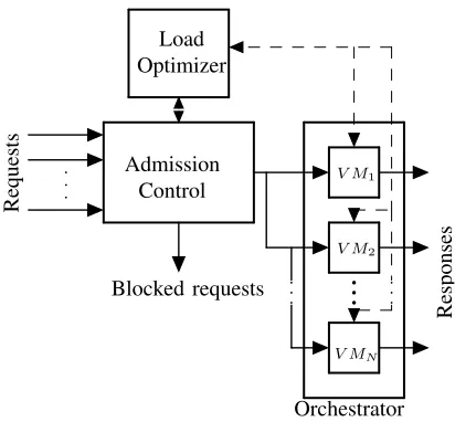
A block diagram of the transcoding Service Function Chain (SFC) is shown in Fig. 1. The admission control function carries out the instantaneous monitoring of individual nodes: it has the effect of converting each VM node into a finite-state machine, given that it conditionally admits requests based on the current state of the node, thereby limiting the number of possible states. An admitted request increases the state value of a VM node while a request that is fully served decreases the state value. Each of these events occurs with a probability that depends on the workload and computing power of the VM node respectively. These managed transitions can be modelled via a discrete-time Markov chain (DTMC). Systemic environment monitoring is carried out by the Orchestrator function.

V MN

Admission Control

Requests

Orchestrator

Responses

Blocked requests Load Optimizer

V M2 V M1

Fig. 1. Block diagram of transcoding service chain

1) Orchestrator: The orchestrator takes action in response to perceived system state as gleaned from polling the set of active VM Nodes. The actions that can be taken are:

• Scale up: Increase the number of active VM nodes to handle increased demand.

• Scale down: Reduce the number of active VM nodes when demand is low.

• No action: If the current number of active nodes can handle the traffic satisfactorily.

Scaling Up: The orchestrator employs a provisioning algo-rithm that calculates the average number of concurrent requests being served by the entire set of active VM nodes using reports they send. These are obtained over a time window that is at least an order of magnitude longer than the service time of a single request, and are sent at intervals slightly shorter than the observation window. This setting preserves the memory of traffic events in previous epochs, and reduces the possibility of premature system scaling, which may result in oscillations (scaling down shortly after scaling up, or vice-versa) [10].

The average number of concurrent requests being served, Kσ can be calculated as

Kσ = k X

i=0



i N(t)

X

j=1

wj(t)pij(t) 

, (2)

wherekis the size of the state space, N(t)is the number of active VM nodes in observation windowt,wj(t)is the fraction of counts in nodejw.r.t. the total counts from all active nodes taken over observation windowtandpij(t)is the probability a given VM node j is running i concurrent transcoding jobs over observation windowt.

cal-0 1 2 3 4 0

20 40 60 80 100

Concurrent transcoding requests

%

CPU

utilization

Median value Regression fit

Fig. 2. Relationship between CPU Utilization and concurrent transcoding processes in a VM. CPU usage is monitored by querying the number of ongoing transcoding requests.

culated experimentally when the system is close to saturation. Specifically, the orchestrator checks if

Kσ ≥K∆ , K∆=

Pk i=0iπi

γ , (3)

whereK∆is the upper bound metric,γis a tunable parameter,

and πi is the long-term probability of being in state i (the long-term probabilities,π, are derived from the state transition matrix of a VM node operating under saturation conditions). If the condition in (3) is verified, a new VM node is added to the set of VM nodes.

The tradeoff between the blocking probability and resource utilization is not trivial. The choice of γ should be such that the orchestrator only adds to the set of VM nodes when the joint utilization of the current set is high enough. Similarly, γ should be chosen such that the orchestrator is responsive to perceptible changes in demand that may lead to reduced service availability, owing to an increase in the likelihood that a new request finds all active VM nodes too busy to admit it (blocking probability). In a scenario with known rates of arrival and departures the blocking probability can be computed using a queue model for instance, however we use observations to make the system more robust to dynamic demands.

Scaling Down: A lower bound metric, K∇ of system utilization also needs to be established, which specifies the lowest average number of concurrent processes that can justify the use of extra resources. It is fittingly chosen in relation to K∆ as

K∇=ηK∆ , 0< η <1 , (4)

whereη is a tuning parameter specifying the tolerance of the system.

Should Kσ become lower than K∇, we determine which node should be shut down by computing the average number of concurrent processes,K(n), for each node:

K(n) = min

1≤n≤N k X

i=0

ipin , (5)

Load Balancer Requests

Load Optimizer and Orchestrator Physical Servers

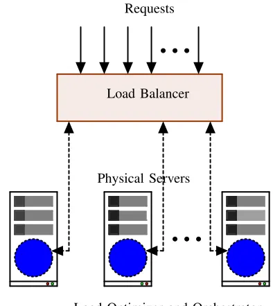
Fig. 3. Schematic of large scale deployment.

wherepin is the probability of being in statei for VM node n, N is the total number of active VM nodes and k is the size of the state space. The VM nodeˆn= arg min_nK(n)is scheduled for shutdown.

No Action: If the state of the system is such that: K∇ < Kσ < K∆, no scaling action is undertaken.

2) Load Optimizer and Admission Control: Our system includes a load-optimizer network function which informs the decision of the admission controller to admit or drop a request. Given the strong correlation depicted in Fig. 2, the optimizer obtains the utilization level of each of the active VM nodes in turn by querying the number of concurrent requests in service. If the utilization of a VM node is such that a new request will not cause it to saturate, the optimizer directs the admission controller to admit the new request to the given VM node. If all the active VM nodes are saturated, the optimizer instructs the admission controller to drop the new request. Therefore, unlike a fair load balancer which channels traffic uniformly among nodes, the load optimizer only redirects requests to an alternative node when the ones under consideration are saturated or near saturation.

C. Large Scale Deployments

Though the experiments outlined in this paper were carried out on a single server, large scale deployments can be handled in a modular fashion as shown in Fig 3. Here, a set of VNFs is employed in each physical server, and a standard load balancer mediates the channeling of the traffic to each server.

IV. EXPERIMENTALRESULTS

A. Testbed Setup

Fig. 4. Testbed setup. (1) Host PC (2) Client PCs (3) Gigabit per second (Gbps) capable switch.

Each of the client PCs has at least 2 hyperthreaded cores (4 logical CPUs) and 8 GB RAM. The host uses KVM [13] as the hypervisor and libvirt [14] to manage the deployment of the VM nodes. Each VM Node is configured with 4vCPUs and 2GB of RAM.

The host launches VM nodes running G-Streamer [15] as the transcoder. It also runs ancillary Python and Shell scripts which handle the signalling and control aspects ensuring that each response is correctly mapped to the requesting process running on the client PCs. The Admission Control, Load Optimizer and the Orchestrator Network Functions are located in the host. All physical and virtual machines run on Ubuntu Linux 16.04 LTS.

We obtained the source video files from the official “Big Buck Bunny” repository [16] in 3 formats/resolutions: avi (720p), h264 (1080p), h264 (2160p). These formats rep-resent mature standards widely adopted by content providers for video encoding [17]. We subsequently carried out scene selection and length splitting to create short video segments of 5 seconds for each file, using FFMPEG [18], without changing the source formats or other properties. This is common prac-tice in adaptive bit rate streaming, whereby the same video content is encoded in different resolutions and file formats that support fragmentation. Each short fragment can be streamed interchangeably with others (bearing the same content but of a different format/resolution) depending on available network bandwidth [19].

Each request specifies the source file to transcode from the three formats/resolutions. The format of the output stream is selected randomly by the control script as VP8 with either 320x180 or 640x360 resolution. The audio stream is transcoded from 448 kbps AC-3 format with 6 channels (5.1 surround) to 128 kbps mp3 audio with 2 channels (stereo). These formats were chosen for their popularity in video streaming [20]. For each request, the time taken to complete the simultaneous transcoding and streaming operation (as reported by G-Streamer) is logged with a timestamp indicating when it was received.

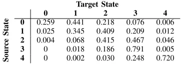
TABLE I

TRANSITION PROBABILITIES OF A BUSYVM NODE

Target State

0 1 2 3 4

Sour

ce

State

0 0.259 0.441 0.218 0.076 0.006

1 0.025 0.345 0.409 0.209 0.012

2 0.004 0.068 0.415 0.467 0.046

3 0 0.018 0.186 0.791 0.005

4 0 0.002 0.030 0.248 0.720

B. System calibration

In order to establish the upper-bound metric,K∆, the SFC

was constrained to use only one VM node. This threshold was obtained by running transcoding requests at random intervals between 0 and 5 seconds of each other for a sustained period of 16 hours. This rate ensured that the VM node was operating close to saturation for the entire duration. The admission control was set to only admit new requests if CPU utilization was below saturation.

A monitoring script, running at 1 second intervals, keeps track of the process IDs of ongoing transcoding streams, in order to obtain the probabilities of transitioning from one state to another. The script checks the process IDs of running transcoder threads and compares the set of current IDs with the previous set. The intersection of the two sets indicates the number of transcoding processes that were ongoing in the system, the number of IDs present in the current set but absent in the previous set indicates the new requests. The number of IDs absent in the new but present in the previous set indicates completed streams. The total number of parallel transcodings in progress define the state.

Table I shows the transition probabilities obtained with our testbed. Using (3) and the stationary distribution derived from Table I, we computed K∆ = 2.709_γ . State occupancy

reports were obtained over a duration of 5 minutes and sent to the orchestrator every 3 minutes to provide some filtering to spurious traffic events which may result in premature scaling [10].

The blocking probability is calculated as the proportion of requests that are not admitted over the 3 minute epoch to the total number of requests received in that epoch.

C. Results and Discussion

In the referenced figures, “LO” refers to the case where only the Optimizer (with all three nodes active) is used and not the Orchestrator whilst “LB” refers to the case where Load Balancing (round robin) is applied with all three VM nodes active.

0 20 40 60 80 100 120 0

0.2 0.4 0.6

Reference Time (min)

Blocking

Probability

γ= 1.0 γ= 1.2 γ= 1.4

γ= 1.8 LO LB

Fig. 5. Blocking probabilities under different values ofγ. Between minute 10 and 20 the average traffic is 23 requests/min. Between minute 70 and 90 the average traffic is 20 requests/min. The rest of the time the average traffic is 8 requests/minute.η= 0.8.

0 20 40 60 80 100 120

0 1 2 3 4

Reference Time(min)

Number

of

VM

Nodes

γ= 1.0 γ= 1.2 γ= 1.4 γ= 1.8

Fig. 6. Scaling actions by orchestrator. Given that only 3 VM nodes were available, scaling to a 4thVM node is included to show that if the capacity of the host had not been exceeded then there would have been another VM node added to the active set.η= 0.8.

0 20 40 60 80 100 120

0 20 40 60 80 100

Reference Time (min)

%CPU

utilisation

γ= 1.0 γ= 1.2 γ= 1.4 γ= 1.8 LO,VM1 LO,VM2

LO,VM3 LB

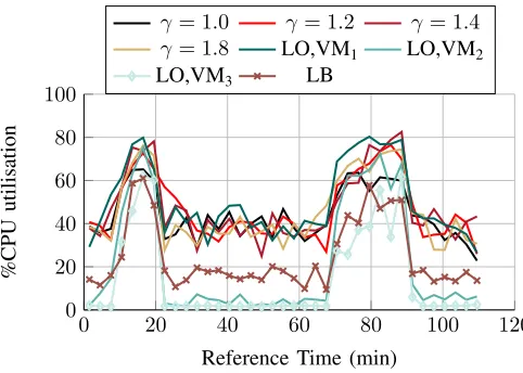
Fig. 7. CPU utilization. Between minute 10 and 20 the average traffic is 23 requests/min. Between minute 70 and 90 the average traffic is 20 requests/min. The rest of the time the average traffic is 8 requests/minute. Except for the “LB“ and “LO“ case VM2 and VM3 are shut down at certain periods, see

Fig. 6.η= 0.8.

Fig. 6 shows the number of VM nodes dynamically pro-visioned by the orchestrator. A higher setting of γ increases the sensitivity of the orchestrator resulting in more scaling actions as the SFC adjusts to subtler changes in demand. When γ = 1.0, the orchestrator exhibits the smallest sensitivity and no scaling action is made leaving only the primary VM node to handle all the traffic.

Fig. 7 shows the average CPU utilization of the primary node (VM1) for different values ofγ, and that of all VMs for

the two cases in which the orchestrator is not used. At low demand, when only the Load Optimizer (LO) is used, VM1

experiences most of the traffic while VM2and VM3are mostly

idle. In the case where the orchestrator is used together with the optimizer, it shuts down the least busy VM nodes thereby eliminating superfluous resources. When Load Balancing (LB) is used, the levels of CPU utilization at low demand are about

15 20 25 30 35 40 45 50

0 0.2 0.4 0.6 0.8 1

Transcoding time (s)

CDF

γ= 1.0 γ= 1.2 γ= 1.4 γ= 1.8 LO LB

Fig. 8. Distribution of Service times for transcoding h264(1080p) to VP8(640x360). The other input and output formats mentioned in Section IV show similar results.

50% less than those experienced when the load optimization is used together with the orchestrator.

Fig. 8 shows the distribution of the service times of transcoding requests. The greater the number of active nodes, the worse the service time, given that more context switch-ing [21] has to be performed (whereby the hypervisor has to stop, save state, handle interrupts and resume processing on a VM Node), which results in less CPU time for performing the transcoding. Context switching compounds when the hypervi-sor manages multiple VM nodes. The orchestrator ameliorates this effect by shutting down idle VM nodes resulting in improved performance.

The median transcoding time with γ = 1.8 (which pro-vides a good compromise between service times and service availability) is about 1.3 s shorter than when round-robin load balancing (LB) is used. When extra VM nodes are not added, as is the case withγ= 1.0, the best response is observed.

with reference to SLA terms agreed with tenants.

V. CONCLUSIONS

In this paper, we presented a load optimizing and an orches-trator network function. When used together in a SFC, they improve the utility of VM nodes involved in servicing requests and limit the use of resources to those strictly necessary to meet SLAs.

We demonstrated that by learning the response of virtual machines handling a cloud service, decision bounds can be obtained for scaling up or down. We also showed that shutting down under-utilized nodes improves service times by reducing hypervisor overheads involved in managing multiple virtual machines.

As future extensions to this work, we plan to use online machine learning to appropriately adjustγandη. This should reduce the blocking probability by making scaling more agile and able to face rapidly-varying network traffic.

ACKNOWLEDGMENTS

This work has received funding from the European Union’s Horizon 2020 research and innovation programme under GA No. 732667 (RECAP), and from the Spanish Ministry of Sci-ence, Innovation and Universities grant DisCoEdge (TIN2017-88749-R). The work of V. Mancuso was supported by a Ramon y Cajal grant (RYC-2014-16285) from the Spanish Ministry of Economy and Competitiveness.

REFERENCES

[1] Y. Xia, M. Zhou, X. Luo, Q. Zhu, J. Li, and Y. Huang, “Stochastic modeling and quality evaluation of infrastructure-as-a-service clouds,”

IEEE TASE, vol. 12, no. 1, Jan 2015.

[2] E. J. Ghomi, A. M. Rahman, and N. N. Qader, “Load-balancing algorithms in cloud computing: A survey,”Elsevier JNCA, vol. 88, no. 1, June 2017.

[3] R. Mijumbi, J. Serrat, J. l. Gorricho, S. Latre, M. Charalambides, and D. Lopez, “Management and orchestration challenges in network functions virtualization,” IEEE Communications Magazine, vol. 54, no. 1, Jan 2016.

[4] W. Iqbal, M. N. Dailey, D. Carrera, and P. Janecek, “Adaptive resource provisioning for read intensive multi-tier applications in the cloud,”

Elsevier FGCS, vol. 27, no. 6, June 2011.

[5] S. Islam, J. Keung, K. Lee, and A. Liu, “Empirical prediction models for adaptive resource provisioning in the cloud,”Elsevier FGCS, vol. 28, no. 1, Jan 2012.

[6] D. A. Menasce, “TPC-W: a benchmark for e-commerce,”IEEE Internet Computing, vol. 6, no. 3, May 2002.

[7] S. K. Garg, A. N. Toosi, S. K. Gopalaiyengar, and R. Buyya, “SLA-based Virtual Machine Management for Heterogeneous Workloads in a Cloud Datacenter,”Elsevier JNCA, vol. 45, Oct 2014.

[8] H. C. Lim, S. Babu, J. S. Chase, and S. S. Parekh, “Automated Control in Cloud Computing: Challenges and Opportunities,” inProc. ACM ACDC, Barcelona, Spain, June 2009.

[9] J. Bi, H. Yuan, W. Tan, M. Zhou, Y. Fan, J. Zhang, and J. Li, “Application-aware dynamic fine-grained resource provisioning in a virtualized cloud data center,”IEEE TASE, vol. 14, no. 2, April 2017. [10] X. Dutreilh, A. Moreau, J. Malenfant, N. Rivierre, and I. Truck, “From

data center resource allocation to control theory and back,” in Proc. IEEE ICCC, Miami, FL, July 2010.

[11] M. L. Littman, “Algorithms for sequential decision making,” Ph.D. dissertation, Brown University, Providence, RI, Mar 1996.

[12] L. P. Kaelbling, M. L. Littman, and A. R. Cassandra, “Planning and acting in partially observable stochastic domains,”Elsevier ARTIFICIAL INTELLIGENCE, vol. 101, 1998.

[13] A. Kivity, Y. Kamay, D. Laor, U. Lublin, and A. Liguori, “KVM: the Linux Virtual Machine Monitor,” inProc. OLS, Ottawa, Canada, July 2007.

[14] M. Bolte, M. Sievers, G. Birkenheuer, O. Nieh¨orster, and A. Brinkmann, “Non-intrusive Virtualization Management Using Libvirt,” in Proc. DATE, Leuven, Belgium, Mar 2010.

[15] “Gstreamer open source multimedia framework,” https://gstreamer.freedesktop.org, accessed: 2018-07-11.

[16] “Big Buck Bunny,” http://bbb3d.renderfarming.net/download.html, ac-cessed: 2018-07-11.

[17] N.-M. Nguyen, D.-H. Bui, N.-K. Dang, E. Beigne, S. Lesecq, P. Vivet, and X.-T. Tran, “An Overview of H.264 Hardware Encoder Architec-tures Including Low-Power FeaArchitec-tures,”JEC, vol. 4, June 2014. [18] “FFmpeg,” https://www.ffmpeg.org, accessed: 2018-07-11.

[19] D. K. Krishnappa, M. Zink, and R. K. Sitaraman, “Optimizing the video transcoding workflow in content delivery networks,” inProc. ACM MMSys, Portland, Oregon, Mar 2015.

[20] Y. O. Sharrab and N. J. Sarhan, “Detailed comparative analysis of vp8 and h.264,” inProc. 2012 IEEE ISM, Irvine, CA, Dec 2012.