Multi-Physics Modeling of Light-Limited
Microalgae Growth in Raceway Ponds
Andreas Nikolaou∗,∗∗ Peter Booth∗ Fraser Gordon∗ Junfeng Yang∗ Omar Matar∗ Benoˆıt Chachuat∗,∗∗ ∗Department of Chemical Engineering, Imperial College London,
South Kensington Campus,London SW7 2AZ, UK.
∗∗Centre for Process Systems Engineering, Imperial College London,
South Kensington Campus,London SW7 2AZ, UK.
Abstract: This paper presents a multi-physics modeling methodology for the quantitative prediction of microalgae productivity in raceway ponds by combining a semi-mechanistic model of microalgae growth describing photoregulation, photoinhibition and photoacclimation, with models of imperfect mixing based on Lagrangian particle tracking and heterogeneous light distribution. The photosynthetic processes of photoproduction, photoregulation and photoinhibition are represented by a model of chlorophyll fluorescence developed by Nikolaou et al. (2015), which is extended to encompass photoacclimation. The flow is simulated with the commercial CFD package ANSYS, whereas light attenuation is described by the Beer-Lambert law as a first approximation. Full-scale simulation results are presented on extended time horizons. Comparisons are made in terms of areal productivities under both imperfect and idealized (CSTR) mixing conditions, and for various extraction rates and water depths.
Keywords:microalgae; raceway pond; photoinhibition; photoacclimation; CFD; imperfect mixing; light attenuation
1. INTRODUCTION
Phototrophic microorganisms—both microalgae and cyanobacteria—show a great potential for industrial applications, including food, pharmaceuticals and cosmetics, chemicals, and even biofuels. In comparison to conventional oil crops, they are independent from arable land and fresh water and can accumulate an array of useful by-products (Milledge, 2011). Moreover, lab- and pilot-scale experiments have shown that many microalgae species can achieve primary productivities orders of magnitude larger than terrestrial oil crops. The main commercial applications of microalgae so far have been concerned with high-value products, including carotenoids and omega-3 and omega-6 polyunsaturated fatty acids (Leu and Boussiba, 2014). In contrast, the commercial viability of microalgae as biofuel feedstock is still uncertain and calls for the development of large-scale outdoor raceway ponds to reduce production costs (Wijffels and Barbosa, 2010). Estimating the productivity of such systems based on a crude extrapolation from lab-scale experiments may be misleading due to drastically different conditions regarding access to light and nutrient, alongside imperfect mixing and temperature variations. In this context, mathematical modeling is a great help to understand, and in turn remedy, the gap between lab-scale observations and the industrial-scale reality (B´echet et al., 2013; Bernard et al., 2016). Not only are these models useful for analyzing and optimizing actual production systems, but they could also drive the choice ⋆ This work was financial supported by Marie Curie Career
Integra-tion Grant PCIG09-GA-2011-293953 (DOP-ECOS).
of a particular microalgae species that is best suited to the local environment or even to a particular season.
The modeling of high-density microalgae culture systems proves more challenging than that of bacterial or yeast culture systems. Part of this added complexity stems from the wide range of mechanisms that microalgae use to respond and adapt to light and other local environment factors, including photoregulation and photoacclimation whose dynamics range from seconds to days. Another challenge is tied to the fact that access to light inside the culture medium is highly heterogeneous due to light absorption, scattering and shadowing effects. Depending upon the mixing conditions, microalgae cells may be exposed to a range of different light irradiance levels over time scales of seconds or minutes—in addition to the diurnal light cycle.
Light Attenuation
Biological Model
0 100 200 300 400 500 600 700
0 200 400 600 800 1000 1200
Irradiance
Time
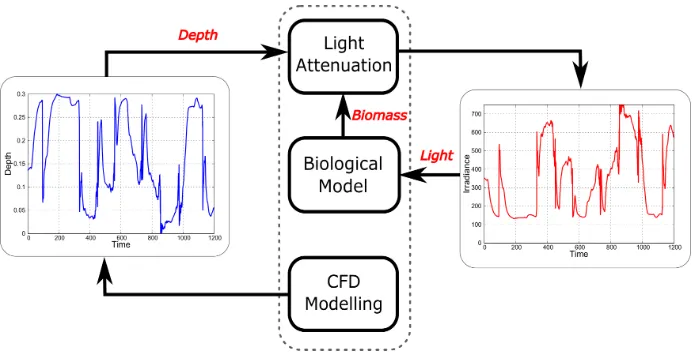
Fig. 1. Coupling methodology of photosynthesis kinetics, hydrodynamics and light attenuation in the raceway pond.
This paper proposes an improved multi-physics model of microalgae raceway ponds by combining a semi-mechanistic model of microalgae growth describing pho-toregulation, photoinhibition and photoacclimation, with models of imperfect mixing based on Lagrangian particle tracking and heterogeneous light distribution. This model and the coupling methodology are presented in Sect. 2. The algal growth kinetics are based on the chlorophyll fluorescence model by Nikolaou et al. (2015) and fea-ture a novel extension to account for photoacclimation. Moreover, the flow is simulated with the commercial CFD package ANSYS, whereas light attenuation is described by the Beer-Lambert law as a first approximation. The numerical implementation is discussed in Sect. 3, before presenting full-scale simulation results on extended time horizons. Comparisons are made in terms of areal pro-ductivities under both imperfect and idealized (CSTR) mixing conditions, and for various extraction rates and water depths. Finally, Sect. 4 concludes the paper.
2. MULTI-PHYSICS MODELING METHODOLOGY
The overall modeling methodology is depicted in Fig. 1. A commercial CFD package (ANSYS) is used to simulate the velocity field inside the raceway pond, and subse-quently obtain a large number of particle trajectories for which light histories are generated via the light attenua-tion model. These light histories are then passed to the biological model in order to predict primary production along the individual trajectories. The overall productivity of the raceway pond is obtained by averaging over all the trajectories. The following two simplifications are adopted in order to make the coupling sequential and tractable: (i) the velocity field is unaffected by the microalgae cells in suspension; and (ii) the concentration and composition of microalgae cells inside the pond is uniform in terms of their light attenuation effect. Moreover, we consider nutrient-replete conditions and assume no limitation by CO2 or temperature for the scope of this paper.
2.1 Microalgae Growth Kinetics
The model by Nikolaou et al. (2015) predicts fluorescence fluxes by taking into account the state of the photosystem II (RCII) and the activity of photoregulation (NPQ).
These fluxes can then be related to the growth rate as (Bernardi et al., 2015, 2016)
µ=
Iσν AηP
1 +ηD+ηqEα+AηP+CηI − R
θ (1)
˙
A= −I σPS2A+ B
τ (2)
˙
B=I σPS2A−B
τ +krC−kdσPS2I B (3) ˙
C= −krC+kdσPS2I B (4)
ΦA
f =
1
1 +ηP+ηD+ηqEα
(5)
ΦB
f =
1
1 +ηD+ηqEα (6)
ΦCf =
1
1 +ηI+ηD+ηqEα (7)
˙
α=ξ α− I
n
In
qE+In
!
(8)
σPS2=
σηP
N(1 +ηD+ηqEα+ηP)
(9)
The growth rate µ [s−1] in Eq. (1) is proportional to the chlorohpyll-to-carbon quota, θ [gchlgC−1]. It is also a function of the incoming light intensity,I [µE m−2s−1], the total cross-section,σ[m2gchl] and the respiration rate parameter,R[gCgchl−1s−1], where asν is a stoichiomet-ric coefficient between electron flow and carbon fixation. Following the model by Han (2002), Eqs. (2)-(4) describe transitions of the reaction centers of photosystem II (RCII) between active,A[−], occupied,B[−] and damaged,C[−] states, as a function ofI. Photoproduction is described by the transitionA ⇀↽ B, which depends on the effective cross section,σPS2[m2µE−1] and turnover time, τ [s] of RCII. Photoinhibition is described by the transition B ⇀↽ C, which depends on damage, kd [−] and repair, kr [s−1]
constants. The fluorescence quantum yields for each RCII state, ΦA
f [−], ΦBf [−] and ΦCf [−] given by Eqs. (5)-(7), depend on the dimensionless parameters ηP, ηD, ηI and ηqE. The NPQ activity,α[−] in Eq. (8) tracks a sigmoidal set-point function ofI, with parametersIqE [µE m−2s−1] and n[−]. Finally, Eq. (9) relates σPS2 with the number of RCII,N [µE g−1
Table 1. Estimated acclimation and respiration parameter values.
Parameter Calibrated value Units
δ 1.38×10⁻¹ −
θ0 3.60×100 gchlg−1
C
κ −1.89×10⁻¹ −
N0 1.71×100 µE g−1
chl
λ 1.22×10⁻¹ −
IqE,0 8.13×10² µE m−2s−1
ǫ 4.48×10⁻¹ −
R 1.78×10⁻⁵ gCg−1
chls−
1
Bernard (2011) argues that photoacclimation dynamics can be described in terms of variations of the so-called acclimation irradiance,Ig [µE m−2s−1] as
˙
Ig=δ(I−Ig)µ , (10)
where δ [–] is a constant proportionality coefficient rep-resenting the rate of photoacclimation. The link between Eq. (10) and the kinetic model (1)-(9) is established through empirical acclimation rules that relate the vari-ablesθ,N andIqE to the acclimation state,Ig:
• The variation in the pigment content of the cells due to photoacclimation is described by power laws relating the chlorophyll-to-carbon quota, θ and the number of RCII, N to the acclimation state, Ig as (Fisher et al., 1996; MacIntyre et al., 2002; Nikolaou et al., 2016)
θ=θ0(Ig)κ, (11)
N=N0(Ig)λ, (12)
with acclimation parametersθ0,N0, κandλ. • The variation in the carotenoid-to-chlorophyll ratio
of the cells due to photoacclimation impacts the dissipation of excess energy via NPQ regulation and is captured by a simple linear law relatingIqEwithIg as (Simionato et al., 2011)
IqE=IqE,0+ǫIg, (13) with corresponding acclimation parametersI0 andǫ.
The rationale behind the choice of the acclimation rules (11)–(13) is that they provide a minimal model complexity for accurate prediction of a set of experimental data for the microalga Nannochloropsis gaditana, while still providing statistically confident estimates.
The overall growth model (1)-(13) accounts for photopro-duction, photoregulation, photoinhibition and photoaccli-mation all together, and its dynamics span many time-scales ranging from milliseconds to days. Due to space restriction we only report the estimated values of the extra acclimation and respiration parameter in Table 1 and refer the reader to Nikoalou (2015) for further details; the remaining parametersηD, ηP, ηI, ηqE, τ, kd, kr, ξ, n, σare set to the values given in Nikolaou et al. (2015).
2.2 Hydrodynamics
Modeling of the flow conditions inside the raceway pond is carried out in the commercial package ANSYS 15 (http:
//www.ansys.com/), based on an existing raceway pond at
INRA Narbonne, France (Hreiz et al., 2014). This raceway is equipped with a paddlewheel (Fig. 2) and the water depth is set toH = 0.3 m (liquid volume of 15.8 m3) for the
Fig. 2. Geometrical characteristics of the raceway pond.
simulation. A tetrahedral structured mesh with 209,960 nodes and 183,615 elements is used for the 3-d simulation, which allows for a vertical discretization of the liquid phase into 20 layers. This mesh is further divided into two parts: (i) a finely discretized, sliding mesh of cylindrical shape surrounding the paddle-wheel and rotating around its axis at an angular velocity of 10 rpm; and (ii) a stationary mesh including the remaining computational domain. The code FLUENT is used to solve the Reynolds averaged Navier-Stokes equations in transient mode, with a time step of 0.01 s. The implicit compressive scheme of the volume of fluid (VOF) model is used to track the free surface of water and air, which has a surface tension coefficient of 71.99 mN m−1 at 25◦C. The realizableκ-ǫmodel with default parameter values is used to represent turbulence, the convective terms are discretized using the QUICK scheme, and the diffusion terms are central-differenced.
The simulation itself is divided into two parts.
(1) During the first 1,200 seconds of the simulation, the raceway pond is initialized from a resting state to a stabilized flow. The velocity field at 0.2 m above the raceway floor at the end of this period is illustrated in Fig. 3. The flow is turbulent near the paddlewheel and mostly laminar elsewhere. The inner bends of the pond are seen to cause a flow acceleration, whereas dead zones develop near the outer bends and at the inner side of the channel opposite the paddle-wheel.
Fig. 3. Mean velocity magnitude at 0.2 m above the raceway floor.
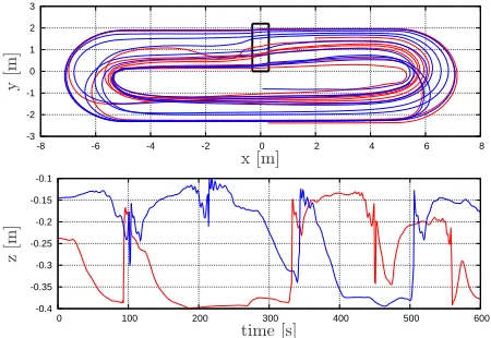
initialized with the velocity of the flow at their points of injection. Two selected trajectories are represented in Fig. 4 during 600 seconds, where the depth of the particles is seen to fluctuate considerably. The most important factor affecting the vertical position is the paddle-wheel rotation, which can push a particle up or down, depending on its position as it nears the paddles. The bends of the pond are also found to have an effect on the vertical position of the particles due to local velocity gradients.
-3 -2 -1 0 1 2 3
-8 -6 -4 -2 0 2 4 6 8
-0.4 -0.35 -0.3 -0.25 -0.2 -0.15 -0.1
0 100 200 300 400 500 600
x [m]
y
[m
]
z
[m
]
time [s]
Fig. 4. horizontal position (upper plot) and depth histories (lower plot) for two selected trajectories.
2.3 Light Attenuation
Since the commercial viability of microalgae production systems calls for denser cultures, accouting for light atten-uation is indeed paramount. As a first approximation, the light attenuation caused by both absorption by pigments and scattering by biomass particles may be predicted using Beer-Lambert’s law as (Bernard, 2011)
Iz=I0exp (−[Es(X+Xd) +EaXθ]z), (14) where I0 and Iz [µE m−2s−1] stand for the light
inten-sities at the surface and at a depth z [m] inside the culture, respectively. The light attenuation in Eq. (14) increases with the active and dead biomass concentra-tions, X and Xd [gCL−1], and with the chlorophyll con-centration, Xθ [gchlL−1]. The proportionality coefficient Ea [m2gchl−1] accounts for light absorption by pigment molecules, whereas Es [m2gC−1] accounts for light scat-tering by biomass particles. These coefficients are set to Ea = 0.20×10² m2gC−1 and Es= 0.10×10² m2gchl−1 thereafter, in agreement with the light attenuation ranges given by Sevilla and Grima (1997). Moreover, the incoming light intensity is set to follow a diurnal pattern given by the sinusoidal function
I0(t) =Imax
1−cos 864002πt
3
8 , (15)
with the mid-day irradiance Imax = 1200 µE m−2s−1 representative of Southern Europe during the summer.
2.4 Multi-Physics Coupling
Imperfect Mixing Case In order to simulate the raceway pond at scale, the idea is to integrate the microalgae growth model (1)-(13) through time along each Lagrangian
trajectory j = 1, . . . , Ntraj. Subsequently, the state vari-ables in the growth model are indexed withj in reference to the jth trajectory, such asµj(t), θj(t), Ig,j(t), and the
depth and local irradiance histories are denoted by zj(t)
andIj(t) likewise.
Following mass conservation principles, the local variations in active and dead biomass concentrations, Xj(t) and
Xd,j(t) are given by
˙
Xj(t) = (µj(t)−D)Xj(t), (16)
˙
Xd,j(t) =R Xj(t)−D Xd,j(t), (17)
whereD [s−1] is the dilution rate. Then, per the assump-tion that the concentraassump-tion and composiassump-tion of microalgae cells inside the pond are uniform in terms of their light at-tenuation effect, the coupling between the growth kinetics and the light attenuation along each trajectories follows from Eq. (14) in the form
Ij(t) =I0(t) exp −[Es(X(t) +Xd(t)) +EaX(t)θ(t)]zj(t)
, where the average active and dead biomass concentrations, X(t) andXd(t), and the average chlorophyll quota,θ, are calculated over all the Lagrangian trajectories as
X(t) = 1 Ntraj
Ntraj
X
j=1
Xj, Xd(t) =
1 Ntraj
Ntraj
X
j=1 Xd,j,
θ(t) = 1 Ntraj
Ntraj
X
j=1 θj(t).
The corresponding areal (net) primary productivity, P [gCL−1s−1] for the pond is given by
P(t) = 1 Ntraj
Ntraj
X
j=1
µj(t)Xj(t), (18)
and possibly averaged over a 24-hour period to obtain the daily-average (net) primary productivity.
Perfect Mixing (CSTR) Case In addition to the assump-tion of a uniform biomass concentraassump-tion and composiassump-tion with regards to light attenuation, this idealized case as-sumes that the microalgae cells are all identical in terms of their photosynthetic states. Unlike the imperfect mixing case above where the cells follow separate depth and light histories along the Lagrangian trajectories, perfect mixing considers for all the cells to have an equi-probable exposure to light across the water column.
The average photosynthetic state of the cells is described by integro-differential equations of the form
˙
Ig(t) = 1 H
Z H
0
δ[Iz(t)−Ig(t)]µ(t) dz ,
with Iz as given in Eq. (14), and the like for the other
averaged quantitiesµ, A, B, . . .in Eqs. (1)-(13). Then, the average active and dead biomass concentrations,X(t) and Xd(t) are obtained from
˙
X(t) = (µ(t)−D)X(t), ˙
Xd(t) =R X(t)−D Xd(t),
3. RESULTS AND DISCUSSIONS
The multi-physics model based on Lagrangian particle tracking and heterogeneous light distribution is comprised of a large set of differential equations, for which a merical solution can be obtained with state-of-the-art nu-merical integrators such as CVODE-SUNDIALS (https:
//computation.llnl.gov/casc/sundials/). In order to
run simulations on extended time horizons of several weeks, the Lagrangian trajectories computed with ANSYS (timespan of 1,200 seconds) are applied repeatedly based on a randomization over all the available trajectories at the paddle-wheel. Using a variable-order BDF method with a diagonal approximation of the Jacobian matrix and tight relative and absolute local error tolerances of, respectively, 10−7and 10−10, a one-day simulation of the raceway takes about 210 CPU-seconds with Ntraj = 200 Lagrangian trajectories and 570 CPU-seconds with Ntraj = 500 on a recent laptop computer.1 Moreover, no appreciable dif-ferences are observed for results computed with 200 tra-jectories or more.
The results of a full-scale dynamic simulation of the race-way pond are shown in Fig. 5 for a constant dilution rate of D= 0.25 day−1and water depth ofH = 0.30 m, and with an initial (active) biomass concentration of 100 mgCL−1. Both the active and dead biomass concentration profiles reach a cyclic steady-state regime—due to the diurnal light pattern imposed through Eq. (15)—within several weeks of simulated time; as light attenuation in the cul-ture increases with the concentrations of active and dead biomass, the rate of increase in active biomass during day-time progressively slows down until the point that it is balanced by the rate of respiration. Moreover, the daily variations in active biomass are expectedly larger than those in dead biomass, given that biomass decay occurs steadily during the day, unlike biomass growth.
0 0.5 1 1.5 2 2.5 3
0 0.1 0.2 0.3 0.4 0.5 0.6
0 5 10 15 20 25 30 35 40 45 50
t[day]
X
[gC
L
−
1]
Xd [gC
L
−
1]
Perfect mixing Imperfect mixing
Fig. 5. Evolution of the active (top plot) and dead (bottom plot) biomass over 50 days for the multi-physics model under either imperfect or perfect mixing.
Under imperfect mixing conditions, the daily average concentration of active and dead biomass reach ca. 1 Intel Core i7-3687U CPU @2.10GHz×4, running Ubuntu 14.04 LTS 64 bits and gcc version 4.8.4.
410 mgCL−1and 100 mgCL−1, respectively. These values are 6 to 7-fold lower than their counterparts in the ideal-ized case of perfect mixing, respectively, ca. 2630 mgCL−1 and 610 mgCL−1. These results thus provide a clear con-firmation that a large part of the loss in microalgae pro-ductivity that is observed in going from lab to industrial scale is attributable to imperfect mixing.
0 0.1 0.2 0.3 0.4 0.5 0.6 0.7 0.8 0.9 1
0.10 0.15 0.20 0.25 0.30 0.35
D[day−1]
X
[gC
L
−
1]
H= 0.2 m H= 0.3 m H= 0.4 m
Fig. 6. Active biomass concentrations at cyclic steady-state (24-hour average) for operations at various di-lution ratesD and water depths H.
A comparison of the realizable active biomass concentra-tions for various dilution rate values D in the range 0.1-0.4 day−1and water depthsH between 0.2-0.4 m is shown in Fig. 6. Note that different water depths are simulated here via direct scaling of the trajectory depth histories from the CFD base case ofH = 0.3 m, instead of recom-puting the Lagrangian trajectories anew for H = 0.2 m and 0.4 m. At a given dilution rate, the realizable biomass concentration decreases as the water depth increases due to the effect of light attenuation through the water col-umn. Overall, these projections show that cultures ofN. gaditana denser than 1 gCL−1 may hardly be grown in traditional raceways.
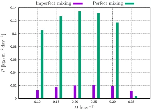
Quite remarkably, the realizable areal net productivities— computed from Eq. 18—turn out to be equal for all three water depths. These areal productivities are plot-ted in Fig. 7 for various dilution rates, under both im-perfect and im-perfect mixing conditions. In either cases, the areal productivity passes through a maximum for a dilution rate between 0.2-0.25 day−1. This maximum is ca. 20 gCm−2day−1 in the imperfect mixing case, which is again about 7-fold lower than the predicted value of 135 gCm−2day−1 under a perfect mixing scenario. As-suming (dry) biomass to have a carbon content of 50%, this gives an areal biomass productivity for the pond around 0.04 kg m−2day−1, which is close to the projected productivity of 0.035 kg m−2day−1 by Chisti (2007).
0 0.02 0.04 0.06 0.08 0.1 0.12 0.14
0.10 0.15 0.20 0.25 0.30 0.35
D[day−1]
P
[k
gC
m
−
2d
ay
−
1]
Perfect mixing Imperfect mixing
Fig. 7. Net primary production at cyclic steady-state (24-hour average) for the multi-physics model with imperfect mixing compared to the idealized perfect mixing case at various dilution ratesD.
a uniform biomass concentration in the raceway is sup-ported by experimental observations in Hreiz et al. (2014), although it may not hold for bigger raceways. Lastly, it is worth reemphasizing that the projected productivities are inherently optimistic as microalgae growth is both nutrient- and temperature-limited in practice.
4. CONCLUSIONS AND FUTURE DIRECTIONS
The proposed modeling framework is the first of its kind to couple a detailed algal growth kinetic model describing photoregulation, photoinhibition and photoacclimation all together, with a CFD model of imperfect mixing based on Lagrangian particle tracking and heterogeneous light distribution. This allows for realistic extrapolation of lab-scale measurements based on fluorometry and respirome-try to full-scale production in raceway ponds. Such extrap-olation capability may find applications for the screening of microalgae strains or even to guide the development of mutants for improved productivities in targeted geo-graphical regions. This generic simulation capability may also find applications in design and operations optimiza-tion of raceway ponds. As part of future work, it will be interesting to extend the present framework to encompass both nutrient- and temperature-limited growth for more realistic predictions.
REFERENCES
B´echet, Q., Shilton, A., and Guieysse, B. (2013). Modeling the effects of light and temperature on algae growth: State of the art and critical assessment for productivity prediction during outdoor cultivation. Biotechnol. Adv., 31(8), 1648–1663.
Bernard, O. (2011). Hurdles and challenges for modelling and control of microalgae for CO2 mitigation and biofuel production. J.
Process Control, 21(10), 1378–1389.
Bernard, O., Mairet, F., and Chachuat, B. (2016). Modelling of microalgae culture systems with applications to control and optimization. Adv. Biochem. Eng. Biotechnol., 153, 59–87. Bernardi, A., Nikolaou, A., Meneghesso, A., Morosinotto, T.,
Chachuat, B., and Bezzo, F. (2015). A framework for dynamic modeling of PI curves in microalgae.Comput. Aided Chem. Eng., 37, 2483–2488.
Bernardi, A., Nikolaou, A., Meneghesso, A., Morosinotto, T., Chachuat, B., and Bezzo, F. (2016). High-fidelity modelling methodology of light-limited photosynthetic production in mi-croalgae.PLoS ONE, in press.
Chisti, Y. (2007). Biodiesel from microalgae.Biotechnol. Adv., 25(3), 294–306.
Fisher, T., Minnaard, J., and Dubinsky, Z. (1996). Photoacclimation in the marine alga Nannochloropsis sp. (eustigmatophyte): A kinetic study. J. Plankton Res., 18(10), 1797–1818.
Han, B.P. (2002). A mechanistic model of algal photoinhibition induced by photodamage to photosystem-II. J. Theor. Biol., 214(4), 519–27.
Hartmann, P., Combe, C., Rabouille, S., Sciandra, A., and Bernard, O. (2014). Impact of hydrodynamics on single cell algal photosyn-thesis in raceways: characterization of the hydrodynamic system and light patterns. InProc. 19th IFAC World Congress. Hreiz, R., Sialve, B., Morchain, J., Escudi´e, R., Steyer, J.P., and
Guiraud, P. (2014). Experimental and numerical investigation of hydrodynamics in raceway reactors used for algaculture. Chem.
Eng. J., 250, 230–239.
Leu, S. and Boussiba, S. (2014). Advances in the production of high-value products by microalgae.Ind. Biotechnol., 10(3), 169–183. MacIntyre, H.L., Kana, T.M., Anning, T., and Geider, R.J. (2002).
Photoacclimation of photosynthesis irradiance response curves and photosynthetic pigments in microalgae and cyanobacteria.J.
Appl. Phycol., 38(1), 17–38.
Marshall, J.S. and Sala, K. (2011). A stochastic Lagrangian approach for simulating the effect of turbulent mixing on algae growth rate in a photobioreactor. Chem. Eng. Sci., 66(3), 384–392.
Milledge, J.J. (2011). Commercial application of microalgae other than as biofuels: a brief review. Rev. Environ. Sci. Biotechnol., 10(1), 31–41.
Nikoalou, A. (2015). Multi-scale Modeling of Light-limited Growth
in Microalgae Production Systems. Ph.D. thesis, Dpt. Chemical
Engineering, Imperial College London, UK.
Nikolaou, A., Bernardi, A., Meneghesso, A., Bezzo, F., Morosinotto, T., and Chachuat, B. (2015). A model of chlorophyll fluorescence in microalgae integrating photoproduction, photoinhibition and photoregulation.J. Biotechnol., 194, 91–99.
Nikolaou, A., Hartmann, P., Sciandra, A., Chachuat, B., and Bernard, O. (2016). Dynamic coupling of photoacclimation and photoinhibition in a model of microalgae growth.J. Theor. Biol., 390, 61–72.
Olivieri, G., Gargiulo, L., Lettieri, P., Mazzei, L., Salatino, P., and Marzocchella, A. (2015). Photobioreactors for microalgal cul-tures: A Lagrangian model coupling hydrodynamics and kinetics.
Biotechnol. Progr., 31(5), 1259–1272.
Pruvost, J., Cornet, J.F., and Legrand, J. (2008). Hydrodynamics influence on light conversion in photobioreactors: An energetically consistent analysis. Chem. Eng. Sci., 63(8), 1648–1663.
Sevilla, J. and Grima, E.M. (1997). A model for light distribution and average solar irradiance inside outdoor tubular photobioreactors for the microalgal mass culture. Biotechnol. Bioeng., 55(5), 701. Sheth, M., Ramkrishna, D., and Fredrickson, A.G. (1977). Stochastic
models of algal photosynthesis in turbulent channel flow.AIChE J., 23(6), 794–804.
Simionato, D., Sforza, E., Corteggiani Carpinelli, E., Bertucco, A., Giacometti, G.M., and Morosinotto, T. (2011). Acclimation
of Nannochloropsis gaditana to different illumination regimes:
Effects on lipids accumulation. Bioresour. Technol., 102(10), 6026–6032.
Sukenik, A., Levy, R.S., Levy, y., Falkowski, P.G., and Dubinsky, Z. (1991). Optimizing algal biomass production in an outdoor pond: a simulation model. J. Appl. Phycol., 3, 191–201.
Wijffels, R.H. and Barbosa, M.J. (2010). An outlook on microalgal biofuels.Science, 329(5993), 796–799.