Analyzing the Efficiency of Horizontal Photovoltaic Cells in Various Climate Regions

http://www.sciencepublishinggroup.com/j/jenr doi: 10.11648/j.jenr.20190802.15

ISSN: 2330-7366 (Print); ISSN: 2330-7404 (Online)

Analyzing the Efficiency of Horizontal Photovoltaic Cells in

Various Climate Regions

Parker Alan Hines, Torrey John Wagner

*

, Clay Michael Koschnick, Steven James Schuldt

Department of Systems Engineering & Management, Air Force Institute of Technology, Wright-Patterson Air Force Base, United States of America

Email address:

*

Corresponding author

To cite this article:

Parker Alan Hines, Torrey John Wagner, Clay Michael Koschnick, Steven James Schuldt. Analyzing the Efficiency of Horizontal Photovoltaic Cells in Various Climate Regions. Journal of Energy and Natural Resources. Vol. 8, No. 2, 2019, pp. 77-86. doi: 10.11648/j.jenr.20190802.15

Received: April 15, 2019; Accepted: May 23, 2019; Published: June 10, 2019

Abstract:

This research presents the development of linear regression models to predict horizontal photovoltaic power output. We collected a dataset from 14 global Department of Defense (DoD) installations over a timeframe of one year using an experimental apparatus, resulting in 24,179 usable data points. We developed a linear model to predict power output, which incorporated site-specific weather and geographical characteristics, along with Köppen-Geiger climate classifications in order to determine the effect of adding climate to the model. After performing a Wald test between the full model and a reduced model without Köppen-Geiger climate variables, it was determined that including Köppen-Geiger climate variables improved the model’s ability to account for horizontal photovoltaic power variation by 3%. Although adding Köppen-Geiger variables provided added value when modeling the training dataset, these variables were less effective in predicting the validation dataset. From the analysis, the ideal Köppen-Geiger region was determined to be a warm temperate main classification, a fully humid precipitation classification and a warm summer temperature classification. This region possessed a 30% greater average power production than the mean value of the base climate classification. We found that the cost-effectiveness of a photovoltaic array depends on Köppen-Geiger climate regions, in addition to weather characteristics and the orientation of the array.

Keywords:

Köppen-Geiger, Photovoltaic Cells, Linear Regression, Renewable Energy, Energy Resilience

1. Introduction

While weather variable effects on photovoltaic power production are discussed frequently in literature, there is limited information regarding the impact of the climate classification zone [1]. The few studies that have looked at climate’s effect on photovoltaic power production are based upon fixed-angle arrays instead of real-world data collected from horizontal systems [2]. With new technology being developed based on horizontal arrays, such as solar pavements, organizations with a global presence could benefit from an analysis showing the effect of climate region on the energy produced from horizontal PV panels.

Therefore, the purpose of this research effort was to determine the correlation between the power output of horizontal polycrystalline PV panels and the

Köppen-Geiger climate classification system. This involves analyzing data collected from test systems placed in various climate regions to determine the most beneficial areas for photovoltaic investment.

This study built upon prior research efforts that identified candidate test sites, completed the system design, assembled the experimental test equipment, and shipped the test equipment to 38 locations worldwide [3–5]. More information regarding these areas is provided in the remainder of this section.

1.1. Site Selection

however, the 2006 Kottek et al. version was used for this research because it had the highest number of climate regions [7]. The Köppen-Geiger system categorizes climate into five major climate zones: arid, warm temperate, snow, polar, and equatorial. Each zone has several types and subtypes based on precipitation and temperature. There are six precipitation classifications: desert, steppe, fully humid, summer dry,

winter dry, and monsoonal; and eight temperature

classifications: hot arid, cold arid, hot summer, warm summer, cool summer, extremely continental, polar frost, and polar tundra [6–10].

In designing this experiment, Nussbaum performed an analysis of variance (ANOVA) on the latitude and longitude of 1,763 DoD installations and found concentrations of installations in 25 distinct regions [3]. Then, a Pareto analysis was conducted to determine the climate regions that have the highest amount of installations. The Pareto analysis showed the DoD had installations in 14 of the 31 distinct Köppen-Geiger climate classifications. Test locations were selected based on these analyses, and then test systems were constructed and shipped to these locations. With spare parts, one additional test system was set up near Wright-Patterson Air Force Base, OH, USA to facilitate the diagnosis of system malfunctions. The final test location sites are shown as red dots on the map in Figure 1. Some of the locations in Figure 1 are close to one another, making it appear as one dot—e.g., the U.S. Air Force Academy and Peterson, AFB are both located near Colorado Springs, CO, USA.

Figure 1. Test site locations [5].

1.2. Test Equipment

Figure 2. Test system with monocrystalline PV panel (lower left),

polycrystalline panel (upper left), battery (black, lower right), weatherized case (yellow, lower right) and charging panel (upper right).

The main components of the system consisted of an

ALEKO 25 Watt, 12 Volt mono-crystalline solar panel, a Renogy 50 Watt, 12 Volt poly-crystalline solar panel, a Raspberry Pi 3, model B, version 1.2 computer inside a weatherized case, a weather probe, and an external power source, as shown in Figure 2. The system was also equipped with red, yellow, and green light emitting diodes (LED) to indicate an error had occurred within the system, the system was operational, and a reading was taking place, respectively. The external power source used to run the Raspberry Pi was provided by a 20-foot extension cord connected to an outdoor power source or by an additional PV panel and battery. The Raspberry Pi computer took measurements at 15-minute intervals [11-12]. These measurements included the current and voltage of the panels, ambient air temperature, and humidity of the site. The current was read using a noninvasive current Hall sensor [13]. Next, voltage was measured by the voltage drop across a known resistance. Finally, ambient air temperature and humidity were measured using a probe located on the outside of the weatherized case. Data collection was conducted using a micro secured digital (SD) card.

To ensure conformity and ease of system setup, each installer was instructed to place their systems in a flat orientation. This zero-degree tilt angle enables the data to be applied to potential solar pavement applications. To ensure that each panel received the maximum amount of sunlight per day, participants were instructed to place the systems so they would have a clear view toward the southern, eastern, and western horizons. Finally, participants were instructed to check system function once each day and to ensure the systems were clear of debris, snow or high amounts of dust.

2. Methodology

2.1. Data Collection and Configuration

Of the original 38 test sites, data was only received from 28 locations. After reception, the data had to be configured and compiled in order to provide a proper format for analysis. During each 15-minute interval, 64 readings for voltage and current were recorded for each panel, respectively. After multiplying these values together, the maximum power value was obtained for each interval. Next, the time for every location was adjusted from military or “Zulu” time to its respective time zone. Zulu time was the default time setting on each Raspberry Pi computer.

Upon completion of data compilation, other variables were incorporated with the dataset to support further analysis. Location-specific variables added to the dataset include latitude, altitude, Köppen-Geiger climate classification, and cloud ceiling obtained from the National Oceanic and Atmospheric Administration [14]. Each cloud ceiling measurement was matched to the closet 15-minute interval using RStudio statistical software.

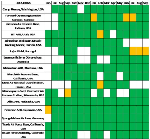
16-month collection period or because of errors in the date and time stamp of the recordings. The dates of the dataset ranged from June 2017 to September 2018, with 528,569 total data points. The data collected for each site can be seen in Figure 3.

Next the dataset was narrowed further to remove outliers and errors. The first discrepancy observed was the power output recorded for the mono-crystalline panel. The values ranged from 0 W to 500 W for a 25 W rated panel. Over 64,000 readings were higher than 50 W, and it is unlikely for the panel to consistently read at such a high output. As a result, this data was removed, and no further analysis was performed on the mono-crystalline panel. Next, Learmonth Solar Observatory in Northwestern Australia was removed because it was the only site in the southern hemisphere. Capturing differences between the hemispheres, such as the opposite seasons, could have complicated the model and risked having key variables excluded. After removal, the model’s final application and interpretation would be limited to the northern hemisphere.

Figure 3. Preliminary analysis site selection. A green filled box represents

one month of data, a yellow filled box represents approximately a half month of data, and an empty or white box represents three or less days of data or no data recorded at all.

Following the removal of Learmonth, a calibration break-in period for several locations was identified, and the discrepancies were removed. These periods were identified by comparing histograms of power, plotted against month and hour for every location. These histograms displayed high power recordings during night along with power recordings above the poly-crystalline panel’s rating of 50 W. However, these high recordings only occurred during the first several months of data collection, see Figure 4. Eventually, the power recordings behaved in a normal manner with readings of 1 W or less at night and no recordings above 40 W.

The last discrepancy identified if the data was associated with low temperature readings. The lowest temperature that

was recorded was -40°C. However, these readings appeared to be associated with an error because it was recorded at southern sites such as Jonathan Dickinson Missile Tracking Station in Florida. For this reason, data with temperature readings lower than -39.3°C were removed. Along with these low temperature readings, there were several high temperature and power readings that were removed due to these points being extreme outliers and were easily identified as errors.

Figure 4. Final analysis site selection. Locations’ discrepancies can be

identified with red, while blue represents reliable data and white represents three or less days of data or no data record at all.

2.2. Model Variables

After collecting and filtering the data, individual variables were considered to create a simplistic model that allowed for easy interpretation and could be applied to all sites. First, the final variables for the model were selected. These variables included poly-crystalline panel power output, test site latitude, Köppen-Geiger climate classification, altitude, month, hour, temperature, cloud ceiling, and humidity. Next the rational for the inclusion of each variable into the model will be discussed.

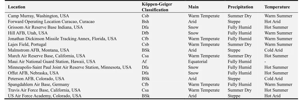
lower than 0.25 W were eliminated from the data readings. Latitude was the next variable incorporated into the model and was treated as a continuous variable measured in degrees. Latitude was selected to account for the angle of the sun’s irradiance. The ideal angle for the irradiance to strike the panel in order to maximize the area exposed is 90° [18]. This ideal angle is why many fixed solar panels are tilted at an angle equivalent to their latitude because irradiance strikes a horizontal panel directly at 90° at 0° latitude on the equator. Köppen-Geiger climate classifications were included in the model to identify how effective they predict solar panel power production. Climate classification can account for location-specific characteristics that may not be included in other variables, such as wind speed, precipitation, vegetation and geographical landmarks such as mountains. The Köppen-Geiger climate classification along with each sub classification for every site location is shown in Table 1. Other weather variables, such as temperature, cloud ceiling, and humidity, were added to the model due to their effect on solar power production. Temperature affects how efficient the panel is at generating power while cloud ceiling affects how

much irradiance the panel receives [14, 19–23]. Humidity affects both the efficiency of the panel and the amount of irradiance the panel receives. This is because the water vapor in the air affects the amount of diffuse irradiance that reaches the panel and humidity can also have a soiling effect on the panel if water vapor seeps into the glass casing [24–26]. The Köppen-Geiger climate classifications were treated as categorical variables while temperature, cloud ceiling, and humidity were treated as continuous variables. Temperature was measured in degrees, cloud ceiling in hundreds of feet, and humidity was expressed as a percentage.

Next, altitude was incorporated into the model to help account for the intensity of the irradiance on the panel. As irradiance travels to Earth, it can be deflected and diffused by water vapor and other particles in the air [26]. As altitude increases there is a lower chance for irradiance to be deflected and diffused resulting in a higher amount of direct irradiance hitting the solar panel compared to panels at lower altitudes. Altitude was measured in meters measured from sea level and treated as a continuous variable.

Table 1. Test site Köppen-Geiger climate classifications.

Location Köppen-Geiger

Classification Main Precipitation Temperature

Camp Murray, Washington, USA Csb Warm Temperate Summer Dry Warm Summer

Forward Operating Location Curacao, Curacao Bsh Arid Steppe Hot Arid

Grissom Air Reserve Base Indiana, USA Dfa Snow Fully Humid Hot Summer

Hill AFB, Utah, USA Dfb Snow Fully Humid Warm Summer

Jonathan Dickinson Missile Tracking Annex, Florida, USA Cfb Warm Temperate Fully Humid Warm Summer

Lajes Field, Portugal Csb Warm Temperate Summer Dry Warm Summer

Malmstrom AFB, Montana, USA BSk Arid Steppe Cold Arid

March Air Reserve Base, California, USA Csa Warm Temperate Summer Dry Hot Summer

Maui Air National Guard Station, Hawaii, USA Af Equatorial Fully Humid -

Minneapolis-Saint Paul Joint Air Reserve Station, Minnesota, USA Dfa Snow Fully Humid Hot Summer

Offut AFB, Nebraska, USA Dfa Snow Fully Humid Hot Summer

Peterson AFB, Colorado, USA BSk Arid Steppe Cold Arid

Spangdahlem Air Base, Germany Cfb Warm Temperate Fully Humid Warm Summer

Travis Air Force Base, California, USA Csa Warm Temperate Summer Dry Hot Summer

US Air Force Academy, Colorado, USA BSk Arid Steppe Hot Arid

Finally, time was incorporated into the model to account for the position of the sun throughout the day and its seasonal affects. Time was accounted for by using the variables hour and month. Hour accounted for the position of the sun as it traverses the sky from east to west across the panel. Minute was not included because the position of the sun does not change significantly between the 15-minute measurements compared to its position after 60 minutes. As a result, hour was treated as a categorical variable with values between 0-23. The time frame for this model was further limited between 10:00AM and 3:00PM or daylight hours. Creating a standard time frame helped eliminate bias in variable coefficients when the sun was not present due to northern locations having a shorter daylight period during the winter solstice [27]. Month helped account for seasonal changes throughout the year as well as the sun’s elevation in the sky with reference to the southern horizon. Month was also treated as a categorical variable with values between 1-12. After consolidating the data within the ranges of each

variable, the final dataset consisted of 24,179 data points and 14 test sites (Curacao did not have any cloud ceiling measurements). In conclusion, these variables aided in analyzing the effect of climate classification on horizontal solar panel power output while holding influential variables constant.

2.3. Analysis

The full and reduced models were compared using RStudio and conclusions were made on the effectiveness of the Köppen-Geiger climate classification system to predict photovoltaic power output compared to weather data.

The conceptual model can be seen in Equation 1--it identifies three specific factors that impact photovoltaic power production as expressed earlier in the paper. These factors can be broken into specific variables to better understand their influence on power, as shown in Equation 2. This equation contains 28 variables and associated

coefficients. The variables grouped together represent categorical variables that have multiple dummy variables. Dummy variables are equivalent to 0 or 1 in an equation such that one category is represented at a time. There is also one less dummy variable than there are categories for each group due to one variable being the baseline, which is taken into account by the intercept or β0. Finally, each numbered coefficient is defined in Table 2 below. Equation (1) is the conceptual photovoltaic power prediction model. Equation (2) is the statistical photovoltaic power prediction model.

power = f(sun angle, weather, climate) (1)

Y= β₀+β₁X₁+β₂X₂+β₃₋₁₃X₃₋₁₃+β₁₄₋₁₈X₁₄₋₁₈+β₁₉X₁₉+β₂₀X₂₀ +β₂₁X₂₁+ β₂₂₋₂₇X₂₂₋₂7 (2)

Table 2. Statistical Mode Coefficient Definitions.

Coefficient Variable Coefficient Variable

β₀ Intercept β₁₄ Hour 11 (11:00 AM)

β₁ Latitude β₁₅ Hour 12 (12:00 PM)

β₂ Altitude β₁₆ Hour 13 (1:00 PM)

β₃ Month: 2 (Feb) β₁₇ Hour 14 (2:00 PM)

β₄ Month: 3 (Mar) β₁₈ Hour 15 (3:00 PM)

β₅ Month: 4 (Apr) β₁₉ Temperature

β₆ Month: 5 (May) β₂₀ Humidity

β₇ Month: 6 (Jun) β₂₁ Cloud Ceiling

β₈ Month: 7 (Jul) β₂₂ Climate: Bsk

β₉ Month: 8 (Aug) β₂₃ Climate: Cfb

β₁₀ Month: 9 (Sep) β₂₄ Climate: Csa

β₁₁ Month: 10 (Oct) β₂₅ Climate: Csb

β₁₂ Month: 11 (Nov) β₂₆ Climate: Dfa

β₁₃ Month: 12 (Dec) β₂₇ Climate: Dfb

Next, assumptions were tested to determine if the proposed

model could be viable. Assumptions that were tested include multicollinearity, serial correlation, normality, homoscedasticity, and coefficient significance. These were all tested in RStudio to determine if further analysis could be carried out. If these assumptions were not met, appropriate measures needed to be taken to draw valid conclusions from the model.

After all assumptions were tested, a reduced model was created for both weather and climatic variables in order to conduct the Wald test. The Wald test compared these reduced models to the full model to determine if the variables provided any value in the prediction of power. The reduced models can be seen below in Equation 3 and 4.

Equation (3) is the reduced prediction model without Köppen-Geiger climate classifications.

Y= β₀ + β₁X₁ + β₂X₂ + β₃₋₁₃X₃₋₁₃ + β₁₄₋₁₈X₁₄₋₁₈ + β₁₉X₁₉ + β₂₀X₂₀ + β₂₁X₂₁ (3)

Equation (4) is the reduced prediction model without weather variables.

Y= β₀ + β₁X₁ + β₂X₂ + β₃₋₁₃X₃₋₁₃ + β₁₄₋₁₈X₁₄₋₁₈ + β₂₂₋₂₇X₂₂₋₂7 (4)

A Wald test was conducted for each reduced model. Depending on the test statistic and the associated chi-squared critical value, the null hypothesis can be rejected or fail to be rejected. If the null hypothesis is rejected, the test would conclude that the coefficients are not jointly equal to zero and thus add value to the power prediction model. If the null hypothesis cannot be rejected, the conclusion would be that the coefficients are equivalent to zero and add no value to the power prediction model. In other words, the variables tested do not have any effect on the power output of horizontal photovoltaic cells.

Finally, the two reduced models were compared and analyzed to determine their effectiveness. First, each model’s goodness-of-fit was tested by calculating each model’s R-squared values after inputting the 1,000 random validation points. Next the models’ predictive abilities were tested. Each model’s root mean squared error and mean absolute error were calculated to explain how well the models were able to predict the power given the input variables and actual power recorded. In conclusion, the results obtained from these tests determined the effectiveness of incorporating Köppen-Geiger

climate classifications.

3. Results

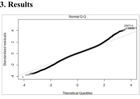
Figure 5. Normality Q-Q plot.

plot, as shown in Figure 5. Ideally, if the dataset was normally distributed, the graphed points would follow the slanted, dotted line across the plot, yet the tail ends of the plotted points stray from the ideal line, indicating a non-normal distribution. However, the sampling distribution of the coefficients is still considered to be normally distributed due to the central limit theorem, which suggests a large sample with random variables approaches normality regardless of the shape of the population distribution [29].

Next, multicollinearity was tested amongst the independent variables to determine if any of the variables were dependent upon each other. The variation inflation factor (VIF) was determined for each variable. An ideal VIF for a variable would be 1; however, VIFs under 10 are acceptable [28]. From the full model, two variables had a VIF above 10. Climate classification had a VIF of 37.64 while altitude had a VIF of 12.49. First, altitude was removed from the model which drastically changed the VIF for climate classification. It decreased the VIF from 37.64 to 4.20 indicating that altitude and climate classification were highly correlated. Besides this dramatic change, no other VIF values changed by more than 0.08. After the removal of altitude, the next highest VIF was temperature with a value of 4.41. Climate classification was also removed, and altitude was reinserted into the model to identify its effect. It also lowered all variables’ VIFs under 10, with temperature having the highest VIF of 3.69. Due to climate classification being the investigated variable within this research, altitude was ultimately selected to remain out of the model.

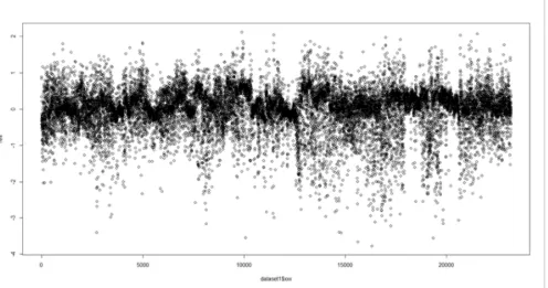
After multicollinearity, serial correlation was tested. To

test this assumption the data was first organized alphabetically by each location and then within each location the data was organized chronologically. Finally, a plot of the residuals was created, as shown in Figure 6 below. From this graph, autocorrelation can be clearly identified by the tendency of the data to continually stay above or below the x-axis at y = 0, labeled by the red line. Due to this evident trend, it was concluded that the residuals were correlated, which was further verified with the data failing a Durbin-Watson test [28]. Serial correlation was accounted for by using robust standard errors thus allowing for valid statistical inference. This process was completed in RStudio utilizing the package “sandwich” and command “coeftest” [30].

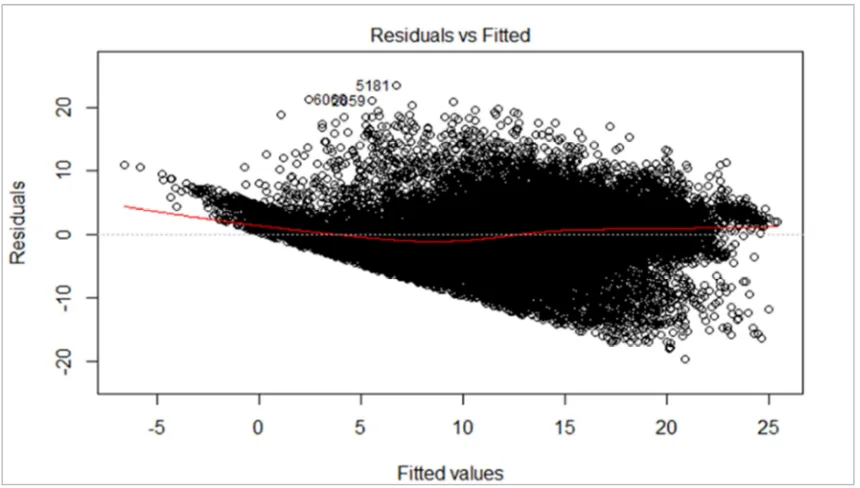
Following correlation, homoscedasticity of the residuals was tested by first looking at a plot of the residuals versus the fitted values of the model, as shown in Figure 7. In the plot, the values are at first closely grouped to one another, but progressively spread further apart moving left to right across the plot. This plot is depictive of heteroscedasticity. For homoscedasticity the values would ideally follow a random pattern with no specific clustering throughout the plot. Heteroscedasticity was confirmed with a Breusch-Pagan test [28]. Like serial correlation, heteroscedasticity was dealt with by using robust standard errors to adjust the standard error of the estimated coefficients within the model to determine the correct p-value and its significance. The robust standard errors were again calculated in RStudio utilizing the package “sandwich” and command “coeftest,” but specifying within the command to correct for both serial correlation and heteroscedasticity [30].

Figure 7. Residuals vs Fitted Values of Modified Model.

Finally, each variable’s significance was determined based upon a t-test using an alpha of 0.05 to determine the associated p-value’s significance [29]. Any p-value lower than 0.05 would result in a significant variable. After implementing robust standard errors, climate classification variables and Month 11 had the largest change in p-value. Of the climate classification variables, the p-value of Csa increased the most making the variable become more insignificant. This insignificance led to the conclusion that there is no difference on the effect of power production between Csa and the Af (the base climate of the model). The locations recorded with the climate classification Csa are both located in California while the location recorded with the climate classification Af is in Hawaii. The insignificance can potentially be explained by the two climates sharing similarities in local weather patterns and other climatic features while controlling for temperature, humidity and cloud ceiling. Similarly, Dfa and Csb also became insignificant after adjusting the standard errors for serial correlation and heteroscedasticity. Again, there could be similarities between these climates and Af, such as precipitation or wind speed, while controlling for temperature, humidity, and cloud ceiling. These variables were not removed from the model in order to maximize the number of locations the model can be applied to. In conclusion, the climates Csa, Dfa, and Csb could not be differentiated against Af in predicting the power output of horizontal photovoltaic panels.

The only other variable within the model that was insignificant was Month 11 (November) with a p-value of 390. This higher p-value could be due to November having a similar effect on horizontal photovoltaic power prediction when compared to the base month of the model (January) while controlling for the other variables in the model. This similar effect is most likely the position of the sun (solar

elevation) in the sky throughout the month. In summary, the effect on power production could not be distinguished between November and January. However, November was retained as it is a key variable that will be used for prediction.

In conclusion, the data obtained from the different test locations was developed into a simplified linear horizontal photovoltaic power model. The model was unable to meet the correlation and homoscedasticity assumptions, requiring a robust calculation of each coefficient’s standard error and p-value. Overall, the Köppen-Geiger climate classification that was determined to have the highest positive effect on horizontal photovoltaic power production compared to Af, is Cfb or warm temperate, fully humid, and warm summer.

With the completion of an initial model, two reduced models were compared against the full model to determine if climate classification and the weather variables temperature, humidity and cloud ceiling added value to the model. This analysis was conducted using a Wald test in order to properly account for the model’s robust standard errors. These errors were due to the model exhibiting heteroscedasticity and serial correlation. Both robust Wald tests were completed with the null hypothesis stating that the removed variables in the reduced models did not add value to the model [28]. In both instances, the test concluded with the rejection of the null hypothesis. In conclusion, it was determined that the Köppen-Geiger climates and the weather variables, temperate, humidity and cloud ceiling added value to the full model.

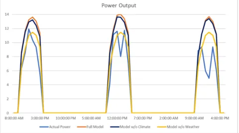
output of horizontal photovoltaic cells compared to the model with climate variables and no weather variables from the dataset. Although the weather variables have a better fit, incorporating climate did increase the amount of variation the model can explain by 3.05%. An example of each model’s goodness-of-fit can be seen in Figure 8 below. In the figure, the predicted power output is graphed against the actual power recorded at March Air Reserve Base between Nov 28 and Nov 30, 2017. Due to the time of day of the model being between 10:00AM and 3:00PM, times outside this period

were all represented as 0 W.

Table 3. Model Measures of Fit.

Model Type R-Squared Adjusted R-Squared

Full Model 0.5472 0.5468

Reduced Model without

Weather 0.3028 0.3021

Reduced Model without

Climate 0.5201 0.5196

Figure 8. Model Predictive Power Output.

Finally, a comparison was conducted of the predictive abilities of the full and reduced models. This was completed by inputting the validation dataset into each model and measuring the difference between the actual values recorded and the predictive values produced from the models. Root mean squared error and mean absolute error were used to compare the models. Running the 1,000 validation points through the models produced the values in Table 4. The results are similar to the R-squared values in Table 3 above, showing that the reduced model with weather variables but no climate variables produced less error while predicting horizontal photovoltaic power. However, when climate variables were included—i.e. the full model—the error decreased further. In conclusion, weather variables within the model were able to fit the validation data better while producing less error compared to climate variables.

Table 4. Model Measures of Prediction.

Model Type RMSE MAE

Full Model 4.614 3.534

Reduced Model without Weather 5.732 4.656

Reduced Model without Climate 4.749 3.620

4. Conclusion

Horizontal panel power output and weather data was collected from 28 test locations around the globe between June 2017 and September 2018. The model started with over a half billion data points collected from 16 reliable sites. However, the data was narrowed down to 14 test sites resulting in 24,179 usable data points, leading to the development of a linear model to predict power output. The model incorporated site-specific weather and geographical characteristics, along with Köppen-Geiger climate classifications in order to determine the effect of adding climate to the model. After performing a Wald test between the full model and reduced model without Köppen-Geiger climate variables, it was determined that the climate variables did provide added value to the full model. Although adding Köppen-Geiger variables provided added value to the model, these variables were less effective in fitting and predicting the validation dataset.

predictive abilities, it was concluded that cloud ceiling, temperature, and humidity were, on average, able to account for more variation compared to Köppen-Geiger climates. However, adding climate to these weather variables further increased the amount of variation explained by 3% and lowered the overall error within the model. The best Köppen-Geiger climate classification was Cfb, which was able to produce, on average, 30% more power compared to the climate Af. Similarly, the worst climate was BSk, which produced, on average, 9% less power compared to climate Af. Overall, the model can predict the power output of horizontal poly-crystalline photovoltaic panels at 1,213 DoD installations between the hours of 1000-1500. However, the final model was only able to account for approximately 55% of the variation within the data. In conclusion, it was discovered that the cost-effectiveness of a photovoltaic array depends on Köppen-Geiger climate regions, in addition to weather characteristics and the orientation of the array.

Authors’ Note: The views and opinions of authors

expressed herein do not necessarily state or reflect those of the United States Government or any agency thereof. Reference to specific commercial products does not constitute or imply its endorsement, recommendation, or favoring by the United States Government. The authors declare this is a work of the United States Government and is not subject to copyright protection within the United States. This article was cleared with case number 88ABW-2019-1585. Additionally, the authors thank Jada Williams for assistance with manuscript preparation.

References

[1] U. Kumar, K. Soon, M. Seyedmahmoudian, and S. Mekhilef, “Forecasting of photovoltaic power generation and model optimization : A review,” Renew. Sustain. Energy Rev., vol. 81, no. June 2017, pp. 912–928, 2018.

[2] J. A. Vásquez, K. Brecl, and M. Topič, “Köppen -Geiger-Photovoltaic Climate Classification,” 7th World Conf. Photovolt. Energy Convers. Kona, Hawaii, 2018.

[3] J. H. Nussbaum, “Analyzing the Viability of Photovoltaic Pavement Systems: A Study In Structural Testing Methods, Measuring Potential Power, and Quantifying the Risks of Implementation,” Air Force Institute of Technology, 2017. [4] C. J. Booker, “Analysis of Temperature and Humidity Effects

on Horizontal Photovoltaic Panels,” Air Force Institute of Technology, 2018.

[5] J. A. Applebee, “Determining the Viability and Efficiency of GP3L Photovoltaic System Study At Air Force Installations in Various Climate Regions Air Force Institute of Technology,” Air Force Institute of Technology, 2018.

[6] M. Belda, E. Holtanová, T. Halenka, and J. Kalvová, “Climate classification revisited: From Köppen to Trewartha,” Clim. Res., vol. 59, no. 1, pp. 1–13, 2014.

[7] M. Kottek, J. Grieser, C. Beck, B. Rudolf, and F. Rubel, “World map of the Köppen-Geiger climate classification

updated,” Meteorol. Zeitschrift, vol. 15, no. 3, pp. 259–263, 2006.

[8] C. Beck, J. Grieser, M. Kottek, F. Rubel, and B. Rudolf, “Characterizing global climate change by means of Koeppen climate classification,” Clim. Status Rep. 2005, p. 10, 2006. [9] D. C. Jordan, J. H. Wohlgemuth, and S. R. Kurtz, “Technology

and climate trends in PV module degradation,” 27th Eur. Photovolt. Sol. Energy Conf. Exhib., pp. 3118–3124, 2012.

[10] I. Mahlstein, J. S. Daniel, and S. Solomon, “Pace of shifts in climate regions increases with global temperature,” Nat. Clim. Chang., vol. 3, no. 8, pp. 739–743, 2013.

[11] F. P. Tso, D. R. White, S. Jouet, J. Singer, and D. P. Pezaros, “The Glasgow raspberry Pi cloud: A scale model for cloud computing infrastructures,” Proc. - Int. Conf. Distrib. Comput. Syst., pp. 108–112, 2013.

[12] V. Vujovic, V. Vujović, and M. Maksimović, “Raspberry Pi as a Wireless Sensor node : Performances and constraints Raspberry Pi as a Wireless Sensor Node : Performances and Constraints,” 2014 37th Int. Conv. Inf. Commun. Technol. Electron. Microelectron. MIPRO 2014 - Proc., pp. 26–30, 2014.

[13] Y. Sharon, B. Khachatryan, and D. Cheskis, “Low current Hall Effect Sensor,” 2018.

[14] NOAA, “National Oceanic and Atmospheric Administration.”. [15] M. A. Green, K. Emery, Y. Hishikawa, W. Warta, and E. D. Dunlop, “Solar cell efficiency tables (version 43),” Prog. Photovoltaics Res. Appllications, vol. 22, pp. 1–9, 2015.

[16] National Optical Astronomy Observatory, “Recommended Light Levels (Illuminance) for Outdoor and Indoor Venues.”. [17] A. Ã. Virtuani, E. Lotter, and M. Powalla, “Influence of the

light source on the low-irradiance performance of Cu (In, Ga) Se 2 solar cells,” vol. 90, pp. 2141–2149, 2006.

[18] O. Zogou, “Experimental and computational investigation of the thermal and electrical performance of a new building integrated photovoltaic concept,” 2011.

[19] E. Skoplaki and J. A. Palyvos, “On the temperature dependence of photovoltaic module electrical performance: A review of efficiency/power correlations,” Sol. Energy, vol. 83, no. 5, pp. 614–624, 2009.

[20] M. M. Fouad, L. A. Shihata, and E. S. I. Morgan, “An integrated review of factors influencing the performance of photovoltaic panels,” Renew. Sustain. Energy Rev., vol. 80, pp. 1499–1511, 2017.

[21] F. H. Gandoman, S. H. E. Abdel, N. Omar, A. Ahmadi, and F. Q. Alenezi, “Short-term solar power forecasting considering cloud coverage and ambient temperature variation effects,” Renew. Energy, vol. 123, pp. 793–805, 2018.

[22] C. J. Smith, J. M. Bright, and R. Crook, “Cloud cover effect of clear-sky index distributions and differences between human and automatic cloud observations,” Sol. Energy, vol. 144, pp. 10–21, 2017.

[24] J. Antonanzas, R. Urraca, F. J. Martinez-de-Pison, and F. Antonanzas, “Optimal solar tracking strategy to increase irradiance in the plane of array under cloudy conditions: A study across Europe,” Sol. Energy, vol. 163, pp. 122–130, 2018.

[25] D. King, W. Boyson, and J. Kratochvil, “Analysis of factors influencing the annual energy production of photovoltaic systems,” in Photovoltaic Specialists, IEEE Conference, 2002, pp. 1356–1361.

[26] A. J. Gutiérrez-trashorras, E. Villicaña-ortiz, E. Álvarez-álvarez, J. M. González-caballín, J. Xiberta-bernat, and M. J. Suarez-lópez, “Attenuation processes of solar radiation. Application to the quantification of direct and diffuse solar irradiances on horizontal surfaces in Mexico by means of an

overall atmospheric transmittance,” Renew. Sustain. Energy Rev., vol. 81, pp. 93–106, 2018.

[27] A. Nagengast, C. Hendrickson, and H. Scott Matthews, “Variations in photovoltaic performance due to climate and low-slope roof choice,” Energy Build., vol. 64, pp. 493–502, 2013.

[28] M. Kutner, C. Hachtsheim, J. Neter, and W. Li, Applied Linear Statistical Models, 5th ed. McGraw-Hill Irwin, 2005.

[29] J. McClave, P. Benson, and T. Sincich, Statistics for Business and Economics, 12th ed. Pearson, 2014.