Article
A High Performance Computing Implementation of
Iterative Random Forest for the Creation of Predictive
Expression Networks
Ashley Cliff1,2, Jonathon Romero1,2, David Kainer2, and Daniel Jacobson1,2*
1 Bredesen Center for Interdisciplinary Research and Graduate Education, University of Tennessee Knoxville 2 Oak Ridge National Laboratory
* Correspondence: [email protected]
Abstract: As time progresses and technology improves, biological data sets are continuously increasing in size. New methods and new implementations of existing methods are needed to keep
pace with this increase. In this paper, we present a high performance computing(HPC)-capable
implementation of Iterative Random Forest (iRF). This new implementation enables the
explainable-AI eQTL analysis of SNP sets with over a million SNPs. Using this implementation we also present a new method, iRF Leave One Out Prediction (iRF-LOOP), for the creation of Predictive
Expression Networks on the order of 40,000 genes or more. We compare the new implementation
of iRF with the previous R version and analyze its time to completion on two of the world’s
fastest supercomputers Summit and Titan. We also show iRF-LOOP’s ability to capture biologically
significant results when creating Predictive Expression N etworks. This new implementation of iRF will enable the analysis of biological data sets at scales that were previously not possible.
Keywords: Random Forest; Iterative Random Forest; gene expression networks; high performance
computing; X-AI-based eQTL
1. Introduction
Due to innovation in the areas of genome sequencing and ’omics analysis, biological data is entering the age of big data. As opposed to other fields of research, biological data sets tend to have large feature quantity, but much smaller sample counts, such as in a GWAS population where there are typically hundreds to thousands of genotypes, but millions of SNPs. The number of independent features of biological systems is large, and would require many lifetimes of the entire
scientific community to sufficiently study[1]. The ability to determine which features are influential
to a particular phenotype, be it SNPs, gene expression, or interactions between multiple molecular pathways, is essential in reducing the full feature space to a subset that is feasible to analyze.
Many methods exist to determine feature importance and feature selection, such as Pearson
Correlation, Mutual Information (MI), Sequential Feature Selection (SFS)[2], Lasso, and Ridge
Regression. Random Forest[3] is a commonly used machine learning method for making predictions,
and while not classically defined as a feature selection method, it is useful in scoring feature importance. During the training phase, decision trees are built, where a subset of features is examined at each decision point and the one that best divides the data is chosen. Feature importances are calculated for each feature based on its location and effectiveness within the tree structures. By using random subsets of the training data for each tree and considering random features for each decision point, Random Forest prevents over fitting. Because of the nature of decision trees, the importance of any chosen feature is inherently conditional on the features that were chosen previously. In this way the Random Forest is able to account for some of the interconnected dependencies that occur in biological
systems. As a non-linear model, Random Forest has been applied to a range of biological data problems,
including GWAS, genomic prediction, gene expression networks and SNP imputation[4].
Iterative Random Forest[5] (iRF) is an algorithmic advancement of Random Forest (RF), which
takes advantage of Random Forests ability to produce feature importance and produces a more accurate model by iteratively creating weighted forests. In each iteration, the importance scores from the previous iteration are used to weight features for the current forest. Until now, iRF was
implemented solely as an R package[6]. While useful for small projects, it was not designed for big data
analysis. This paper describes the process of implementing a high performance computing enabled
iRF, using MPI (Message Passing Interface)[7]. This new implementation enabled the creation of
Predictive Gene Expression Networks with 40,000 genes and quickly completed the feature importance
calculations for 1.7 millionArabidopsis thalianaSNPs in relation to a gene expression profile, as part of a
genome-wide explainable-AI-based eQTL analysis.
2. Materials and Methods
2.1. Random Forest and Iterative Random Forest Methods
The base learner for the Random Forest (RF) and Iterative Random Forest (iRF) methods is the decision tree, also known as a binary tree. A decision tree starts with a set of data: samples, features, and a dependent variable. The goal is to divide the samples, through decisions based on the features, into subsets containing homogeneous dependent variable values, generally following the
CART (Classification and Regression Trees) method[8], where each decision divides one node into two
child nodes. This is a greedy algorithm which will continue to divide the samples into child nodes, based on a scoring criteria, until a stopping criteria is met. Decision trees are weak learners and tend to over-fit to the data provided.
A Random Forest is an ensemble of decision trees. However, the trees in a Random Forest differ from standard decision trees in that each tree starts with a subset of the samples, chosen via random sampling with replacement. Also differing from standard decision trees, the features being considered at each node are a random subset, with the number of features provided by a parameter. Once a forest has been generated, the importance of each feature can be calculated from node impurity, such as the Gini index for classification or variance explained for regression, or permutation importance. Unlike a single decision tree, a Random Forest is a strong learner, because it averages many weak learners and avoids putting too much weight on outlier decisions. The number of trees in a forest is a parameter that is chosen by the user and has an effect on the accuracy of the model.
Iterative Random Forest expands on the Random Forest method by adding an iterative boosting process, producing a similar effect to Lasso in a linear model framework. First, a Random Forest is created where features are unweighted and have an equal chance of being randomly sampled at any given node. The resulting importance scores for the features are then used to weight the features in the next forest, thus increasing the chance that important features are evaluated at any given node.
This process of weighting and creating a new Random Forest is repeateditimes, whereiis set by the
user. Due to the ability to easily follow the decisions that these models make, they have been deemed
explainable-AI (X-AI)[1], which differs from many standard machine and deep learning methods.
The number of iterations allows the user to find a balance between over- and under-parameterization of the model, by progressively eliminating features.
2.2. Implementation of iRF in C++
We used Ranger[9], an open source Random Forest implementation in C++, as the core of
our iRF implementation. Ranger already implements the decision tree and forest creation aspects, but implements neither the communication necessary for running on multiple compute nodes of a distributed HPC system, nor the iterative aspect of iRF.
Within our implementation, each decision tree is initialized with a random subset of the data sample vectors and is then built in an independent process. Groups of trees (sub-forests) are built on compute nodes and then sent to a master compute node that aggregates them into a full Random Forest. This is done by giving each sub-forest a randomly generated seed number which determines the random subset of data each tree in a sub-forest uses, allowing for a higher likelihood of unique random data subsets on each tree. Once in the form of a single Random Forest, Ranger’s functions for forest analysis are used, including feature importance aggregation.
On a distributed system, where parts of the forest are created on different compute nodes, the aggregation of results requires the majority of the inter-node communication. This process relies on MPI (the Message Passing Interface), an internode-communication standard for parallel programming,
and Open-MPI[10], an open source C library containing functions that follow the MPI standard.
To implementiiterations, the forest creation and aggregation is performeditimes. After the
completion of each iteration, the feature weights are written to a file. At the beginning of the next iteration, this file is read into an array that is used to create the weighted distribution from which features are sampled during the decision process at each node on each tree. This process, while potentially slow due to the file I/O, uses the preexisting functionality of weighted sampling from Ranger.
2.3. iRF-LOOP: iRF Leave One Out Prediction
Given a data set ofnfeatures andmsamples, iRF Leave One Out Prediction (iRF-LOOP) starts
by treating one feature as the dependent variable (Y) and the remainingn-1 features as predictor
matrix (X) of sizem x n-1. Using an iRF model, the importance of each feature in X, for predicting
Y, is calculated. The result is a vector, of sizen, of importance scores (the importance score of Y, for
predicting itself, has been set to zero). This process is repeated for each of thenfeatures, requiringn
iRF runs. Thenvectors of importance scores are concatenated into ann x nimportance matrix. To keep
importance scores on the same scale across the importance matrix, each column is normalized relative to the sum of the column. The normalized importance matrix can be viewed as a directional adjacency
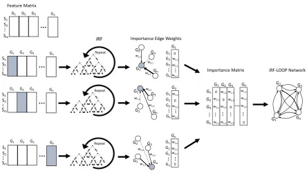
matrix, where values are edge weights between features. See figure1for a diagram of this process.
Due to the nature of iRF, the adjacency matrix is not symmetric as feature A may predict feature B with a different importance than feature B predicts feature A.
2.4. Big Data: Showing the scale of iRF with Arabidopsis thaliana SNP Data
A typical use case of iRF, with a matrix of features and a single target vector of outcomes, becomes comparable to an X-AI-based eQTL analysis, when the matrix of features is a set of single nucleotide polymorphisms (SNPs) and the dependent variable vector is a gene’s expression measured across samples. This analysis determines which set(s) of SNPs are important to variation in the gene’s expression.
We obtainedArabidopsis thalianaSNP data from the Weigel laboratory at the Max Planck Institute
for Developmental Biology, available at https://1001genomes.org/data/GMI-MPI/releases/v3.1/.
We filtered the SNPs using bcftools 1.9[11] to keep only those that were biallelic, had a minor allele
…
G1 G2 G3 Gn
S1 S2 Sm … Feature Matrix
…
Gn S1 S2 Sm……
Gn S1 S2 Sm……
Gn S1 S2 Sm… Repeat Repeat Repeat iRF G1 G2 G3 Gn G1 G2 G 3 Gn Importance Edge WeightsG1 G2 G3 Gn G1 G2 G3 Gn iRF-LOOP Network G1 G2 G3 … w2,1 w3,1 wn,1 … Gn G1 0
G1G2G3 Gn G1 G2 G3 Gn …
…
0 0 0 0 G2 G2 G3 … w1,2 w3,2 wn,2 … Gn G1 0 Gn G2 G3 … w1,n w3,n … Gn G1 w2,n 0 w2,1 w3,1 wn,1 w1,2 w3,2 wn,2 w1,n w2,n w3,n w2,1 w3,1 wn,1 w1,2 w3,2 wn,2 … … w1,n w2,n w3,n … … w1,3 w2,3 wn,3 Importance MatrixG1 G2 G3
G1 G2 G3
G1 G2 G3
Figure 1. The diagram shows the process of iRF-LOOP for a set of Expression profiles, creating a Predictive Expression Network. Each gene is independently treated as the target for an iRF run, with all other genes as predictors. iRF provides importance scores of each predictor gene, and creates network edge weights between target and predictors. These importance scores are then combined into an edge matrix, providing a value for each possible connection, from which a network can be generated. Generally, the weights are thresholded at some value, determined through other means, and only edges with large enough weights are included in the final network. Due to the inherent directionality of a prediction, the edges are weighted, and not likely to be symmetric.
We obtainedArabidopsis thalianaexpression data[12] from 727 samples and 24175 genes. Of these
727 samples, 666 samples were also present in the SNP data set. The vector of gene expression values for gene AT1G01010 for those 666 samples was used as the dependent variable for iRF. The feature set was the full set of 1.71 million SNPs, for the same 666 samples. While this is not a large number of samples, this is clearly a large number of features.
The C++ iRF code was run using these data as input with five iterations, each generating a forest containing 1000 trees. The number of trees was chosen as a value close to the square root of the number of features (a common setting for this parameter), where each feature has a 95% chance of being included in the feature subset within the first two layers in at least one tree. This helps to guarantee that all features are considered at least once across an iteration. HPC node quantities of 1, 2, 5, and 10 were used to show run time changes as the amount of resources increases.
Due to the large number of SNPs, the full data could not fit in memory on a standard laptop, for use in the R iRF program. Instead, small subsets of features of sizes 2,000, 1,000, 500, 100 and 50 features were run, each using the full 666 samples and the same AT1G01010 gene expression dependent variable. Each feature set was run three times and averaged to account for the inherent stochasticity in the algorithm. Only one run was performed for each parameter set on Summit with the full data set due to limited compute time availability.
2.5. Using iRF-LOOP to Create Predictive Expression Networks
Given a matrix of gene expression data, there are a multitude of approaches for inferring which genes potentially regulate the expression of other genes, ranging in complexity from pairwise Pearson
(DBNs)[15]. Due to the large number of features and the complexity of the interactions between them, Random Forest-type approaches are well suited to this task.
We applied iRF-LOOP to a matrix of gene expression data measured in 41,335 genes across 720
genotypes ofPopulus trichocarpa(Black cottonwood). The RNAseq data [16] from were obtained from
the NCBI SRA database (SRA numbers: SRP097016– SRP097036; www.ncbi.nlm.nih.gov/sra). Reads
were aligned to thePopulus trichocarpav.3.0 reference[17]. Transcript per million (TPM) counts were
then obtained for each genotype, resulting in a genotype- transcript matrix, as referenced in [18]. The
adjacency matrix resulting from iRF-LOOP represents a Predictive Expression Network (PEN) where a directed edge (AB) between and two genes (A and B) is weighted according to the importance of gene A’s expression in predicting gene B’s expression, conditional on all other genes in the iRF model. We removed zeros and produced four thresholded networks, keeping the top 10%, 5%, 1%, and 0.1% of edges respectively.
To determine the biological significance of the PEN produced by the iRF-LOOP, we compared each of the four thresholded networks to a network of known biological function, created from Gene Ontology (GO) annotations. GO is a standardized hierarchy of gene descriptions that captures the current knowledge of gene function. It is accepted that there is both missing information and some error, nevertheless it is useful as a broad truth set for large sets of genes. We calculated scores for each network by intersecting with the GO network. We then evaluated the probability of achieving such scores relative to random chance by creating null distributions of scores produced by random permutation of the iRF-LOOP networks and calculated t-statistics for each threshold.
We created a Populus trichocarpa GO network for the Biological Process (BP) GO terms, using
annotations from [19]. Genes are connected if they share one or more GO terms. The edge weight
between two genes equals 1
sum(1...n−1), wherenis the number of genes with the shared term. If
two genes share more than one GO term, then the largest weight is used for the edge. In this way, if two genes share a broad GO term (a less specific function), the value of their connection weight is low. Conversely, two genes that share a rare GO term (highly specific function) have a higher edge weight. To avoid edges between very loosely associated genes, only GO terms with less than 1000 genes were used for this analysis. The resulting network provides the relationship between genes that share some level of known functionality.
To generate the null distribution of intersect scores for each thresholded PEN, the node labels of each network were randomly permuted 1000 times, and each random network was scored against the GO network. From these null distributions, t-statistics were calculated for the score of each thresholded Predictive Expression Network.
2.6. Comparison of R to C++ Code
To compare the original iRF R code to the new implementation, both were run on a single node of Summit with a variety of running parameters. These parameters included all combinations of 100, 1000, and 5000 trees and 1, 2, 3, and 4 threads for 1000 features. All combinations were run three times
and the scores were averaged. Due to the R code’s doParallel[20] back-end not being designed for a
HPC system, the R code was limited to a single CPU on a node with up to four independent threads.
For consistency, the new implementation was limited to the same resources. A subset of thePopulus
trichocarpaexpression data mentioned above was used as the feature set.
2.7. Computational Resources
processor and 32 GB of DDR3 ECC memory. The 2015 Macbook Pro has a 3.1 Ghz Intel Core i7 Processor and 16 GB of DDR3 memory.
3. Results
3.1. Comparison of the R to C++ Code
Previously, the only published iRF code existed as an R library. This library uses R’s ’doParallel’ functionality, generally allowing for multi-core thread parallelism on shared memory CPUs. However, this system did not function on Summit, so our analysis was limited to running differences on a single Summit CPU.
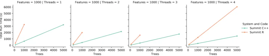
Figure 2.Each of these graphs shows the total run time as the number of threads increases. Both the R code and C++ code were run on Summit. Note for 5000 trees, the R implementation failed to complete using less than 4 threads.
To compare the R code to the C++ code, both programs were run on a single CPU on Summit. While this is a small resource set, it was sufficient in showing trends and making comparisons between
the two implementations. Figure2shows the the time to completion as the number of threads increases.
As the number of threads that the runs are spread over increases, both implementations decrease in run time. However, for the 5000 tree runs for 1, 2, and 3 threads the R code was unable to complete in the 2 hour time limit set by the Summit system. This is a good indication that these runs were not
efficient enough, as the C++ implementation runs were able to complete. Similarly, as seen in figure3,
as the number of trees increases, the R code takes significantly longer than the C++ code to complete. Together, these figures show that in a one-on-one comparison using appropriate resources, the C++ implementation is more efficient than the R implementation, and is able to handle more computations per unit of time.
3.2. Scaling Results for Big Data: Arabidopsis thaliana SNPs to Gene Expression
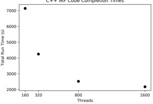
To show how well our implementation of iRF handles large feature sets, a set of 1.7 million SNPs fromArabidopsis thalianawas used to predict the expression of gene AT1G01010. Figure4shows the times to completion for the four thread quantities tested on Summit (160 threads per compute node). Our implementation was easily able to handle the data set for all thread quantities and finished in reasonable amounts of time. It is worth noting that there were diminishing returns as the number of nodes gets close to 10 (1600 threads) since the number of trees per node at this scale would only be 100 (1000 trees total spread over 10 nodes) and did not utilize the resources to its fullest potential. For a larger feature set, a larger number of trees would be advised, and a larger number of nodes could be utilized more efficiently.
Figure 4.The graph shows the run times for four different compute node quantities, each completing 1000 trees for the 1.7 million SNPs.
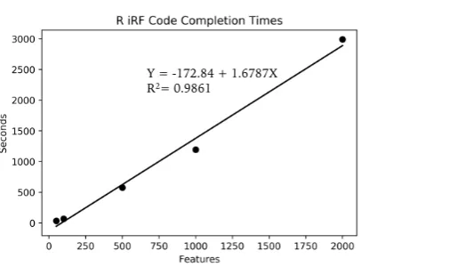
To try to determine approximately how long this calculation would take on a standard laptop,
multiple smaller runs were completed. Figure5shows the run times for multiple feature amounts for
the R iRF code on one cpu of a 2015 MacBook Pro laptop. The linear fit, while not perfect, is accurate enough for a rough estimate for larger feature sizes. Using the provided equation, the 1.7 million feature set run on Summit would take approximately 33 days to complete on a laptop, given that the system had enough memory to contain the data set and results, which most standard laptops do not have. When compared to the approximately 40 minutes required on 5 nodes of Summit, it is easy to see what a difference these resources, and programs that can utilize them, can make.
3.3. Predictive Expression Networks
We used iRF-LOOP to produce Predictive Expression Networks forPopulus trichocarpa. Figure6(a)
shows the run time results for the C++ code for all varying numbers of threads and trees, for one of the
approximately 40,000 iRF runs within an iRF-LOOP. Figure6(b) shows the total run time as the number
of threads increases on Summit and Titan for the C++ code, showing that iRF works comparably on different system architectures. Due to the architecture differences, Summit nodes can independently run 160 threads simultaneously while Titan nodes could only do 16 threads. Summit (in red) had a harder time with larger data on a single thread, but both systems function well as the number of threads increases to appropriate numbers for general uses cases. The full graph of all parameters comparing time to completion on Summit and Titan is available in figure S1.
Table1shows the number of edges and nodes in the four resulting thresholded PENs. The GO
network that was generated to analyse the PENs contained 16,836 nodes and 3,274,574 edges. Figure7
Y = -172.84 + 1.6787X R2= 0.9861
Figure 5.The graph shows the run time for five different feature sizes, on a single CPU of a standard MacBook Pro laptop. Each point represents the average of three runs. A linear regression was fit, with the equation shown. The fit is not perfect, but is enough to indicate that the run time increase approximately linearly in comparison to the number of features.
(a) (b)
Figure 6.Graph (a) provides the total run time for the C++ code on Summit, with various tree and thread counts, for 40,000 features. Graph (b) provides a comparison of the C++ code on Summit and Titan, two HPC systems. For both graphs, run time is in seconds.
Network Nodes Edges Intersect Score Null Dist Mean Null Dist s.d. t-statistic
0.1% PEN 26,617 57,112 59.74 0.9831 0.2597 226.27
1% PEN 38,758 563,887 213.28 9.6930 0.8720 233.47
5% PEN 39,349 2,795,636 484.07 48.1309 2.0784 209.74
10% PEN 39,349 5,846,200 692.08 100.5038 2.9316 201.79
Table 1.The table provides the graph results for the 4 thresholded Predictive Expression Networks. The listed mean and standard deviation are for the corresponding null distributions, as pictured in figure8. The p-values for the listed t-statistics were effectively zero.
Also shown in table1are the mean and standard deviation for the null distribution of the random
permutations for each thresholded PEN. The null distribution and intersect score (in red) for two
of the four networks are shown in figure8. The other two null distributions are available in figure
null distributions are provided in figure S3, showing that the null distributions are all close enough to normal.
A
B
C
D
E
F
G
H
ribosomal large subunit assembly ribosomal small subunit assembly
maturation of LSU-rRNA Gene Ontology Associations
Gene Node Labels
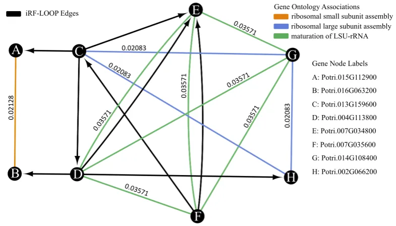
A: Potri.015G112900 B: Potri.016G063200 C: Potri.013G159600 D: Potri.004G113800 E: Potri.007G034800 F: Potri.007G035600 G: Potri.014G108400 H: Potri.002G066200
0.
02128
0.02083
0.
03571
0.03571
0.03571
0.
02083
0.03571
0.03571
0.03571 0.02083
iRF-LOOP Edges
Figure 7.The network shown is a small example from the iRF prediction expression network overlayed with the GO process network. The nodes represent the genes. The black edges represent the iRF edges, which are directedfromthe featuretothe predicted target. The colored edges represent different GO associations between genes, meaning that they share a GO term. Using the provided GO edge weights, this network has an intersect score of 0.0714, from connections DE and FE having both iRF edges and GO edge
(a) (b)
Figure 8.Graph (a) shows the null distribution histogram (blue) and the iRF network score (red) for the top 10 percent of edges. Graph (b) shows the null distribution histogram (blue) and the iRF network score (red) for the top 0.1 percent of edges. Note that the x-axis is different for the two graphs. Each distribution was calculated from 1000 random permutations.
4. Discussion
We have presented a high performance computing-capable implementation of Iterative Random Forest. This implementation uses Ranger, C++, and MPI to utilize the resources available on multi-node computation resources. We have shown that our implementation can perform X-AI based eQTL-type analyses with millions of SNPs and have shown its ability to scale with multiple parameters. Using iRF
took approximately the same time as the shown above, would take approximately 705 days using 5 nodes, or 84,680 compute node hours, or 18 hours using 4,600 Summit nodes. To complete the analysis for all 24,175 gene expression predictions on a laptop using the R code would take approximately 2,191 years. While this comparison seems impressive, it should also be noted that for a larger feature set and larger number of trees the large resources will be even more appropriate as the scaling factor will be even less effected by overhead. For cases where the number of SNPs is 10 million and higher, the code should be even more efficient on HPC systems. However, as not everyone has access to the fastest computers in the world this code could still run efficiently on a smaller system using a smaller set of SNPs.
Using this new implementation, we developed iRF-LOOP and used it to produce Predictive Expression Networks which were shown to have biologically relevant information. The process of iRF-LOOP has the potential to be used for a wide variety of data analysis problems. With an appropriate amount of compute resources, it would be possible to build connected networks for each level of ’omics data available for a given species. The same concept could also be used to connect ’omics layers to each other as shown by using the SNPs in the X-AI based eQTL analysis. This machine learning method is not limited to genetics or biology and has uses in other fields where systems can be represented as a matrix.
Downstream of any iRF analysis, there is the possibility of finding epistatic interactions among
features from the resulting forests, using Random Intersection Trees (RIT) [21]. This method works
regardless of the data type for the features, where it can find sets of SNPs that influence gene expression or sets of genes that influence other gene’s expression, adding another set of nodes and groups to a Predictive Expression Network.
5. Software Availability
The Ranger-based Iterative Random Forest code is available athttps://github.com/Jromero1208/
RangerBasediRF.
Supplementary Materials:The following are available online athttp://www.mdpi.com/2073-4425/xx/1/5/, Figure S1: Runtime on HPC Systems. , Figure S2: Null Distribution Plots, Figure S3: Quantile-Quantile Plots for the PENs.
Author Contributions:Conceptualization, A.C., D.J. and J.R.; methodology, A.C.; software, A.C.; validation, A.C.; formal analysis, A.C.; investigation, A.C.; resources, D.J.; data curation, A.C., J.R., and D.K.; writing—original draft preparation, A.C. and J.R.; writing—review and editing, A.C., J.R., D.K. and D.J.; visualization, A.C.; supervision, D.K. and D.J.; project administration, D.J.; funding acquisition, D.J.
Funding: Funding provided by the Plant-Microbe Interfaces Scientific Focus Area in the Genomic Science Program, The Center for Bioenergy Innovation (CBI). The U.S. Department of Energy Bioenergy Research Centers are supported by the Office of Biological and Environmental Research in the DOE Office of Science.
Acknowledgments: This research used resources of the Oak Ridge Leadership Computing Facility and the Compute and Data Environment for Science at Oak Ridge National Laboratory, which is supported by the Office of Science of the U.S. Department of Energy under Contract No. DE-AC05-00OR22725. The manuscript was coauthored by UT-Battelle, LLC under Contract No. DE-AC05-00OR22725 with the US Department of Energy. The US Government retains and the publisher, by accepting the article for publication, acknowledges that the US Government retains a nonexclusive, paid-up, irrevocable, worldwide license to publish or reproduce the published form of this manuscript, or allow others to do so, for US Government purposes. The Department of Energy will provide public access to these results of federally sponsored research in accordance with the DOE Public Access Plan (http://energy.gov/downloads/doe-public-access-plan).
Conflicts of Interest:The authors declare no conflict of interests.
Abbreviations
iRF Iterative Random Forest iRF-LOOP iRF Leave One Out Prediction
RF Random Forest
MPI The Message Passing Interface HPC High Performance Computing
GO Gene Ontology
SNP Single Nucleotide Polymorphism eQTL Expression Quantitative Trait Loci X-AI Explainable Artificial Intelligence RIT Random Intersection Trees
1. Harfouche, A.; Jacobson, D.; Kainer, D.; Romero, J.; Harfouche, A.H.; Scarascia Mugnozza, G.; Moshelion, M.; Tuskan, G.; Keurentjes, J.; Altman, A. Accelerating Climate Resilient Plant Breeding by Applying Next-Generation Artificial Intelligence.Trends in Biotechnology2019. Accepted and Selected for Cover. 2. Chandrashekar, G.; Sahin, F. A survey on feature selection methods. Computers Electrical Engineering2014,
40, 16.
3. Breiman, L. Random Forests. Machine Learning2001,45, 5–32. doi:10.1023/A:1010933404324.
4. Chen, X.; Ishwaran, H. Random forests for genomic data analysis. Genomics 2012, 99, 323–329. doi:10.1016/j.ygeno.2012.04.003.
5. Basu, S.; Kumbier, K.; Brown, J.B.; Yu, B. Iterative random forests to discover predictive and stable high-order interactions. Proceedings of the National Academy of Sciences 2018, 115, 1943–1948,
[https://www.pnas.org/content/115/8/1943.full.pdf]. doi:10.1073/pnas.1711236115. 6. Basu, S.; Kumbier, K.iRF: iterative Random Forests, 2017. R package version 2.0.0. 7. Walker, D.W.; Dongarra, J.J. MPI: a standard message passing interface.
8. Breiman, L.; Friedman, J.; Olshen, R.; Stone, C. Classification and Regression Trees1984.
9. Wright, M.; Ziegler, A. ranger: A Fast Implementation of Random Forests for High Dimensional Data in C++ and R.Journal of Statistical Software, Articles2017,77, 1–17. doi:10.18637/jss.v077.i01.
10. Gabriel, E.; Fagg, G.E.; Bosilca, G.; Angskun, T.; Dongarra, J.J.; Squyres, J.M.; Sahay, V.; Kambadur, P.; Barrett, B.; Lumsdaine, A.; Castain, R.H.; Daniel, D.J.; Graham, R.L.; Woodall, T.S. Open MPI: Goals, Concept, and Design of a Next Generation MPI Implementation. Proceedings, 11th European PVM/MPI Users’ Group Meeting; , 2004; pp. 97–104.
11. Li, H. A statistical framework for SNP calling, mutation discovery, association mapping and population genetical parameter estimation from sequencing data. Bioinformatics2011,27, 2987–2993. doi:10.1093/bioinformatics/btr509.
12. Kawakatsu, T.; Huang, S.S.C.; Jupe, F.; Sasaki, E.; Schmitz, R.J.; Urich, M.A.; Castanon, R.; Nery, J.R.; Barragan, C.; He, Y.; Chen, H.; Dubin, M.; Lee, C.R.; Wang, C.; Bemm, F.; Becker, C.; O’Neil, R.; O’Malley, R.C.; Quarless, D.X.; Consortium, .G.; Schork, N.J.; Weigel, D.; Nordborg, M.; Ecker, J.R. Epigenomic Diversity in a Global Collection of Arabidopsis thaliana Accessions.Cell2016,166, 492–505. doi:10.1016/j.cell.2016.06.044.
13. Margolin, A.A.; Nemenman, I.; Basso, K.; Wiggins, C.; Stolovitzky, G.; Favera, R.D.; Califano, A. ARACNE: An Algorithm for the Reconstruction of Gene Regulatory Networks in a Mammalian Cellular Context. BMC Bioinformatics2006,7, S7. doi:10.1186/1471-2105-7-S1-S7.
14. Huynh-Thu, V.A.; Irrthum, A.; Wehenkel, L.; Geurts, P. Inferring Regulatory Networks from Expression Data Using Tree-Based Methods. PLOS ONE2010,5, 1–10. doi:10.1371/journal.pone.0012776.
15. Perrin, B.E.; Ralaivola, L.; Mazurie, A.; Bottani, S.; Mallet, J.; d’Alché–Buc, F. Gene networks inference using dynamic Bayesian networks . Bioinformatics 2003, 19, ii138–ii148,
[http://oup.prod.sis.lan/bioinformatics/article-pdf/19/suppl_2/ii138/434708/btg1071.pdf]. doi:10.1093/bioinformatics/btg1071.
quantitative trait loci analyses reveal roles of HCT2 in caffeoylquinic acid biosynthesis and its regulation by defense-responsive transcription factors in Populus. New Phytologist2018,220, 502–516,
[https://nph.onlinelibrary.wiley.com/doi/pdf/10.1111/nph.15297]. doi:10.1111/nph.15297.
17. Tuskan, G.A.; DiFazio, S.; Jansson, S.; Bohlmann, J.; Grigoriev, I.; Hellsten, U.; Putnam, N.; Ralph, S.; Rombauts, S.; Salamov, A.; Schein, J.; Sterck, L.; Aerts, A.; Bhalerao, R.R.; Bhalerao, R.P.; Blaudez, D.; Boerjan, W.; Brun, A.; Brunner, A.; Busov, V.; Campbell, M.; Carlson, J.; Chalot, M.; Chapman, J.; Chen, G.L.; Cooper, D.; Coutinho, P.M.; Couturier, J.; Covert, S.; Cronk, Q.; Cunningham, R.; Davis, J.; Degroeve, S.; Déjardin, A.; dePamphilis, C.; Detter, J.; Dirks, B.; Dubchak, I.; Duplessis, S.; Ehlting, J.; Ellis, B.; Gendler, K.; Goodstein, D.; Gribskov, M.; Grimwood, J.; Groover, A.; Gunter, L.; Hamberger, B.; Heinze, B.; Helariutta, Y.; Henrissat, B.; Holligan, D.; Holt, R.; Huang, W.; Islam-Faridi, N.; Jones, S.; Jones-Rhoades, M.; Jorgensen, R.; Joshi, C.; Kangasjärvi, J.; Karlsson, J.; Kelleher, C.; Kirkpatrick, R.; Kirst, M.; Kohler, A.; Kalluri, U.; Larimer, F.; Leebens-Mack, J.; Leplé, J.C.; Locascio, P.; Lou, Y.; Lucas, S.; Martin, F.; Montanini, B.; Napoli, C.; Nelson, D.R.; Nelson, C.; Nieminen, K.; Nilsson, O.; Pereda, V.; Peter, G.; Philippe, R.; Pilate, G.; Poliakov, A.; Razumovskaya, J.; Richardson, P.; Rinaldi, C.; Ritland, K.; Rouzé, P.; Ryaboy, D.; Schmutz, J.; Schrader, J.; Segerman, B.; Shin, H.; Siddiqui, A.; Sterky, F.; Terry, A.; Tsai, C.J.; Uberbacher, E.; Unneberg, P.; Vahala, J.; Wall, K.; Wessler, S.; Yang, G.; Yin, T.; Douglas, C.; Marra, M.; Sandberg, G.; Van de Peer, Y.; Rokhsar, D. The Genome of Black Cottonwood, Populus trichocarpa (Torr. & Gray). Science2006,313, 1596–1604,
[http://science.sciencemag.org/content/313/5793/1596.full.pdf]. doi:10.1126/science.1128691.
18. Furches, A.; Kainer, D.; Weighill, D.; Large, A.; Jones, P.; Walker, A.M.; Romero, J.; Gazolla, J.G.F.M.; Joubert, W.; Shah, M.; Streich, J.; Ranjan, P.; Schmutz, J.; Sreedasyam, A.; Macaya-Sanz, D.; Zhao, N.; Martin, M.Z.; Rao, X.; Dixon, R.A.; DiFazio, S.; Tschaplinski, T.J.; Chen, J.G.; Tuskan, G.A.; Jacobson, D. Finding New Cell Wall Regulatory Genes in Populus trichocarpa Using Multiple Lines of Evidence. Frontiers in Plant Science2019,10. doi:10.3389/fpls.2019.01249.
19. Jin, J.; Tian, F.; Yang, D.C.; Meng, Y.Q.; Kong, L.; Luo, J.; Gao, G. PlantTFDB 4.0: toward a central hub for transcription factors and regulatory interactions in plants. Nucleic Acids Research 2016,45, D1040–D1045,[http://oup.prod.sis.lan/nar/article-pdf/45/D1/D1040/8847331/gkw982.pdf]. doi:10.1093/nar/gkw982.
20. Corporation, M.; Weston, S.doParallel: Foreach Parallel Adaptor for the ’parallel’ Package, 2018. R package version 1.0.14.