Article
A study on the detection of cattle in UAV images
using deep learning
Jayme Garcia Arnal Barbedo1* , Luciano Vieira Koenigkan1, Thiago Teixeira Santos1and Patrícia Menezes Santos2
1
2 3 4 5
6 7 8 9
10 11 12 13
14 15 16
17
18
1 EmbrapaAgriculturalInformatics;[email protected]
2 EmbrapaSoutheastLivestock;[email protected]
* Correspondence:[email protected];Tel.:+55-19-3211-5880
Abstract: Unmanned AerialVehicles (UAVs)arebeingincreasinglyviewedasvaluabletoolsto aid themanagementof farms. Thiskindof technologycan beparticularlyusefulinthecontext ofextensivecattlefarming,asproductionareastendtobeexpansiveandanimalstendtobemore looselymonitored.Withtheadventofdeeplearning,andConvolutionalNeuralNetworks(CNNs)in particular,extractingrelevantinformationfromaerialimageshasbecomemoreeffective.Despitethe technologicaladvancementsindrone,imagingandmachinelearningtechnologies,theapplication ofUAVsforcattlemonitoringisfarfrombeingthoroughlystudied,withmanyresearchgapsstill remaining. Inthiscontext,theobjectivesofthisstudywerethreefold: 1)todeterminethehighest possibleaccuracythatcouldbeachievedinthedetectionofanimalsoftheCanchimbreed,which isvisuallysimilartotheNelorebreed(Bos taurus indicus);2)todeterminetheidealGroundSample Distance(GSD)foranimaldetection;3)todeterminethemostaccurateCNNarchitectureforthis specificproblem.Theexperimentsinvolved1,853imagescontaining8,629samplesofanimals,and 15differentCNNarchitecturesweretested.Atotalof900modelsweretrained(15CNNarchitectures *3spacialresolutions*2datasets*10-fold crossvalidation),allowingforadeepanalysisofthe severalaspectsthatimpactthedetectionofcattleusingaerialimagescapturedusingUAVs.Results revealedthatmanyCNNarchitecturesarerobustenoughtoreliablydetectanimalsinaerialimages evenunderfarfromidealconditions,indicatingtheviabilityofusingUAVsforcattlemonitoring.
Keywords: unmannedaerialvehicles;drones;Canchimbreed;Nelorebreed;convolutionalneural networks.
19
1. Introduction
20
Unmanned Aerial Vehicles (UAVs), also known as Unmanned Aerial Systems (UAS) and drones,
21
are becoming commonplace in agriculture. New applications are being constantly proposed, both in
22
the crop and livestock production chains [1,2]. In the specific case of cattle monitoring, there are a
23
few applications in which UAVs can have immediate impact, including the estimation of the number
24
of animals, monitoring of anomalous events (diseased animals, calf birth, etc.) and measurement of
25
body traits. All of those applications have one step in common: before extraction of more sophisticated
26
information, the animals need to be detected in the images. The definition of the term “detection” will
27
often depend on the approach being used. In this work, Convolutional Neural Networks (CNNs)
28
architectures are used as classifiers, which means that the term “detection” refers to the recognition
29
that a given image block contains at least part of an animal. It is worth noting that there are other
30
ways to detect animals, such as using algorithms that estimate bounding boxes around the objects [3,4]
31
and algorithms that delineate the animal bodies through semantic segmentation [5,6]. The main
32
shortcoming of the former is that each architecture has some conditions under which they tend to
33
perform poorly (e.g. You Only Look Once (YOLO) [7] struggles with groups of small objects and
34
to generalize aspect ratios), while the latter requires careful image annotation which can be very
35
time-consuming. Because of those issues, they were not considered in this study.
36
Most of the work on the use of UAVs for animal monitoring has been dedicated to wild animals [8],
37
including deer [9–11], elk [9], hippopotamus [12], rhinoceros [13] and elephants [14]. Although in the
38
last few years the number of studies dedicated to cattle has risen, they are still relatively rare. A few
39
academic investigations on this subject have been dedicated to animal detection and counting [15–19],
40
cattle round-up [20], feeding behavior [21], animal identification [22] and health monitoring [23]. Most
41
of those studies (especially the most recent ones) employ deep learning for animal detection.
42
All methods for cattle detection using deep learning found in the literature use one of two
43
methods. The first approach uses CNNs to generate a probability heat map which hopefully shows
44
where animals are located [15,17,18]. The second approach uses techniques that generate a bounding
45
box around the objects of interest [19,22]. Both of these studies use the YOLO v2 architecture [7],
46
which was designed with speed in mind. Although the results reported in all those studies are very
47
encouraging, the experimental designs have some limitations that make it difficult to evaluate the real
48
significance of the reported results. In particular, it seems that the aerial images were always captured
49
under ideal conditions, but these conditions are not described and factors such as flight altitude and
50
Ground Sample Distance (GSD) associated, illumination, time of day, presence of shadows, etc., are
51
not investigated. As a result, accuracies under practical operation conditions may be significantly
52
lower, and since no recommendations or protocols are suggested to guide mission planning, avoiding
53
problematic conditions may be challenging. It is also worth noting that, in the case of the first
54
approach, the CNN architectures used in those were designed specifically for the problem at hand, but
55
comparisons with more well established architectures are limited or non-existent.
56
Most of the experimental limitations mentioned above are probably due to the fact that these
57
are the first investigations dedicated to cattle detection, so they are more concerned with proving the
58
concept than with the details that would make practical operation feasible. Nevertheless, expanding
59
the understanding about the subject is essential for the future adoption of this type of technology, which
60
is the main objective of this work. It is important to highlight that estimating the number of animals,
61
while being heavily dependent on effective methods for animal detection, require that other factors be
62
taken into account (animal movement, image matching, etc.). This study was dedicated exclusively to
63
the detection part of the counting problem, so those additional factors were not addressed.
64
This article brings four novel contributions:
65
1. All experiments were done with animals of the Nelore (Bos indicus) and Canchim breed. The
66
Canchim breed is a cross between Charolais (Bos taurus) and Nelore breeds, with the latter lending
67
most of its visual traits. To the authors’ knowledge, there are no studies in the literature using aerial
68
images of either Nelore or Canchim breeds. Because visual differences between both breeds were
69
slight in most cases, breed identification using the CNNs was not attempted.
70
2. Some experiments were designed specifically to determine the ideal GSD when CNNs are used,
71
taking into consideration both accuracy and area covered.
72
3. Fifteen of the most successful CNN architectures were compared, using a 10-fold
73
cross-validation procedure to avoid any spurious or unrealistic results.
74
4. The image dataset used in the experiments include images captured under a wide variety of
75
conditions. To guarantee as much data variability as possible, images were captured under different
76
weather conditions (sunny and overcast), at different times of the day and of the year, and with
77
different pasture conditions. Each one of those factors is carefully analyzed and discussed, thus
78
qualifying the results observed.
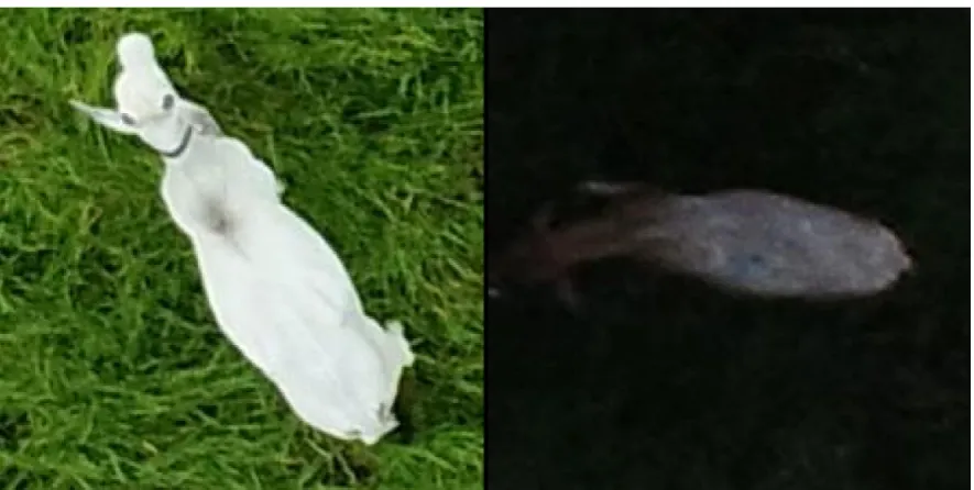
Figure 1.Examples of well-lit (left) and too dark conditions (right).
2. Materials and Methods
80
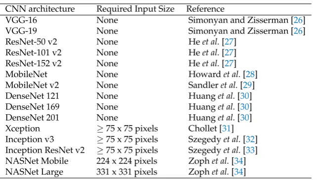
2.1. Image Dataset
81
The UAV used in the experiments was a DJI Phantom 4 Pro, equipped with an 20-MPixel camera.
82
The 4:3 aspect ratio was adopted in the experiments, resulting in images with 4864 x 3648 pixels.
83
Missions were carried out at the Canchim farm, São Carlos, Brazil (21◦58’28” S, 47◦50’59” W) at 11
84
dates over the year of 2018. Camera settings were all kept on automatic, except exposition, which used
85
the presets “sunny” and “overcast” depending on weather conditions. Images were captured from an
86
altitude of 30 m with respect to the take-off position. This altitude provided a fine GSD (approximately
87
1 cm/pixel) without disturbing the animals, which showed no reaction when the aircraft flew over
88
them. Altitude and GSD had variations of up to 20% due to the ruggedness of the terrain. Frontal
89
and side image overlap images were both set to 70%. Each animal is represented by 13,000 pixels in
90
average – this number varies considerably with the size and position of the animals, as well as with
91
the actual altitude at the moment of capture. The images cover a wide range of capture conditions, and
92
animals from both Canchim and Nelore breeds were present during all flights. Illumination varied
93
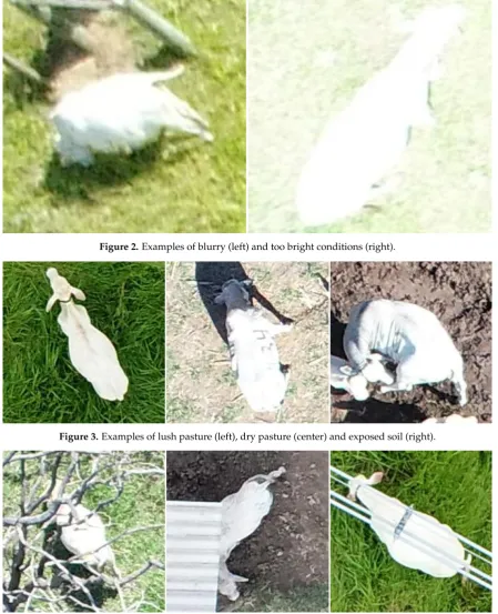
from well-lit to very dark conditions (Figure 1), which is due not only to the weather, but also to
94
condition variations in the same flight. The contrast between animals and background also varied
95
significantly – low contrast situations were caused by both movement blur and excessive brightness
96
(Figure 2). Because images were captured at different times of the year, soil conditions also varied
97
(Figure 3). Different degrees of animal occlusions are also present (Figure 4). A total of 19,097 images
98
were captured, from which 1,853 images containing at least part of an animal were selected for the
99
experiments. The maximum number of animals in a single image was 15.
100
Two datasets were generated from the original images. In the first one, 224 x 224 pixel squares
101
were associated to all animals in all images, carefully encompassing each individual. Animals at the
102
edges of the images were only considered if at least 50% of their bodies were visible. While the targeted
103
animal was always centered, there were cases in which image blocks included parts of other animals
104
due to close proximity. A total of 8,629 squares containing animals were selected; the same number
105
of squares was randomly selected to represent the background. This dataset was generated with the
106
objective of determining the best possible accuracy that can be achieved when all objects of interest are
107
perfectly framed by the image blocks to be classified. In the second dataset, images were subdivided
108
into image blocks using a regular grid with 224-pixel spacing both horizontally and vertically. This
Figure 2.Examples of blurry (left) and too bright conditions (right).
Figure 3.Examples of lush pasture (left), dry pasture (center) and exposed soil (right).
Figure 4.Examples of animal oclusions: tree branches (left), shed roof (middle), electrical wires (right).
value was chosen because 224 x 224 pixels is the default input size for many of the CNNs tested in
110
this work and, additionally, blocks of this size encompass almost perfectly most of the animals present
111
in the images. Blocks were then labelled as “cattle” and “non-cattle”; to be labelled as “cattle”, a
112
block should contain at least a few pixels that could be undoubtedly associated to an animal without
113
having any other block (or the entire image) as reference. This criterion is subjective and susceptible to
114
inter- and intra-rater inconsistencies [24], but this was the most viable approach given the amount and
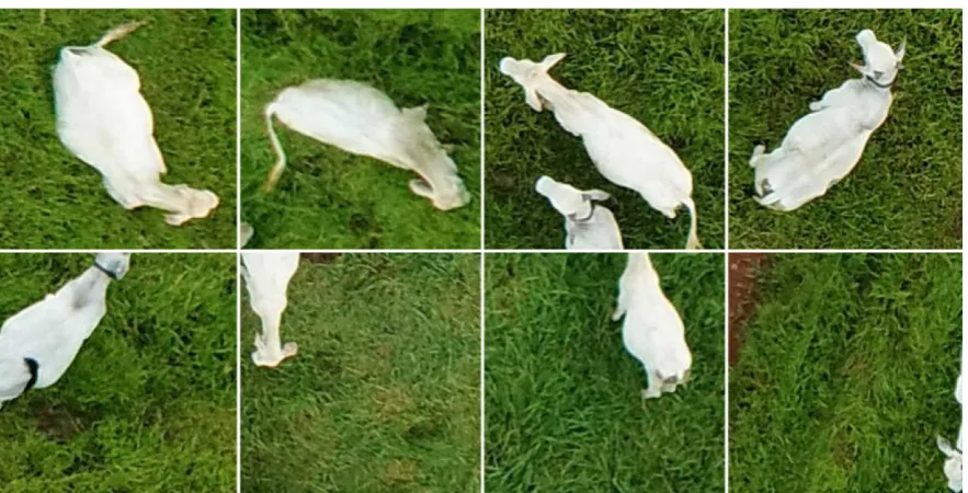
Figure 5.Examples of image blocks containing carefully framed animals (upper row) and image blocks generated using a regular grid (bottom row).
Figure 6.Workflow used to train all models considered in the experiments.
characteristics of the images. A total of 14,489 image blocks were labelled as “cattle”; the number of
116
“non-cattle” blocks was much higher but, in order to avoid problems associated with class imbalance,
117
only 14,489 randomly selected “non-cattle” blocks were used in the experiments. Both image datasets
118
were manually annotated by the same person. Some examples of “cattle” image blocks present in each
119
dataset are shown in Figure 5.
120
2.2. Experimental Setup
121
Figure 6 shows the basic workflow used to train each of the models tested in this study.
122
First, the original dataset containing all labelled image blocks was divided into a training
123
(80% of the samples) and a test dataset (20%). A validation set was not used because the model
124
hyperparameters were defined having previous experiments as reference, as described later in this
125
section. As a result, the training and test datasets always contained, respectively, 13,806 and 3,452
126
samples when the first dataset was adopted (careful animal framing), and 23,182 and 5,796 samples
127
when the second dataset was used (regular grid). In order to avoid biased results due to skewed data
128
distributions caused by the random dataset division, a 10-fold cross-validation was adopted. In other
129
words, 10 models were trained for each pair of input dimension and CNN considered.
130
As mentioned before, all image blocks generated during the labelling process had 224 x 224 pixels.
131
In order to simulate coarser GSDs, the original image blocks were downsampled to 112 x 112 pixels
132
and 56 x 56 pixels, simulating GSDs of 2 and 4 cm/pixel or, equivalently, simulating flight altitudes
133
of 60 and 120 m, which is the current legal limit in most countries without the need for some special
134
exemption [1].
135
The experiments were carried out using the Keras library (keras.io, version 2.2.4) with TensorFlow
136
v. 1.4. Keras library had available all models used in the experiments, thus avoiding the need for direct
137
coding orusing third-party sources. With this setup, most CNNs could be trained using images of any
138
dimension as input, even when using pretrained networks (transfer learning), as was the case in this
139
study. However, there are some architectures that require the input dimensions to be either a fixed or
Table 1.CNN architectures tested in the experiments.
CNN architecture Required Input Size Reference
VGG-16 None Simonyan and Zisserman [26]
VGG-19 None Simonyan and Zisserman [26]
ResNet-50 v2 None Heet al.[27]
ResNet-101 v2 None Heet al.[27]
ResNet-152 v2 None Heet al.[27]
MobileNet None Howardet al.[28]
MobileNet v2 None Sandleret al.[29]
DenseNet 121 None Huanget al.[30]
DenseNet 169 None Huanget al.[30]
DenseNet 201 None Huanget al.[30]
Xception ≥75 x 75 pixels Chollet [31]
Inception v3 ≥75 x 75 pixels Szegedyet al.[32]
Inception ResNet v2 ≥75 x 75 pixels Szegedyet al.[33]
NASNet Mobile 224 x 224 pixels Zophet al.[34]
NASNet Large 331 x 331 pixels Zophet al.[34]
above a certain lower limit (see Table 1). In cases like these, it is necessary to upsample the images
141
after downsampling to meet the requirements of those architectures. It is important to emphasize that
142
a direct comparison between architectures is still possible even if the input dimensions are different,
143
because the downsampling causes a loss of information that is not reverted by the upsampling.
144
Fifteen different CNN architectures were tested (Table 1) using the following hyperparameters:
145
fixed learning rate of 0.0001, 10 epochs (most models converged with fewer than 5 epochs), mini-batch
146
size of 128 (larger values caused memory problems with deeper architectures) and sigmoid activation
147
function. Transfer learning was applied by using models pretrained on the Imagenet dataset [25]
148
and freezing all convolutional layers and updating only the top layers. Training was performed in a
149
workstation equipped with two RTX-2080 Ti GPUs.
150
Finally, model assessment was carried out by taking the trained models and applying them to the independent test sets. Four performance metrics were extracted:
Accuracy= (TP+TN)/(TP+TN+FP+FN), (1)
Precision=TP/(TP+FP), (2)
Recall =TP/(TP+FN), (3)
F1Score=2∗(Recall∗Precision)/(Recall+Precision), (4) where TP, TN, FP and FN are the number of true positives, true negatives, false positives and false
151
negatives, respectively.
152
3. Results
153
Table 2 summarizes the results obtained having the first dataset as reference (“cattle” image blocks
154
centered exactly at the position of each animal). The objective of this experiment was to assess the
155
performance of the models when trained with samples carefully generated to represent each class
156
as consistently as possible. Only the 224 x 224 pixel samples were used in this case because this
157
experiment was carried out only to serve as a reference for the more realistic one shown in Table 3.
158
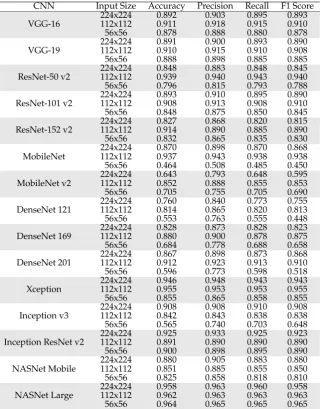
Table 3 is similar to Table 2, except the samples used in the training were generated using the
159
second dataset (regular grid). This is a more challenging situation, as some “cattle” image blocks may
160
contain only small parts of the animals which need to be properly detected by the models. In addition,
161
Figure 7 shows graphically the average and range of accuracies obtained for each model.
162
Table 4 shows the average time that it took to train each CNN over one epoch.
Table 2.Results obtained using the dataset labelled with exact animal locations.
CNN Accuracy Precision Recall F1 Score
VGG-16 0.972 0.973 0.973 0.970
VGG-19 0.973 0.973 0.973 0.975
ResNet-50 v2 0.977 0.978 0.978 0.975
ResNet-101 v2 0.983 0.985 0.985 0.985
ResNet-152 v2 0.967 0.970 0.970 0.965
MobileNet 0.983 0.980 0.980 0.983
MobileNet v2 0.787 0.855 0.790 0.778
DenseNet 121 0.852 0.895 0.868 0.865
DenseNet 169 0.935 0.943 0.933 0.935
DenseNet 201 0.935 0.945 0.938 0.938
Xception 0.969 0.968 0.968 0.968
Inception v3 0.979 0.975 0.975 0.975
Inception ResNet v2 0.983 0.983 0.983 0.985
NASNet Mobile 0.857 0.890 0.858 0.853
NASNet Large 0.992 0.993 0.993 0.995
Table 3.Results obtained using the dataset labelled with exact animal locations.
CNN Input Size Accuracy Precision Recall F1 Score
224x224 0.892 0.903 0.895 0.893
VGG-16 112x112 0.911 0.918 0.915 0.910
56x56 0.878 0.888 0.880 0.878
224x224 0.891 0.900 0.893 0.890
VGG-19 112x112 0.910 0.915 0.910 0.908
56x56 0.888 0.898 0.885 0.885
224x224 0.848 0.883 0.848 0.845
ResNet-50 v2 112x112 0.939 0.940 0.943 0.940
56x56 0.796 0.815 0.793 0.788
224x224 0.893 0.910 0.895 0.890
ResNet-101 v2 112x112 0.908 0.913 0.908 0.910
56x56 0.848 0.875 0.850 0.845
224x224 0.827 0.868 0.820 0.815
ResNet-152 v2 112x112 0.914 0.890 0.885 0.890
56x56 0.832 0.865 0.835 0.830
224x224 0.870 0.898 0.870 0.868
MobileNet 112x112 0.937 0.943 0.938 0.938
56x56 0.464 0.508 0.485 0.450
224x224 0.643 0.793 0.648 0.595
MobileNet v2 112x112 0.852 0.888 0.855 0.853
56x56 0.705 0.755 0.705 0.690
224x224 0.760 0.840 0.773 0.755
DenseNet 121 112x112 0.814 0.865 0.820 0.813
56x56 0.553 0.763 0.555 0.448
224x224 0.828 0.873 0.828 0.823
DenseNet 169 112x112 0.880 0.900 0.878 0.875
56x56 0.684 0.778 0.688 0.658
224x224 0.867 0.898 0.873 0.868
DenseNet 201 112x112 0.912 0.923 0.913 0.910
56x56 0.596 0.773 0.598 0.518
224x224 0.946 0.948 0.943 0.943
Xception 112x112 0.955 0.953 0.953 0.955
56x56 0.855 0.865 0.858 0.855
224x224 0.908 0.908 0.910 0.908
Inception v3 112x112 0.842 0.843 0.838 0.838
56x56 0.565 0.740 0.703 0.648
224x224 0.925 0.933 0.925 0.923
Inception ResNet v2 112x112 0.891 0.890 0.890 0.890
56x56 0.900 0.898 0.895 0.890
224x224 0.880 0.905 0.883 0.880
NASNet Mobile 112x112 0.851 0.885 0.855 0.850
56x56 0.825 0.858 0.818 0.810
224x224 0.958 0.963 0.960 0.958
NASNet Large 112x112 0.962 0.963 0.963 0.963
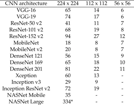
Table 4.Average training time for different input sizes (in seconds per epoch).
CNN architecture 224 x 224 112 x 112 56 x 56
VGG-16 65 14 6
VGG-19 74 17 6
ResNet-50 v2 41 11 7
ResNet-101 v2 68 19 8
ResNet-152 v2 94 27 12
MobileNet 18 8 7
MobileNet v2 20 8 7
DenseNet 121 56 15 9
DenseNet 169 65 18 10
DenseNet 201 81 22 11
Xception 60 13
-Inception v3 29 9
-Inception ResNet v2 72 19
-NASNet Mobile 35 -
-NASNet Large 334* -
Figure
7.
Range
of
accuracies
obtained
for
each
CNN
ar
chitectur
e.
The
thr
ee
bars
associated
to
each
ar
chitectur
e
corr
espond
to
input
sizes
of
224x224
(left),
112x112
(middle)
and
56x56
(right).
The
cir
cle
in
each
bar
repr
esents
the
average
accuracy
,
and
the
bottom
and
top
extr
emities
repr
esent
the
lowest
and
highest
accuracies
observed
during
the
application
of
the
10-fold
cr
4. Discussion
164
The results shown in Table 2 reveal that most models were able to reach accuracies above 95%
165
when training and test image blocks were carefully generated to provide the best characterization of
166
each class. Very deep structures, like NasNet Large, were able to yield accuracies close to 100%. In
167
practice, using models trained this way is challenging: the positions of the animals in a new image to
168
be analyzed by the model will not be known a priori (otherwise the problem would be solved already),
169
so image blocks cannot be properly generated to perfectly encompass the animals to be detected. One
170
possible solution to this problem is to sweep the entire image using a sliding window in such a way
171
each animal will appear, at least partially, in multiple image blocks to be analyzed by the model. This
172
approach, which has been explored by [15,17,18], enables the construction of a heat map showing the
173
likely positions of the animals in the image. The problem with this approach is that the number of
174
image blocks to be analyzed may be very high; on the other hand, applying the models is much faster
175
than training them, which makes this approach adequate in many situations.
176
Overall, CNNs were remarkably robust to almost all variations in illumination conditions.
177
No noticeable differences in accuracy were observed when only images with illumination issues
178
(insufficient and excessive brightness, shadows) were considered. The only exception was with
179
the presence of severe specular reflection, in which case the contrast between animals and ground
180
tended to become too slight for the models to detect then correctly. Excessively blurred images also
181
caused problems. Specular reflection and blur explain most of the errors observed when the dataset
182
labelled with exact animal locations was used. Models like NasNet Large and the ResNet were fairly
183
robust even under these poor conditions. Those models did not reach 100% accuracy because, in a
184
few instances, the number of problematic images in the test set was proportionally much higher, a
185
consequence of the randomness of the division process.
186
As expected, accuracies were lower when the regular grid was used. Interestingly, for 12 of the 15
187
models, the best results were achieved using the 112x112 input size. This indicates that the ideal GSD
188
for cattle detection is 2 cm/pixel. At a first glance, this may seem counterintuitive, because higher
189
resolutions tend to offer more information to be explored by the models. However, the way most CNNs
190
architectures are designed (filter and convolution sizes), features related to cattle can be more effectively
191
extracted at this GSD. As an added bonus, these results indicate that we could fly twice as high (thus
192
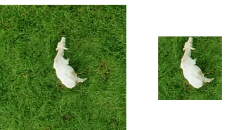
covering a much larger area) without losing any accuracy. It is worth mentioning that another method
193
for simulating different GSDs was considered, in which the entire image is downsampled and then the
194
regular grid is applied, instead of first applying the grid and then downsampling the image blocks.
195
The main difference between both approaches is that in the latter the relative area occupied by animals
196
within each block is kept the same, while in the former the area occupied by the animals will decrease
197
in the same proportion as the downsampling. In both cases, the number of pixels associated to the
198
animals will be exactly the same, but in the approach adopted here the amount of background will be
199
much lower (Figure 8). Some limited experiments were performed using the alternative approach, and
200
a drop in accuracy was observed for all models but Inception v3, for which the accuracy was slightly
201
better.
202
The drop in accuracy observed when the regular grid approach was adopted is almost exclusively
203
due to many image blocks annotated as “cattle” having very few pixels actually associated to an
204
animal (Figure 8). Because such blocks contain mostly background, it may be difficult for the model
205
to learn the correct features associated to cattle during training – if the wrong features are learnt, the
206
potential for misclassifications rise considerably. The reverse problem occurs during the application
207
of the model: since background is so dominant, the amount of pixels associated to animals may not
208
be enough for proper detection. However, considering the amount of “cattle” blocks showing only a
209
small fraction of the animals’ bodies, it is remarkable that some models were able to yield accuracies
210
above 95%. It is also important to remark that errors of this kind are not very damaging: blocks with
211
small animal parts will almost certainly have one or more neighboring blocks containing the remainder
212
of the animal, in which case correct detection is more likely. Errors caused by missed small parts can
Figure 8. Examples of the two possible approaches to simulate coarser GSDs. In the left, the entire image is downsampled and then the regular grid is applied; in the right, the grid is first applied and then image blocks are downsampled.
Figure 9.Examples of “cattle” blocks with very small animal parts visible (red elipses).
be compensated by other image processing techniques, which can be used to refine the delineation
214
of the animals. There are some approaches that tackle this problem explicitly, like region proposal
215
networks [4] and the concept of anchor boxes used in YOLO [7]. These alternative techniques will be
216
investigated in future experiments.
217
Most CNN architectures performed well under the experimental conditions of this study. Taking
218
only accuracy into consideration, the most successful CNN was NasNet Large. The very deep and
219
complex structure associated to this architecture made it very robust to all the challenging conditions
220
found in the dataset used in the experiments. The Xception architecture had slightly lower accuracies,
221
especially when the 112x112 input size was used, but its training time was several times faster than
222
that associated to NasNet Large. Among the lightest architectures (mostly developed for use in mobile
223
devices), MobileNet (version 1) showed the best performance. All trained models took less than 1
224
second to fully analyse a 4864 x 3648-pixel image when ran in the workstation mentioned in Section
225
2.2. Operational time differences between models are expected to increase when devices with less
226
computational power are used (e.g. mobile devices), but testing the models under more restricted
227
setups was beyond the scope of this study.
As mentioned before, most of the experiments were performed with animals of the Canchim
229
breed, whose colors range from white to light beige, with some darker coating occurring in some
230
animals. Because of its Nelore roots, it shares many visual characteristics with this breed, and as a
231
result the models generated in this work were also effective detecting Nelore animals. Other breeds
232
would probably require the training of new models, and the degree of success that can be potentially
233
achieved in each case would have to be investigated. However, taking into consideration the results
234
reported in the literature for other breeds and other experimental setups, it seems evident that deep
235
learning architectures are remarkably successful in extracting relevant information that can lead to
236
accurate detection of cattle in images captured by UAVs.
237
5. Conclusion
238
This article presented a study on the use of deep learning models for the detection of cattle
239
(Canchim breed) in UAV images. The experiments were designed to test the robustness of 15 different
240
CNN architectures to factors like low illumination, excessive brightness, presence of blur, only small
241
parts of the animal body visible, among others. Most models showed a remarkable robustness to such
242
factors, and if a few precautions are taken during the imaging missions, accuracy rates can be close to
243
100%. In terms of accuracy, NasNet Large yielded the best results, with the Xception architecture also
244
producing very high accuracies with a faction of NasNet’s training times. The most accurate results
245
were obtained with a GSD of 2cm/pixel, indicating that images can be captured at relatively high
246
flight altitudes without degrading the results. Future work will focus on testing new approaches for
247
animal detection. In particular, future experiments will investigate how techniques that generate a
248
bounding box around the objects of interest (e.g. YOLO) and semantic segmentation methods perform
249
under the same conditions tested in this work. At the same time, the image dataset will continue to
250
receive new images, thus expanding even more the variety of conditions. Breeds other than Canchim
251
are also expected to be included. The image database used in this experiment is currently unavailable
252
for external researchers, but this will likely change as soon as the database is properly organized and
253
some restrictions are lifted.
254
6. Acknowledgements
255
This work was funded by Fapesp under grant number 2018/12845-9, and Embrapa under grant
256
number 22.16.05.021.00.00. The authors would also like to thank Nvidia for donating the Titan XP
257
GPU used in part of the experiments.
258
259
1. Barbedo, J.G.A.; Koenigkan, L.V. Perspectives on the use of unmanned aerial systems to monitor cattle.
260
Outlook on Agriculture2018,47, 214–222. doi:10.1177/0030727018781876.
261
2. Barbedo, J.G.A. A Review on the Use of Unmanned Aerial Vehicles and Imaging Sensors for Monitoring
262
and Assessing Plant Stresses.Drones2019,3. doi:10.3390/drones3020040.
263
3. Redmon, J.; Farhadi, A. YOLOv3: An Incremental Improvement. ArXiv2018,abs/1804.02767.
264
4. Ren, S.; He, K.; Girshick, R.; Sun, J. Faster R-CNN: Towards Real-Time Object Detection with Region
265
Proposal Networks. IEEE Transactions on Pattern Analysis and Machine Intelligence2017,39, 1137–1149.
266
doi:10.1109/TPAMI.2016.2577031.
267
5. Chen, L.C.; Papandreou, G.; Schroff, F.; Adam, H. Rethinking Atrous Convolution for Semantic Image
268
Segmentation. ArXiv2017,abs/1706.05587.
269
6. Ronneberger, O.; Fischer, P.; Brox, T. U-Net: Convolutional Networks for Biomedical Image Segmentation.
270
ArXiv2015,abs/1505.04597.
271
7. Redmon, J.; Farhadi, A. YOLO9000: Better, Faster, Stronge.ArXiv2016,abs/1612.08242.
272
8. Kellenberger, B.; Marcos, D.; Tuia, D. Detecting mammals in UAV images: Best practices to address a
273
substantially imbalanced dataset with deep learning. Remote Sensing of Environment2018,216, 139 – 153.
274
doi:https://doi.org/10.1016/j.rse.2018.06.028.
9. Chrétien, L.P.; Théau, J.; Ménard, P. Visible and thermal infrared remote sensing for the detection of
276
white-tailed deer using an unmanned aerial system. Tools and Technology2016,40, 181–191.
277
10. Franke, U.; Goll, B.; Hohmann, U.; Heurich, M. Aerial ungulate surveys with a combination of infrared
278
and high-resolution natural colour images. Animal Biodiversity and Conservation2012,35, 285–293.
279
11. Witczuk, J.; Pagacz, S.; Zmarz, A.; Cypel, M. Exploring the feasibility of unmanned aerial vehicles and
280
thermal imaging for ungulate surveys in forests - preliminary results.International Journal of Remote Sensing
281
2017,doi: 10.1080/01431161.2017.1390621.
282
12. Lhoest, S.; Linchant, J.; Quevauvillers, S.; Vermeulen, C.; Lejeune, P. How many hippos (HOMHIP):
283
algorithm for automatic counts of animals with infra-red thermal imagery from UAV.International Archives
284
of the Photogrammetry, Remote Sensing and Spatial Information Sciences2015, pp. 355–362.
285
13. Mulero-Pázmány, M.; Stolper, R.; Essen, L.; Negro, J.J.; Sassen, T. Remotely Piloted Aircraft Systems as a
286
Rhinoceros Anti-Poaching Tool in Africa.PLoS ONE2014,9, e83873.
287
14. Vermeulen, C.; Lejeune, P.; Lisein, J.; Sawadogo, P.; Bouche, P. Unmanned Aerial Survey of Elephants.
288
PLoS ONE2013,8, e54700.
289
15. Chamoso, P.; Raveane, W.; Parra, V.; González, A. UAVs Applied to the Counting and Monitoring of
290
Animals. Advances in Intelligent Systems and Computing.Advances in Intelligent Systems and Computing
291
2014,291, 71–80.
292
16. Longmore, S.; Collins, R.; Pfeifer, S.; Fox, S.; Mulero-Pázmány, M.; Bezombes, F.; Goodwin, A.; Juan Ovelar,
293
M.; Knapen, J.; Wich, S. Adapting astronomical source detection software to help detect animals in thermal
294
images obtained by unmanned aerial systems.International Journal of Remote Sensing2017,38, 2623–2638.
295
17. Rivas, A.; Chamoso, P.; González-Briones, A.; Corchado, J. Detection of Cattle Using Drones and
296
Convolutional Neural Networks.Sensors2018,18, 2048.
297
18. Rahnemoonfar, M.; Dobbs, D.; Yari, M.; Starek, M. DisCountNet: Discriminating and Counting Network
298
for Real-Time Counting and Localization of Sparse Objects in High-Resolution UAV Imagery. Remote
299
Sensing2019,11, 1128.
300
19. Shao, W.; Kawakami, R.; Yoshihashi, R.; You, S.; Kawase, H.; Naemura, T. Cattle detection and counting
301
in UAV images based on convolutional neural networks. International Journal of Remote Sensing2020,
302
41, 31–52.
303
20. Jung, S.; Ariyur, K.B. Strategic Cattle Roundup using Multiple Quadrotor UAVs. International Journal of
304
Aeronautical and Space Sciences2017,18, 315–326.
305
21. Nyamuryekung’e, S.; Cibils, A.; Estell, R.; Gonzalez, A. Use of an Unmanned Aerial Vehicle – Mounted
306
Video Camera to Assess Feeding Behavior of Raramuri Criollo Cows.Rangeland Ecology & Management
307
2016,69, 386–389.
308
22. Andrew, W.; Greatwood, C.; Burghardt, T. Aerial Animal Biometrics: Individual Friesian Cattle
309
Recovery and Visual Identification via an Autonomous UAV with Onboard Deep Inference. ArXiv
310
2019,abs/1907.05310v1.
311
23. Webb, P.; Mehlhorn, S.A.; Smartt, P. Developing Protocols for Using a UAV to Monitor Herd Health.
312
ASABE Annual International Meeting2017, p. 1700865.
313
24. Bock, C.; Poole, G.; Parker, P.; Gottwald, T. Plant disease severity estimated visually, by digital photography
314
and image analysis, and by hyperspectral imaging.Critical Reviews in Plant Sciences2010,29, 59–107.
315
25. Deng, J.; Dong, W.; Socher, R.; Li, L.J.; Li, K.; Fei-Fei, L. ImageNet: A Large-Scale Hierarchical Image
316
Database. CVPR09, 2009.
317
26. Simonyan, K.; Zisserman, A. Very Deep Convolutional Networks for Large-Scale Image Recognition.
318
ArXiv2014,abs/1409.1556v6.
319
27. He, K.; Zhang, X.; Ren, S.; Sun, J. Deep Residual Learning for Image Recognition. ArXiv2015,
320
abs/1512.03385.
321
28. Howard, A.; Zhu, M.; Chen, B.; Kalenichenko, D.; Wang, W.; Weyand, T.; Andreetto, M.; Adam, H.
322
MobileNets: Efficient Convolutional Neural Networks for Mobile Vision Applications. ArXiv2017,
323
abs/1704.04861.
324
29. Sandler, M.; Howard, A.; Zhu, M.; Zhmoginov, A.; Chen, L.C. MobileNetV2: Inverted Residuals and Linear
325
Bottlenecks. ArXiv2019,abs/1801.04381v4.
326
30. Huang, G.; Liu, Z.; Maaten, L.; Weinberger, K. Densely Connected Convolutional Networks. ArXiv2018,
327
abs/1608.06993v5.
31. Chollet, F. Xception: Deep Learning with Depthwise Separable Convolutions.ArXiv2017,abs/1610.02357v3.
329
32. Szegedy, C.; Vanhoucke, V.; Ioffe, S.; Shlens, J.; Wojna, Z. Rethinking the Inception Architecture for
330
Computer Vision. ArXiv2015,abs/1512.00567.
331
33. Szegedy, C.; Ioffe, S.; Vanhoucke, V.; Alemi, A. Inception-v4, Inception-ResNet and the Impact of Residual
332
Connections on Learning. ArXiv2016,abs/1602.07261v2.
333
34. Zoph, B.; Vasudevan, V.; Shlens, J.; Le, Q. Learning Transferable Architectures for Scalable Image
334
Recognition.ArXiv2018,abs/1707.07012v4.