Identifying Potentially Flawed Items in the Context of Small Sample IRT Analysis
Panagiotis Fotaris, Theodoros Mastoras, Ioannis Mavridis, and Athanasios Manitsaris
Department of Applied Informatics University of Macedonia
Thessaloniki, Greece
{paf, mastoras, mavridis, manits}@uom.gr
Abstract—Although Classical Test Theory has been used by the
measurement community for almost a century, Item Response Theory has become commonplace for educational assessment development, evaluation and refinement in recent decades. Its potential for improving test items as well as eliminating the ambiguous or misleading ones is substantial. However, in order to estimate its parameters and produce reliable results, IRT requires a large sample size of examinees, thus limiting its use to large-scale testing programs. Nevertheless, the accuracy of parameter estimates becomes of lesser importance when trying to detect items whose parameters exceed a threshold value. Under this consideration, the present study investigates the application of IRT-based assessment evaluation to small sample sizes through a series of simulations. Additionally, it introduces a set of quality indices, which exhibit the success rate of identifying potentially flawed items in a way that test developers without a significant statistical background can easily comprehend and utilize.
Keywords - item response theory, computer aided assessment,
item quality, educational measurement, learning assessment evaluation, e-learning, psychometrics.
I. INTRODUCTION
Following the recent advances in Information and Communications Technology (ICT) as well as the growing popularity of distance learning, an ever-increasing number of academic institutions worldwide have embraced the idea that the educational process can be greatly enhanced through the use of Computer Aided Assessment (CAA) tools [1][2][3][4]. Some of the benefits of these tools include the potential for generating rapid individualized feedback [5][6], the reduction of the marking load on staff [7], the ability to include multimedia elements in test items [8], the availability of administrative and statistical data [9], and, most importantly, the assessment of the examinees’ knowledge [10].
Self-assessment tests, while commonly portrayed as the most popular technique to enhance learning [11] and evaluate the learning status of each examinee [12], have been criticized extensively on account of their perceived lack of reliability. Moreover, both research and experience show that a substantial number of test items (questions) are flawed at the initial stage of their development. As a result, test developers can expect nearly 50% of their items to fail to perform as intended, thus leading to unreliable results with respect to examinee performance [13]. It is, therefore, of the utmost importance to ensure that the individual test items are of the highest possible quality, since an inferior
item could have an inordinately large effect on scores and consequently pose a serious threat to overall test effectiveness.
Among the dominant methodological theories in item evaluation using item response data are Classical Test Theory (CTT) [14] and Item Response Theory (IRT) [15]. The former is essentially a loose collection of techniques for analyzing test functionality, including but not limited to indices of score reliability, item difficulty, item discrimination, and the distribution of examinee responses across the available range of responses [16]. Many of these techniques were generated in the 19th and 20th centuries by Pearson, Spearman, Thurstone, and others [17]. CTT is built around the idea that the observed score an examinee attains on a test is a function of that examinee’s “true score” and error. Although its relatively weak theoretical assumptions make CTT easy to apply in many testing situations [18], this approach has a number of well-documented shortcomings. These include (a) the use of item indices whose values depend on the particular group of examinees with which they are obtained, and (b) examinee ability estimates that depend on the particular choice of items selected for a test [19]. Additionally, CTT is not as likely to be as sensitive to items that discriminate differentially across different levels of ability (or achievement), it does not work as well when different examinees take different sets of items, and it is not as effective in identifying items that are statistically biased [20][21].
On the other hand, IRT is more theory-grounded and models the probabilistic distribution of the examinees’ success at item level. As its name indicates, IRT primarily focuses on the item-level information in contrast to the CTT’s primary focus on test-level information [22]. Based on nonlinear models that plot the measured latent variable and the item response, it enables independent estimation of item and person parameters and local estimation of measurement error [23]. The IRT framework encompasses a group of models, with the applicability of each model in a particular situation depending on the nature of the test items and the viability of different theoretical assumptions about them. Models that use a single ability to describe quantitative differences among examinees and among items are referred to as unidimensional (UIRT), whereas those for multiple abilities are called multidimensional (MUIRT).
parameters for each item, α, b and c respectively. The α parameter, also known as item slope, is analogous to CTT’s item-test biserial correlation and measures the discriminating power of the item, while the b parameter is an index of item difficulty; consequently, the latter increases in value as items become more difficult. In contrast to the p -value used in CTT, b is theoretically not dependent on the ability level of the sample of examinees tested. Finally, the c
parameter, commonly called the guessing or the pseudo-guessing parameter, is defined as the probability of a very low-ability test-taker answering the item correctly [26]. All three parameters are present in the following equation called Item Response Function (IRF) that defines the three-parameter logistic model (3PL) for dichotomous data. IRF gives the probability of a correct response to item i by an examinee with ability θ. When displayed graphically, it is called the Item Response Curve (IRC).
1
1 | , 1, 2, ..., .
1 i i
i
i i i i Da b
c
P P X c i n
e
In Equation (1), Xi is the score for item i, with Xi = 1 for
a correct response and Xi = 0 for an incorrect response. θ is
the numerical value of the trait that reflects the examinee’s level of ability, achievement, skill, or other major characteristic, which is measured by the test. αi, bi, and ci
are item parameters, and D is a scaling constant. In the two-parameter logistic model (2PL) the c parameter is fixed at a specific value rather than estimated, with both the α and c
parameters fixed at specific values in the one-parameter logistic model (1PL).
Theoretically, IRT overcomes the circular dependency of CTT’s item / person parameters and its models produce item statistics independent of examinee samples, and person statistics independent of the particular set of items administered [27]. This invariance property of IRT’s item and person statistics has been widely accepted within the measurement community, resulting in the widespread application of IRT models to large-scale educational testing programs.
However, the aforementioned models have not proven popular outside these programs due to the complex nature of the item parameter estimation associated with them. To ensure that all IRT parameters are correctly estimated, every single item needs to be tested on a large number of examinees so as to define its properties [28]. Unless this condition is fulfilled, the benefits of using IRT might not be attained, i.e., the success of IRT applications requires a satisfactory fit between the model and the data. It is generally accepted that a minimum sample size of 20 items and 200 examinees is sufficient to fit the one parameter logistic model [29][30], while much larger sample sizes (e.g., 60 items and 1,000 examinees) are needed for the three parameter logistic IRT model [31].
Although a number of researchers have proposed smaller sample sizes than those specified above [32][33], it remains difficult for educators who teach small- or medium-sized classes to find a satisfying number of test-takers. So far,
little research has been done to investigate whether the potential advantages of an IRT model can still be achieved in such an environment. Fotaris et al. [34] introduced a methodological and architectural framework for extending an LMS with IRT–based assessment test calibration. By defining a set of validity rules, test developers are able to set the acceptable limits for all IRT parameters before administering the test. The enhanced LMS subsequently applies these rules to the parameters produced by the IRT analysis in order to detect potentially flawed items and report them for reviewing. Since this system has only been used on a pilot basis, the present study is focused on exploring the benefits, limitations and accuracy of incorporating IRT analysis given limited sample sizes before its adoption in actual academic courses.
The next sections of this paper will introduce two types of quality indices and describe the simulation study design and process. The results of the study will be presented in the final section, together with a discussion about the impact of the examinees’ ability distribution on the performance of the IRT analysis.
II. ASSESSMENT QUALITY INDICES
As previously mentioned, it is necessary to estimate parameters α, b, and c for each test item when using a three-parameter logistic model. This procedure, also called item calibration, is typically performed by software that employs joint maximum likelihood (JML), conditional maximum likelihood (CML), or marginal maximum likelihood (MML) methods [35]. Although its level of accuracy affects the success rate of potentially flawed items detection, the latter is not directly obtained from the item fit indices used in the various goodness-of-fit studies [36][37][38][39]. Therefore, the present paper introduces new indices to describe this exact success rate in a way that test developers without a profound statistical background will be able to fully comprehend and utilize.
Let τi denote the true value of one IRT parameter (α, b,
or c) for item i, and ˆτi its corresponding estimate. Accordingly, let A{τi} denote the set of the assessment test’s
true parameter values, with (A, ≤) being totally ordered, and
ˆ ˆτi
A the set of its corresponding estimates, with (Â, ≤)
being totally ordered, as well. Sets N and Nˆ contain the
indices i of the elements in A and  respectively.
: τi
,
1,2,...,
N i A i n , (2)
ˆ
ˆ : τˆ , 1, 2,...,
i
N i A i n , (3)
Thus, given a test with n dichotomous items, all of the aforementioned sets have the same cardinality n:
ˆ ˆ
Sets N( )q and Nˆ( )q contain the indices i of items whose parameter values are equal to or lower than a threshold value q; they can be described as follows:
( )q : τi , τi , 1,2,...,
N i A q i n , (5)
( ) ˆ
ˆ : τˆ , τˆ , 1, 2,...,
q i i
N i A q i n , (6)
with N( )q referring to the true parameter values and Nˆ( )q
to the estimates, respectively. In a similar manner, the sets containing the indices i of items whose parameter values are equal to or greater than a threshold value q, can be described thus:
( )q : τi , τi , 1,2,...,
N i A q i n , (7)
( ) ˆ
ˆ : τˆ , τˆ , 1, 2,...,
q i i
N i A q i n , (8)
with N( )q referring to the true parameter values, and Nˆ( )q
to the estimates, respectively. Let NL r % be a subset of N
with its cardinality being a percentage (r%) of the cardinality of A. NL r % contains the indices i of items whose parameter values belong to the lower set of
A,
(9). Likewise, let NˆL r % be a subset of Nˆ with its cardinality being a percentage (r%) of the cardinality of Aˆ. % ˆ
L r
N contains the indices i of items whose parameter
values belong to the lower set of
Aˆ, (10).
% % % ( %) : τ , τ , τ , τ τ τ ,% , , 1, 2,.. ,.
i j
L r
i j L r j i L r
L r
N i A A
i N j N
N A r i j n
(9)
% % % % ˆ ˆ ˆ : τˆ , τˆ , ˆ ˆ ˆ ˆ ˆ ˆ τ , τ τ τ , ˆ ˆ% , , 1, 2,...,
i j
L r
i j L r j i L r
L r
N i A A
i N
j n
j N
N A r i
(10)The same logic is used to denote the sets NU r % and
% ˆ
U r
N , with the only difference being that they contain the
indices i of items whose parameter values belong to the
upper set of
A,
and
Aˆ, , respectively.
% % % ( %) : τ , τ , τ , τ τ τ ,% , , 1, 2,...,
i j
U r
i j U r j i U r
U r
N i A A
i N j N
N A r i j n
(11)
% % % % ˆ ˆ ˆ : τˆ , τˆ , ˆ ˆ ˆ ˆ ˆ ˆ τ , τ τ τ , ˆ ˆ% , , 1, 2,...,
i j
U r
i j U r j i U r
U r
N i A A
i N j N
N A r i j n
(12)Finally, the new quality indices g(q), g(q), gL(r%), gU(r%),
are defined as follows:
2( ) ( ) ( ) ( ) ( ) ( ) ( ) ( ) ( ) ( ) ( ) ˆ ˆ
, for 0 0
ˆ
ˆ
= 0, for 0 0
ˆ
undefined, for 0 0
q q
q q q
q q
q q
q q
N N
g N N
N N N N N N (13)
2( ) ( ) ( ) ( ) ( ) ( ) ( ) ( ) ( ) ( ) ( ) ˆ ˆ
, for 0 0
ˆ
ˆ
= 0, for 0 0
ˆ
undefined, for 0 0
q q
q q q
q q
q q
q q
N N
g N N
N N N N N N (14)
% % % % % ˆ ˆ, for 0
ˆ
L r L r
L r L r
L r
N N
g N
N
(15)
% % % % % ˆ ˆ, for 0
ˆ
U r U r
U r U r
U r
N N
g N
N
(16)
Their values are in the range [0, 1], with 1 indicating a successful parameter estimation by the IRT model. The following example demonstrates how those indices can be utilized to evaluate the success rate when attempting to detect potentially flawed items. Let us assume that the “true” values of the b parameter of a 100-item assessment test are Ab = {-1.085, 0.802, 0.101, -2.112, 0.03… -0.449}, and the estimates derived from the IRT analysis areAbˆ = {
1.15959, 0.936761, 0.190408, 2.47219, 0.094549, …, -0.14912}. When setting q = 1.7 as the threshold value in order to identify the questions with the highest degree of difficulty, the indices i of the true difficult questions are included in the set Nb≥(1.7) = {37, 89, 49, 24}. Similarly, the
identified question no. 74 as difficult, and failed to flag question no. 37 for revision. According to (14), the gb≥(1.7)
index can be calculated as follows: gb≥(1.7) = 3 / 4 42 =
9 /16 = 0.5625 = 0.75, which shows that the IRT estimation detected 75% of the actual difficult questions, with only 75% of those estimates being genuinely difficult.
Given the same 100-item assessment test, sets NbU(10%) =
{42, 53, 74, 81, 21, 72, 37, 89, 49, 24}, andNbˆ U(10%) = {86, 54, 72, 21, 37, 81, 89, 49, 24, 74} contain the indices i of the true and the estimated 10 hardest questions, respectively. A comparison of the two sets reveals that the IRT estimation failed to detect questions no. 42 and no. 53, i.e., only 8 out of the 10 flagged questions were correctly identified as difficult. As a result, the gbU(10%) index value that denotes
this exact success rate is 0.8.
III. SIMULATION STUDY DESIGN
This study explored the application of IRT analysis in a very specific context – assessing whether it would produce accurate results in the detection of potentially flawed items given limited sample sizes. For this reason, it was necessary to compare the item parameter estimates with the true item parameter values. However, since the latter cannot be known a priori, the investigation was carried out by using simulated data. Taking into account the vast number of features provided by the freeware computer program WinGen2 [40] (including support for various IRT models, generation of IRT model parameter values from various distributions, and an intuitive and user friendly interface), the latter was used to generate the true item parameter values from various distributions. Additionally, WinGen2 begot data sets of realistic dichotomous item response data, which were subsequently sent to the open-source IRT analysis tool ICL (IRT Command Language) [41] for IRT parameter estimation. In fact, ICL is a set of IRT estimation
functions (ETIRM) embedded into a fully-featured programming language called TCL (“tickle”) [42] that allow relatively complex operations.
Both true and estimated parameter values were employed by the quality indices g(q), g(q), gL(r%), and gU(r%),
as a means of calculating the success rate when attempting to detect potentially flawed items. Considering that the latter are described by low discrimination (α), high / low difficulty (b), or high guessing (c), the acceptable threshold values of each item’s IRT parameters were set to α ≥ 0.5, -1.7 ≤ b ≤ 1.7, and c ≤ 0.2 [26][43]. As a result, the quality indices used in this study were gα(0.5), gb(-1.7), gb(1.7), and gb(0.2).
The threshold-independent indices gαL(10%), gbL(10%),
gbU(10%), and gcU(10%), were also employed as an alternative
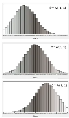
way to evaluate the goodness-of-fit of the IRT analysis. The simulation study employed 9 test lengths (i = 20, 30, 40, 50, 60, 70, 80, 90, and 100 items), 50 sample sizes (N = 20 to 1,000 examinees, with a step of 20), and 3 groups of examinees with ability levels of differing distributional characteristics. The first group comprised of medium ability level examinees, while the majority of examinees in the
second and third group were of low and high ability level, respectively (Fig. 1).
θ ~ N(-1, 1)
θ ~ N(0, 1)
θ ~ N(1, 1)
Figure 1. The ability level distributions for the three groups of the simulation study.
The values for the item difficulty parameter (b) were randomly selected from a standard normal distribution with mean μ = 0 and standard deviation σ = 1, bN(0, 1). As for the values for the discrimination (α) and the guessing (c) parameters, these were randomly sampled from a lognormal distribution α log-N(0, 0.5), and a beta distribution c Β(2, 19), respectively. The value for each quality index was computed as the average over 10 iterations of the IRT analysis, with all parameters being re-estimated every time. Since a highly accurate estimation of those indices was not the primary goal of the present study, the aforementioned amount of iterations was considered adequate. The total number of performed IRT analyses was 13,500 (3 groups x 10 iterations x 50 sample sizes x 9 test lengths).
IV. SIMULATION STUDY PROCESS
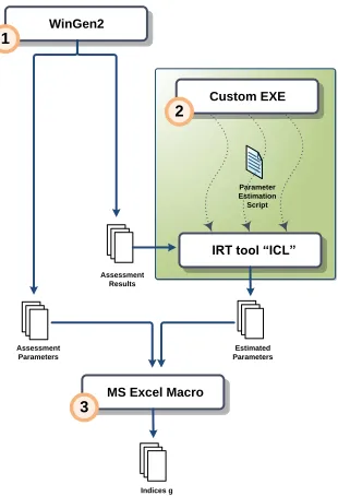
The methodology used in the simulation study can be divided into three steps (Fig. 2).
the true values of the α, b, and c parameters, respectively. Finally, WinGen2 produced and saved the results of the previous test in a new text file with a size of 1000 lines (number of examinees) x 100 columns (total test items) (Fig. 5). Since the IRT model used in the simulation was dichotomous, the only possible answers to the test items were 0 (wrong) and 1 (correct).
Step 2: With the “true” values of the IRT parameters already at hand, the next step was to create their corresponding estimates. For that purpose, a custom Visual Basic program executed ICL for a total number of 1,350 times (3 groups x 50 sample sizes x 9 test lengths), feeding it each time with the simulated response data from WinGen2. Accordingly, ICL performed dichotomous 3PL IRT analysis on the aforementioned data using the following script:
output -no_print
allocate_items_dist <items>
read_examinees out_examinees_<items>.dat
{@11 <items>i1}
starting_values_dichotomous
set fileID [open out_items__<items>
_examinees_<examinees>_results.par w]
write_item_param_channel $fileID -format
%.5e
close $fileID
release_items_dist
Step 3: The resulting file (“out_items_<items>_
examinees_<examinees>_results.par”) was
finally sent to Microsoft Excel in order to calculate the quality indices (gα(0.5), gb(-1.7), gb(1.7), gc(0.2), gαL(10%),
gbL(10%), gbU(10%), gcU(10%)) for that particular pair of items
and examinees.
Parameter Estimation Script
Assessment Results WinGen2
MS Excel Macro
Custom EXE
IRT tool “ICL”
Assessment Parameters
Estimated Parameters
Indices g
1
2
3
Figure 2. Simulation study process
Figure 3. Generating the first group of 1,000 examinees, θ ~ Ν(0, 1).
Figure 4. Generating 100 test items, α log-N(0, 0.5), b N(0, 1), c Β(2, 19).
α <= (0.5) Items
20 40 60 80 100
40 0,17 0,25 0,34 0,33 0,30 80 0,18 0,30 0,45 0,42 0,41 120 0,37 0,45 0,51 0,48 0,45 160 0,25 0,49 0,53 0,51 0,50 200 0,21 0,46 0,54 0,51 0,50 240 0,20 0,50 0,55 0,56 0,53 280 0,19 0,51 0,61 0,56 0,54 320 0,21 0,50 0,59 0,56 0,54 360 0,32 0,52 0,60 0,57 0,56 400 0,26 0,55 0,62 0,58 0,57 440 0,23 0,55 0,61 0,60 0,57 480 0,24 0,57 0,63 0,60 0,58 520 0,27 0,58 0,62 0,59 0,57 560 0,48 0,57 0,61 0,60 0,59 600 0,49 0,57 0,60 0,60 0,58 640 0,49 0,58 0,61 0,59 0,56 680 0,55 0,59 0,62 0,59 0,57 720 0,60 0,59 0,63 0,60 0,57 760 0,61 0,63 0,62 0,59 0,56 800 0,62 0,61 0,61 0,58 0,57 840 0,55 0,59 0,60 0,58 0,56 880 0,68 0,61 0,60 0,58 0,56 920 0,66 0,60 0,62 0,57 0,56 960 0,74 0,62 0,61 0,58 0,58 1000 0,81 0,64 0,62 0,60 0,58
Ex
am
in
ee
s
α Lower (10%)
Items
20 40 60 80 100
40 0,25 0,23 0,25 0,29 0,29 80 0,30 0,38 0,43 0,44 0,40 120 0,45 0,45 0,48 0,46 0,50 160 0,40 0,53 0,52 0,53 0,50 200 0,45 0,45 0,52 0,50 0,49 240 0,45 0,53 0,53 0,51 0,56 280 0,45 0,58 0,50 0,60 0,64 320 0,50 0,58 0,57 0,63 0,62 360 0,55 0,63 0,63 0,64 0,65 400 0,55 0,63 0,63 0,64 0,64 440 0,50 0,65 0,65 0,65 0,68 480 0,55 0,60 0,60 0,64 0,65 520 0,55 0,58 0,62 0,63 0,68 560 0,65 0,63 0,65 0,65 0,66 600 0,65 0,65 0,67 0,69 0,69 640 0,65 0,65 0,67 0,65 0,70 680 0,70 0,75 0,68 0,69 0,73 720 0,65 0,70 0,68 0,65 0,70 760 0,65 0,70 0,68 0,70 0,73 800 0,70 0,68 0,63 0,70 0,73 840 0,75 0,70 0,72 0,69 0,73 880 0,75 0,73 0,70 0,71 0,75 920 0,70 0,73 0,70 0,70 0,73 960 0,75 0,73 0,70 0,70 0,73 1000 0,80 0,68 0,70 0,71 0,75
E xa m in e e s
b <= (-1.7)
Items
20 40 60 80 100
40 0,42 0,37 0,36 0,53 0,52 80 0,56 0,47 0,55 0,66 0,70 120 0,50 0,53 0,58 0,73 0,67 160 0,65 0,55 0,54 0,66 0,64 200 0,65 0,57 0,57 0,70 0,71 240 0,68 0,61 0,63 0,69 0,69 280 0,50 0,64 0,62 0,60 0,63 320 0,65 0,53 0,74 0,78 0,65 360 0,60 0,57 0,60 0,75 0,68 400 0,65 0,59 0,58 0,75 0,68 440 0,50 0,59 0,60 0,77 0,70 480 0,50 0,58 0,58 0,75 0,76 520 0,36 0,64 0,73 0,79 0,79 560 0,50 0,56 0,68 0,76 0,78 600 0,50 0,73 0,68 0,78 0,76 640 0,50 0,63 0,64 0,76 0,74 680 0,50 0,73 0,64 0,77 0,77 720 0,50 0,73 0,68 0,79 0,77 760 0,50 0,73 0,65 0,76 0,76 800 0,50 0,71 0,63 0,76 0,74 840 0,50 0,71 0,68 0,76 0,76 880 0,50 0,71 0,68 0,79 0,77 920 0,36 0,58 0,70 0,79 0,77 960 0,32 0,58 0,65 0,78 0,78 1000 0,46 0,58 0,61 0,78 0,78
E xa m in e e s
b Lower (10%)
Items
20 40 60 80 100
40 0,45 0,58 0,60 0,63 0,61 80 0,60 0,70 0,63 0,69 0,70 120 0,80 0,75 0,67 0,75 0,73 160 0,80 0,78 0,70 0,73 0,74 200 0,85 0,80 0,70 0,78 0,75 240 0,85 0,75 0,68 0,76 0,76 280 0,85 0,75 0,68 0,80 0,78 320 0,80 0,78 0,68 0,80 0,77 360 0,80 0,75 0,72 0,78 0,77 400 0,80 0,75 0,72 0,78 0,79 440 0,80 0,83 0,70 0,75 0,77 480 0,75 0,80 0,72 0,80 0,81 520 0,75 0,83 0,70 0,76 0,78 560 0,80 0,78 0,72 0,79 0,80 600 0,80 0,80 0,73 0,79 0,80 640 0,80 0,80 0,73 0,80 0,80 680 0,80 0,75 0,70 0,80 0,79 720 0,75 0,75 0,70 0,81 0,81 760 0,75 0,73 0,72 0,80 0,80 800 0,80 0,73 0,70 0,81 0,80 840 0,75 0,73 0,68 0,79 0,80 880 0,75 0,73 0,70 0,79 0,80 920 0,75 0,73 0,67 0,79 0,79 960 0,70 0,75 0,68 0,76 0,78 1000 0,75 0,78 0,67 0,76 0,79
E xa m in e e s (0.5) α
g
10%
αL
g gb ( 1.7) gbL10%
b >= (1.7)
Items
20 40 60 80 100
40 0,25 0,37 0,33 0,41 0,41 80 0,34 0,56 0,40 0,56 0,56 120 0,43 0,61 0,41 0,60 0,60 160 0,47 0,44 0,43 0,55 0,58 200 0,71 0,63 0,47 0,63 0,63 240 0,47 0,44 0,48 0,62 0,66 280 0,47 0,55 0,40 0,65 0,67 320 0,43 0,42 0,37 0,63 0,65 360 0,57 0,59 0,46 0,71 0,69 400 0,57 0,46 0,51 0,64 0,72 440 0,85 0,56 0,48 0,69 0,72 480 0,85 0,59 0,52 0,74 0,75 520 0,85 0,62 0,60 0,78 0,75 560 0,85 0,59 0,51 0,77 0,76 600 0,85 0,58 0,57 0,76 0,77 640 0,85 0,71 0,46 0,71 0,72 680 0,85 0,66 0,52 0,76 0,79 720 0,85 0,66 0,60 0,78 0,81 760 0,85 0,69 0,62 0,80 0,83 800 0,85 0,66 0,62 0,83 0,83 840 0,85 0,66 0,62 0,85 0,82 880 0,85 0,66 0,60 0,79 0,84 920 0,85 0,69 0,60 0,83 0,83 960 0,85 0,82 0,62 0,82 0,82 1000 0,85 0,81 0,70 0,79 0,83
Ex
am
in
ee
s
b Upper (10%)
Items
20 40 60 80 100
40 0,55 0,53 0,48 0,55 0,57 80 0,50 0,63 0,48 0,56 0,59 120 0,60 0,63 0,62 0,66 0,64 160 0,65 0,68 0,65 0,69 0,67 200 0,60 0,68 0,65 0,68 0,66 240 0,60 0,75 0,68 0,69 0,67 280 0,65 0,73 0,67 0,73 0,71 320 0,60 0,78 0,63 0,71 0,67 360 0,65 0,78 0,63 0,71 0,72 400 0,65 0,75 0,70 0,73 0,73 440 0,70 0,75 0,72 0,76 0,77 480 0,70 0,78 0,77 0,78 0,80 520 0,65 0,75 0,77 0,78 0,78 560 0,65 0,78 0,77 0,78 0,79 600 0,70 0,80 0,75 0,78 0,80 640 0,70 0,80 0,77 0,75 0,82 680 0,70 0,78 0,77 0,76 0,82 720 0,70 0,80 0,80 0,76 0,79 760 0,60 0,83 0,78 0,78 0,79 800 0,70 0,80 0,80 0,78 0,80 840 0,65 0,83 0,80 0,83 0,82 880 0,65 0,83 0,83 0,78 0,80 920 0,60 0,80 0,78 0,80 0,81 960 0,65 0,83 0,78 0,79 0,79 1000 0,65 0,83 0,78 0,80 0,81
Ex
am
in
ee
s
c >= (0.2)
Items
20 40 60 80 100
40 0,26 0,30 0,27 0,26 0,26 80 0,31 0,28 0,27 0,26 0,26 120 0,25 0,26 0,27 0,27 0,28 160 0,30 0,28 0,31 0,29 0,28 200 0,28 0,29 0,28 0,28 0,28 240 0,33 0,28 0,30 0,30 0,32 280 0,35 0,29 0,34 0,33 0,32 320 0,28 0,27 0,32 0,31 0,30 360 0,32 0,33 0,34 0,32 0,32 400 0,34 0,35 0,32 0,31 0,32 440 0,31 0,31 0,33 0,33 0,32 480 0,30 0,30 0,31 0,31 0,30 520 0,30 0,30 0,32 0,34 0,29 560 0,28 0,31 0,34 0,32 0,31 600 0,27 0,31 0,35 0,34 0,35 640 0,28 0,32 0,37 0,33 0,33 680 0,29 0,30 0,36 0,35 0,34 720 0,31 0,27 0,33 0,34 0,32 760 0,34 0,29 0,34 0,33 0,33 800 0,30 0,27 0,35 0,30 0,31 840 0,34 0,24 0,34 0,30 0,30 880 0,23 0,36 0,36 0,32 0,32 920 0,24 0,36 0,35 0,30 0,32 960 0,10 0,37 0,33 0,29 0,30 1000 0,10 0,30 0,32 0,32 0,28
E xa m in e e s
c Upper (10%)
Items
20 40 60 80 100
40 0,20 0,13 0,12 0,15 0,16 80 0,25 0,25 0,20 0,16 0,18 120 0,20 0,25 0,18 0,21 0,20 160 0,30 0,25 0,27 0,25 0,25 200 0,30 0,28 0,28 0,20 0,18 240 0,25 0,30 0,28 0,25 0,24 280 0,15 0,30 0,32 0,29 0,29 320 0,10 0,28 0,32 0,26 0,28 360 0,15 0,18 0,27 0,30 0,26 400 0,25 0,20 0,33 0,30 0,27 440 0,20 0,25 0,30 0,30 0,28 480 0,20 0,28 0,27 0,26 0,25 520 0,10 0,20 0,25 0,24 0,25 560 0,20 0,25 0,22 0,24 0,26 600 0,20 0,20 0,28 0,25 0,24 640 0,20 0,15 0,32 0,24 0,26 680 0,10 0,18 0,27 0,24 0,26 720 0,20 0,18 0,28 0,25 0,25 760 0,20 0,13 0,35 0,25 0,22 800 0,20 0,23 0,28 0,25 0,23 840 0,20 0,20 0,33 0,26 0,26 880 0,20 0,18 0,35 0,30 0,26 920 0,10 0,25 0,30 0,25 0,28 960 0,05 0,23 0,30 0,25 0,28 1000 0,10 0,23 0,30 0,26 0,25
E xa m in e e s (1.7)
gb gbU10% gc(0.2) gcU10%
0,00 0,10 0,20 0,30 0,40 0,50 0,60 0,70 0,80 0,90 1,00
20 100 180 260 340 420 500 580 660 740 820 900 980
g α (< =0 .5 ) Examinees items 20 30 40 50 60 70 80 90 100 0,00 0,10 0,20 0,30 0,40 0,50 0,60 0,70 0,80 0,90 1,00
20 100 180 260 340 420 500 580 660 740 820 900 980
g α L (1 0 % ) Examinees items 20 30 40 50 60 70 80 90 100 (0.5) α
g gαL10%
0,00 0,10 0,20 0,30 0,40 0,50 0,60 0,70 0,80 0,90 1,00
20 100 180 260 340 420 500 580 660 740 820 900 980
g b (< = -1 .7 ) Examinees items 20 30 40 50 60 70 80 90 100 0,00 0,10 0,20 0,30 0,40 0,50 0,60 0,70 0,80 0,90 1,00
20 100 180 260 340 420 500 580 660 740 820 900 980
g b L (1 0 % ) Examinees items 20 30 40 50 60 70 80 90 100 ( 1.7)
gb
10% L gb 0,00 0,10 0,20 0,30 0,40 0,50 0,60 0,70 0,80 0,90 1,00
20 100 180 260 340 420 500 580 660 740 820 900 980
g b (> = 1 .7 ) Examinees items 20 30 40 50 60 70 80 90 100 0,00 0,10 0,20 0,30 0,40 0,50 0,60 0,70 0,80 0,90 1,00
20 100 180 260 340 420 500 580 660 740 820 900 980
g b U (1 0 % ) Examinees items 20 30 40 50 60 70 80 90 100 (1.7)
gb gbU10%
0,00 0,10 0,20 0,30 0,40 0,50 0,60 0,70 0,80 0,90 1,00
20 100 180 260 340 420 500 580 660 740 820 900 980
g c (> = 0 .2 ) Examinees items 20 30 40 50 60 70 80 90 100 0,00 0,10 0,20 0,30 0,40 0,50 0,60 0,70 0,80 0,90 1,00
20 100 180 260 340 420 500 580 660 740 820 900 980
g c U (1 0 % ) Examinees items 20 30 40 50 60 70 80 90 100 (0.2)
gc
10% U
gc
0,00 0,10 0,20 0,30 0,40 0,50 0,60 0,70 0,80 0,90 1,00
20 100 180 260 340 420 500 580 660 740 820 900 980
g α (< =0 .5 ) Examinees items 20 30 40 50 60 70 80 90 100 0,00 0,10 0,20 0,30 0,40 0,50 0,60 0,70 0,80 0,90 1,00
20 100 180 260 340 420 500 580 660 740 820 900 980
g α L (1 0 % ) Examinees items 20 30 40 50 60 70 80 90 100 (0.5) α
g gαL10%
0,00 0,10 0,20 0,30 0,40 0,50 0,60 0,70 0,80 0,90 1,00
20 100 180 260 340 420 500 580 660 740 820 900 980
g b (< = -1 .7 ) Examinees items 20 30 40 50 60 70 80 90 100 0,00 0,10 0,20 0,30 0,40 0,50 0,60 0,70 0,80 0,90 1,00
20 100 180 260 340 420 500 580 660 740 820 900 980
g b L (1 0 % ) Examinees items 20 30 40 50 60 70 80 90 100 ( 1.7)
gb gbL10%
0,00 0,10 0,20 0,30 0,40 0,50 0,60 0,70 0,80 0,90 1,00
20 100 180 260 340 420 500 580 660 740 820 900 980
g b (> = 1 .7 ) Examinees items 20 30 40 50 60 70 80 90 100 0,00 0,10 0,20 0,30 0,40 0,50 0,60 0,70 0,80 0,90 1,00
20 100 180 260 340 420 500 580 660 740 820 900 980
g b U (1 0 % ) Examinees items 20 30 40 50 60 70 80 90 100 (1.7)
gb gbU10%
0,00 0,10 0,20 0,30 0,40 0,50 0,60 0,70 0,80 0,90 1,00
20 100 180 260 340 420 500 580 660 740 820 900 980
g c (> = 0 .2 ) Examinees items 20 30 40 50 60 70 80 90 100 0,00 0,10 0,20 0,30 0,40 0,50 0,60 0,70 0,80 0,90 1,00
20 100 180 260 340 420 500 580 660 740 820 900 980
g c U (1 0 % ) Examinees items 20 30 40 50 60 70 80 90 100 (0.2)
gc
10% U
gc
0,00 0,10 0,20 0,30 0,40 0,50 0,60 0,70 0,80 0,90 1,00
20 100 180 260 340 420 500 580 660 740 820 900 980
g α (< =0 .5 ) Examinees items 20 30 40 50 60 70 80 90 100 0,00 0,10 0,20 0,30 0,40 0,50 0,60 0,70 0,80 0,90 1,00
20 100 180 260 340 420 500 580 660 740 820 900 980
g α L (1 0 % ) Examinees items 20 30 40 50 60 70 80 90 100 (0.5) α
g gαL10%
0,00 0,10 0,20 0,30 0,40 0,50 0,60 0,70 0,80 0,90 1,00
20 100 180 260 340 420 500 580 660 740 820 900 980
g b (< = -1 .7 ) Examinees items 20 30 40 50 60 70 80 90 100 0,00 0,10 0,20 0,30 0,40 0,50 0,60 0,70 0,80 0,90 1,00
20 100 180 260 340 420 500 580 660 740 820 900 980
g b L (1 0 % ) Examinees items 20 30 40 50 60 70 80 90 100 ( 1.7)
gb
10% L gb 0,00 0,10 0,20 0,30 0,40 0,50 0,60 0,70 0,80 0,90 1,00
20 100 180 260 340 420 500 580 660 740 820 900 980
g b (> = 1 .7 ) Examinees items 20 30 40 50 60 70 80 90 100 0,00 0,10 0,20 0,30 0,40 0,50 0,60 0,70 0,80 0,90 1,00
20 100 180 260 340 420 500 580 660 740 820 900 980
g b U (1 0 % ) Examinees items 20 30 40 50 60 70 80 90 100 (1.7)
gb gbU10%
0,00 0,10 0,20 0,30 0,40 0,50 0,60 0,70 0,80 0,90 1,00
20 100 180 260 340 420 500 580 660 740 820 900 980
g c (> = 0 .2 ) Examinees items 20 30 40 50 60 70 80 90 100 0,00 0,10 0,20 0,30 0,40 0,50 0,60 0,70 0,80 0,90 1,00
20 100 180 260 340 420 500 580 660 740 820 900 980
g c U (1 0 % ) Examinees items 20 30 40 50 60 70 80 90 100 (0.2)
gc gcU10%
V. RESULTS -DISCUSSION
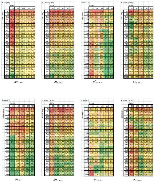
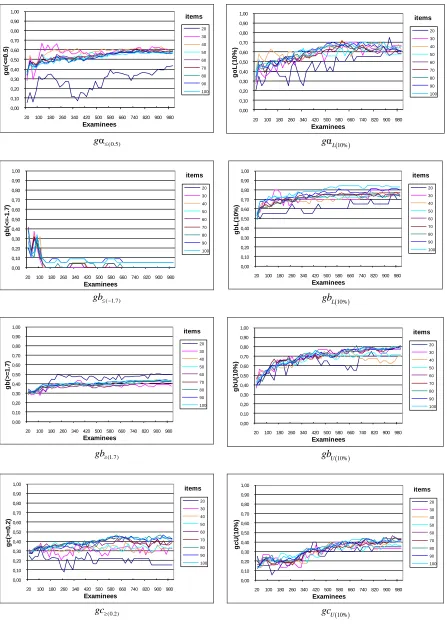
Indices gα(0.5), gb(-1.7), gb(1.7), gc(0.2), gαL(10%), gbL(10%),
gbU(10%), and gcU(10%) can be practically treated as indicators
of the IRT analysis success rate. For instance, according to the first group simulation (examinees with ability parameters θ ~ Ν(0,1)), the value for index gbL(10%) in a
sample of 30 items and 160 examinees is 0.70. This can be interpreted as follows: when performing an IRT analysis to detect the 3 lowest difficulty items (i.e., 10% of the 30 items), only 2 of the results (i.e., 66% 70%) will be among the actual items with the lowest difficulty.
In the same manner, index gb(1.7) receives the value of
0.71 in a sample of 80 items and 360 examinees (Fig. 6). In practice this means that, if the IRT analysis returns 5 items when asked to identify which ones have the highest difficulty level (b ≥ 1.7), only 4 of them (71% of the 5 items = 3.55 4) will, in fact, be among the ones with the highest difficulty.
As can be seen in Fig. 10a, the best fit between estimated and actual values for parameter b in a 100-item assessment test is achieved when the ability level of the examinees is medium, i.e., θ ~ Ν(0, 1). The measured Root Mean Square Error (RMSE) is considerably larger in the case of examinees with high ability levels θ ~ Ν(1, 1), and increases even further when the majority of examinees are of low ability (θ ~ Ν(-1, 1)). Nevertheless, the probability of an item identified by the IRT analysis as being very difficult to be among the actual items with the highest degree of difficulty remains virtually the same for all three cases, regardless of the examinees' ability level (Fig. 10b).
0,00 0,10 0,20 0,30 0,40 0,50 0,60 0,70 0,80 0,90 1,00
20 180 340 500 660 820 980
g
bU(1
0
%)
Examinees 100 items
θ~N(-1,1)
θ~N(1,1)
θ~N(0,1) 0,00
0,50 1,00 1,50 2,00
20 180 340 500 660 820 980
RMS
E
(
b
)
Examinees 100 items
θ~N(-1,1)
θ~N(1,1)
θ~N(0,1)
(a)
(b)
Figure 10. A comparison between (a) the fit index Root Mean Square Error (RMSE), and (b) the proposed quality index gbU(10%) for the b parameter.
Consequently, despite the fact that the estimated values for parameter b are cohort-dependent, the ranking of those values is independent of cohort type and remains unchanged. Based on the above observations, it can be concluded that the proposed indices represent a practical and reliable means of assessing the quality of the IRT analysis results.
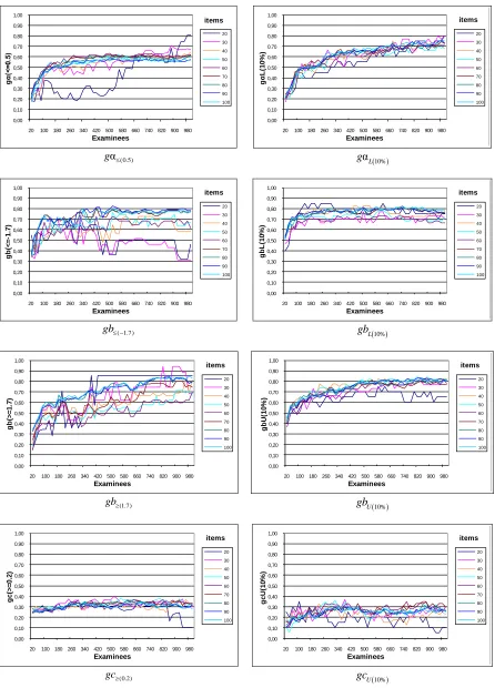
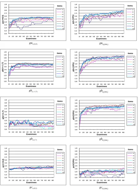
According to Fig. 8, IRT analysis fails to produce satisfactory results when attempting to detect items with low level of difficulty (b -1.7) in the case of the low-ability cohort (θ ~ Ν(-1, 1)), i.e., the success rate denoted by index
gb(-1.7) is considerably low. However, this finding was to be
expected, since most low ability examinees may experience considerable problems when trying to answer all questions, including low difficulty ones. In spite of this, index gbL(10%)
appears unaffected by the cohort's ability level and, consequently, does not change. The explanation lies in the fact that there is still a match in the order of the actual and their corresponding estimated parameters, despite the poor item fit caused by small sample sizes.
Similarly, IRT analysis produces poor results when attempting to detect items with a high level of difficulty (b ≥ 1.7) in the case of the high-ability cohort (θ ~ Ν(1, 1)), i.e., the success rate provided by index gb(1.7) is low (Fig. 9).
This finding was equally unsurprising since most high ability examinees may answer most, perhaps all, questions correctly regardless of their actual difficulty level. Once again, the corresponding index gbU(10%) appears unaffected
by the cohort's ability level and does not change.
Overall, the IRT analysis results seemed unaffected by the different distributions associated with examinees’ ability levels; the only exception to this rule was a decrease in the performance of indices gb(-1.7) and gb(1.7) for groups with θ
~ Ν(-1, 1) and θ ~ Ν(1, 1), respectively. This, in conjunction with the fact that indices gαL(10%), gbL(10%), gbU(10%), and
gcU(10%) perform better than gα(0.5), gb(-1.7), gb(1.7), and
gc(0.2) suggests that it would be best to base the methods
used to detect flawed items not on specific parameter values, but on ranges near boundaries.
Finally, the values displayed in Fig. 6 are largely dependent on the distributions of both θ and the item parameters as generated by WinGen2. These parameters were specifically selected with the aim of simulating realistic item response data so as to produce reliable results. However, further experiments exceeding the scope of the present study have revealed that an increase in the mean of the distribution of the guessing parameter c would also result in a considerable decline in performance.
VI. CONCLUSIONS AND FUTURE WORK
Even though research focused on IRT sample size effects suggests that more than 1,000 examinees are needed
to obtain accurate results when using the 3PL model [44], the simulated data depicted in Fig. 6 show that a sample of only 100 examinees can produce relatively satisfying results (gbL(10%) = 0.7) when trying to detect defective items with a
low level of difficulty (gbL(10%)). In cases of assessments
examinees. Attempts to detect items with a high level of difficulty (gbU(10%)) have proven equally encouraging, with
success rates exceeding 70% for sample sizes of 260 examinees and above.
Nevertheless, as the number of examinees is reduced from 200 to 100 and finally down to 20, the success rate of potentially flawed items detection drops dramatically (Fig. 7, 8, 9). Since all indices perform rather poorly for a sample of 50 examinees (< 30%), it becomes obvious that a smaller sample will produce even less adequate results. Therefore, addressing the scenario of a set comprised of less than 20 examinees deemed unnecessary for the purpose of the present study.
As expected given the small size of the samples described above, parameter b appears to be estimated more accurately than parameters α and c. However, in order to achieve an acceptable degree of success when trying to detect items with low discrimination (parameter α) the required number of examinees exceeds the 660 mark. In addition, even a sample size as large as 1,000 seems insufficient to produce reliable estimates for parameter c. These findings indicate that in academic contexts where the sample size can roughly exceed 120 examinees, IRT-based assessment could in practice be used only to identify inappropriate items according to their level of difficulty. In any other case, this procedure has the risk of losing the measurement precision, as well as other advantages of IRT. Further investigation into the impact of sample size on IRT assessment is needed and will be undertaken by performing a greater number of simulations in the near future.
REFERENCES
[1] P. Fotaris, T. Mastoras, I. Mavridis, and A. Manitsaris, “Performance Evaluation of the Small Sample Dichotomous IRT Analysis in Assessment Calibration,” Proc. Fifth International Multi-conference on Computing in the Global Information Technology ICCGI 2010, Valencia, Spain, Sep. 2010, pp. 214-219.
[2] V. S. Anantatmula and M. Stankosky, “KM criteria for different types of organisations,” International Journal of Knowledge and Learning, vol. 4, no. 1, 2008, pp. 18-35, doi:10.1504/IJKL.2008.019735. [3] H. Rego, T. Moreira, F. Garcia, and E. Morales, “Metadata and
knowledge management driven web-based learning information system,” International Journal of Technology Enhanced Learning, vol. 1, no. 3, 2009, pp. 215-228, doi:10.1504/IJTEL.2009.024868. [4] S. Virtanen, “Increasing the self-study effort of higher education
engineering students with an online learning platform,” International Journal of Knowledge and Learning, vol. 4, no. 6, 2009, pp. 527-538, doi:10.1504/IJKL.2008.022886.
[5] G. Baggott and R. Rayne, “Learning Support for Mature, Part-time, Evening Students: Providing Feedback via Frequent, Computer-Based Assessments,” Proc. Fifth International Computer Assisted Assessment Conference, Loughborough University, Jul. 2001, pp. 9-20.
[6] J. Dalziel, “Enhancing Web-Based Learning with Computer Assisted Assessment: Pedagogical and Technical Considerations,” Proc. Fifth International Computer Assisted Assessment Conference, Loughborough University, Jul. 2001, pp. 99-107.
[7] P. Davies, “Computer Aided Assessment MUST be more than Multiple-Choice Tests for it to be Academically Credible?” Proc. Fifth International Computer Assisted Assessment Conference, Loughborough University, Jul. 2001, pp. 143-150.
[8] G. Lambert, “What is Computer Aided Assessment and how can I use it in my teaching,” 2004, [online], Available:
http://www.canterbury.ac.uk/Support/learning-teaching-
enhancement-unit/Resources/Documents/BriefingNotes/Blackboard.pdf, [Accessed 15th January 2011].
[9] U. P. Singh and M. R. de Villiers, “Establishing the current extent and nature of usage of Online Assessment Tools in Computing-related Departments at South African Tertiary Institutions,” Proc. SACLA 2010, Zebra Country Lodge, Jun. 2010.
[10] G. Brown, J. Bull, and M. Pendlebury, Assessing Student Learning in Higher Education, London: Routledge, 1997.
[11] D. Boud, Enhancing learning through self assessment, London: Rutledge, 1995.
[12] J. Wood and M. Burrow, “Formative Assessment in Engineering Using "TRIADS" Software,” Proc. of the Sixth International Computer Assisted Assessment Conference, Loughborough University, 2002, pp.369-380.
[13] T. M. Haladyna, Developing and Validating Multiple-Choice Test Items, 2nd ed., Mahwah, NJ: Lawrence Erlbaum Associates, 1999. [14] SCOREPAK: Item Analysis, unpublished.
[15] F. M. Lord, Applications of Item Response Theory to Practical Testing Problems, Hillsdale, NJ: Lawrence Erlbaum Associates, 1980.
[16] R. E. Bennett and D. H. Gitomer, “Transforming K–12 assessment: Integrating accountability testing, formative assessment, and professional support,” in Educational assessment in the 21st century,
C. Wyatt‐Smith and J. Cumming, Eds. New York: Springer, 2009, pp. 43–61.
[17] C. Spearman, “General intelligence: Objectively determined and measured,” American Journal of Psychology, vol. 15, 1904, pp. 201– 293.
[18] R. K. Hambleton and R. W. Jones, “Comparison of Classical Test Theory and Item Response Theory and their Applications to Test Development,” Educational Measurement: Issues and Practices, vol. 12, 1993 pp. 38-46, doi:10.1111/j.1745-3992.1993.tb00543.x [19] R. K. Hambleton, “Principles and selected applications of item
response theory,” in Educational measurement, 3rd ed., R. L. Linn,
Ed., New York: Macmillan, 1989, pp. 147-200.
[20] R. K. Hambleton and H. Swaminathan, Item Response Theory: Principles and Applications, Boston, MA: Kluwer-Nijhoff Publishing, 1987.
[21] C. B. Schmeiser and C. J. Welch, “Test Development,” in Educational Measurement 4th ed., in R. .L. Brennan, ed. Westport, CT: Praeger Publishers, 2006.
[22] X. Fan, “Item response theory and classical test theory: An empirical comparison of their item/person parameters,” Educational and Psychological Measurement, vol. 58, 1998, pp. 357–381.
[23] Š. Progar and G. Sočan, “An empirical comparison of Item Response Theory and Classical Test Theory,” Horizons of Psychology, vol. 17, no. 3, 2008, pp. 5–24.
[24] A. Birnbaum, “Some Latent Trait Models and their Use in Inferring an Examinee’s Ability,”, in Statistical Theories of Mental Test Scores, F. M. Lord and M. R. Novick, Eds. Reading: Addison-Wesley, 1968.
[25] G. Rasch, Probabilistic models for some intelligence and attainment tests, Copenhagen, Denmark: Danmarks Paedogogische Institut, 1960.
[26] F. B. Baker, Item Response Theory: Parameter Estimation Techniques, New York:Marcel Dekker, 1992, doi:10.2307/2532822 [27] R. K. Hambleton, H. Swaminathan, and H. J. Rogers, Fundamentals
of item response theory. Newbury Park, CA: Sage, 1991.
[29] S. M. Downing, “Item response theory: applications of modern test theory in medical education,” Medical Education, vol. 37, no. 8, 2003, pp. 739-745, doi:10.1046/j.1365-2923.2003.01587.x.
[30] B. D. Wright and M. H. Stone, Best Test Design, Chicago: MESA Press, 1979.
[31] M. D. Reckase, “Unifactor latent trait models applied to multi-factor tests: Results and implications,” Journal of Educational Statistics, vol. 4, 1979, pp. 207-230.
[32] B. B. Reeve and P. Fayer, “Applying item response theory modelling for evaluating questionnaire item and scale properties,” in Assessing quality of life in clinical trials, 2nd ed., P. Fayers and R. Hays, Eds. Oxford: Oxford University Press, 2005.
[33] J. M. Linacre, “Sample size and item calibration stability,” Rasch Measurement Transactions, vol. 37 no. 4, 1994, p. 328.
[34] P. Fotaris, T. Mastoras, I. Mavridis and A. Manitsaris, “Extending LMS to Support IRT-Based Assessment Test Calibration,” in Technology Enhanced Learning. Quality of Teaching and Educational Reform, M. D. Lytras et al., Eds. vol. 73, Berlin Heidelberg: Springer, pp. 534-543.
[35] W. M. Yen and A. R. Fitzpatrick, “Item Response Theory,” in Educational Measurement 4th ed., in R. .L. Brennan, ed. Westport, CT: Praeger Publishers, 2006.
[36] M. Orlando and D. Thissen, “New item fit indices for dichotomous item response theory models,” Applied Psychological Measurement, vol. 24, 2000, pp. 50-64.
[37] M. Orlando and D. Thissen, “Further investigation of the performance of S-X2: An item fit index for use with dichotomous item response theory models,” Applied Psychological Measurement, vol. 27, 2003, pp. 289-298, doi:10.1177/0146621603027004004.
[38] W. M. Yen, “Using simulation results to choose a latent trait model,” Applied Psychological Measurement, vol. 5, 1981, pp. 245-262, doi:10.1177/014662168100500212.
[39] R. L. McKinley and C. N. Mills, “A comparison of several goodness-of-fit statistics,” Applied Psychological Measurement, vol. 9, 1985, pp. 49-57, doi:10.1177/014662168500900105.
[40] K. T. Han, “WinGen: Windows Software That Generates Item Response Theory Parameters and Item Responses,” Applied Psychological Measurement, vol. 31, no.5, Sept. 2007, pp. 457-459, doi: 10.1177/0146621607299271.
[41] B. A. Hanson, IRT Command Language (ICL), unpublished. [42] B. B. Welch, K. Jones, and J. Hobbs, Practical programming in Tcl
and Tk, 4th ed., Upper Saddle River, NJ: Prentice Hall, 2003. [43] R. Flaugher, “Item Pools,” in Computerized Adaptive Testing: A
Primer, 2nd ed., H. Wainer, Ed. Mahwah, NJ: Lawrence Erlbaum Associates, 2000.