Transmission Power and Effects on Energy Consumption
and Performance in MANET
S. Blakeway
1*, A. Kirpichnikova
2, M. Schaeffer
3, E.L. Secco
41Faculty of Science and Engineering, School of Computer Science, University of Manchester, UK
2Department of Computing Science and Mathematics, University of Stirling, UK
3Institut National Des Sciences Appliquees, INSA, France
4Robotic Laboratory, Department of Mathematics & Computer Science, Liverpool Hope University, Hope Park L16 9JD, UK
Abstract
This paper explores the effect that transmission power has on the performance of a Mobile Ad hoc Network (MANET). The goal of this research is to determine if the lifetime of the network can be prolongated by using less energy and thus, resulting in a more energy efficient ‘greener’ architecture. A total of 72 unique simulations are conducted of various configurations covering a large variety of possible scenarios: we examined configurations with a different number of nodes, number of traffic flows, mobility model, transmission power and geographical areas. Results show that there is an optimal transmission power, which enhances greater network performance: moreover, this optimal transmission setting makes the network more energy efficient in terms of depletion of the finite energy sources of the nodes. Our overall findings also confirm that higher transmission power results in less energy consumption
Keywords: MANET, Green Networks, Transmission Power Optimization, Energy Aware Networks.
Received on DD MM YYYY, accepted on DD MM YYYY, published on DD MM YYYY
Copyright © YYYY Author et al., licensed to EAI. This is an open access article distributed under the terms of the Creative Commons Attribution licence (http://creativecommons.org/licenses/by/3.0/), which permits unlimited use, distribution and reproduction in any medium so long as the original work is properly cited.
doi: _______________
1. Introduction
There has been much research of TPCPs (Transmission Power Control Protocols) in recent years, for example in an empirical study was conducted to determine a target TP (Transmission Power) based on an optimum TP [1]. The optimum TP was obtained using three link control properties and empirical data. In our research, we also consider one of the link control properties discussed which is that of Packet Delivery. We also consider the other link properties (Channel Quality and Channel Stability) but we do so transitively, i.e. based on the packet delivery ratio, if packets are being delivered it can be assumed that both Channel Quality and Channel Stability are sufficiently high for the successful transmission of data packets.
Authors in [2] give explanations to quantify the energy dissipated by the transmitting and receiving antennas and they describe the Heinselman-Chandrakasan-Balakrishnan (HCB) energy model [3]. Moreover, the authors of paper [2] give metrics of the power drain properties of
state-of-the art radio antenna design. In our research, a Wi-fi Radio Energy Model was used that defines 4 states TX, RX, IDLE and SLEEP. The default state being IDLE. The different types of transactions that are defined are detailed in [4]. The default values for power consumption are based on measurements reported in [5] and are discussed in more detail in the methodology.
There has been research conducted that detail the issues of selecting the transmission power in order to minimize the transmission power and thus conserve energy [6]. The work calculates the transmission power required to transmit n number of bits (which are converted to energy). The authors explain how the automatic repeat request (ARQ) protocol was used to establish link quality. The work also incorporates error percentage of the expected energy levels.
network. Our work also differs because we are using a MANET whereby their work considered static sensor networks (two topologies). Unfortunately, it was unclear which simulation software was used and the other configuration parameters for their experiments. However, their results are promising and show that there is not a significant trade-off between performance and scaling up the transmission power. Also, mentioned in the future work section was that one may consider other routing protocols such as Ad hoc On-Demand Distance Vector (AODV), our research uses this routing protocol as well as the Destination-Sequenced Distance-Vector (DSDV).
Other related work has been conducted in [8] whereby authors considered energy consumption in sensor networks like that of the work of [7]. The authors explain that transmitting at a constant highest transmission power leads to energy wastage and causes interference. The simulations conducted using Castalia simulator show that by using a closed loop feedback system that the system can reduce the energy consumption of the nodes without compromising packet receive rates. Although similar to our work and the work in [7] the author in [8] designed a microcontroller to run the algorithm that contains the closed control loop. Our work differs for the reasons given previously, we are simulating energy in a network with a volatile topology.
The above is key and currently literature in relations to reducing the transmission power to save energy. Notwithstanding the different reasons for saving energy, it agrees with all research reviewed that saving energy is of great importance. Different approaches have been made to tackling this area of research, for example in [1] an empirical model was used, in [2] authors focused more on the characteristics of antennas and power consumption. In [6] authors were interested with determining the link quality and number of bits to transmit to determine the transmission power. In [7] the authors focused on two sensor networks and altered the transmission power and analyzed the performance of the network. Work published in [8] is like that of [7] but authors of [8] discuss a hardware implementation to their solution.
This research applies power saving techniques to a Mobile Ad Hoc Network (MANET) to prolong the lifetime of that network. A MANET is a packet switching data communications network that operates without a predefined infrastructure. The nodes within a MANET communicate using wireless technology and transmit radio waves omnidirectionally. These radio waves are received by all nodes within the transmission range of the sender. To communicate with a node that is not within the senders’ transmission range, the nodes that are within range of the sender will forward the packet on behalf of the sender, therefore, a node within a MANET also takes on the additional responsibility of routing and forwarding packets. There are many applications for a MANET which range from personal area networks (PANs) to large scale Wide Area Networks (WANs) that could potentially span over many miles [9]. There are also many application areas, for example, Vehicular ad hoc networks (VANETs) and Smart phone ad hoc networks (SPANs). The application that this
research considers is that of Disaster rescue ad hoc networks [10]. Disaster recovery could be a result of a natural catastrophe, such as a landslide or sinkhole, or it could be because of a malicious attack such as a bomb, or there could have been some form of accident such as a fire. It is essential in these situations to establish a communications infrastructure with the intention to coordinate efforts which may potentially save lives.
Due to the critical application area, it is not only important to establish communications quickly, but it is also important to maintain communications. Due to the nature of the nodes being mobile, the nodes are normally equipped with a finite energy source, for example, a lithium battery. It is important for the network to be as efficient as possible in terms of energy depletion of the nodes.
Energy consumption in a MANET has been a focus of research in recent years [11,13] and many authors have looked at ways to improve the power consumption by optimizing the performance of routing protocols [12,14] or by managing the flow of packets using sliding windows and buffers [15]. Thus, much of the research in energy is conducted at the network layer.
This research optimizes energy consumption by using a cross-layered approach and reduces power-output at the physical layer by dynamically reducing the transmission and reception power of the antennas of the nodes. This approach was taken because of the broadcast nature of a MANET, that is, when a packet is sent all nodes within communications range of the source node will receive that packet and process the packet, even when they are not the intended recipient. In addition to this larger transmission areas could result in media contention issues and congestion which delays the sending of packets.
The theoretical design presented in this manuscript was implemented in Network Simulator 3 and consists of several simulations ranging from areas of low density to areas of high density. In all the simulations run the life-time of the network was increased with little or no consequence in relation to packet delivery rate.
The remainder of this manuscript is organized as follows. In the Materials and Methods section, we define the simulation parameters with justification for these. The results section clearly shows a correlation between transmission/reception power and the life-time of the communications network, whilst still maintaining a quality of service. The discussion section details the findings of this research and offers insight for the results. The conclusion summaries the findings and discusses potential future work.
2. Materials and Methods
doubled to 18, these are also placed in a grid formation.
Scenario 2 also utilized multiple sources and destinations, node 0 transmits to node 14 and node 4 transmits to node 17. Each of the scenarios contained three types of configuration (a, b and c), the first configuration (a), nodes were fixed and did not move position, the second configuration (b) the Random Waypoint Mobility Model (RWP) is applied, the third configuration (c) dynamically altered transmission power whilst the simulation was running. All simulations ran for 500 s except for configuration c, which ran for 504 s. Table 1 summarizes the general configurations.
Scenarios
1A 1B 1C 2A 2B 2C
Number of
Nodes 9 18
Number of Power Levels
21 14 21
Geographic
al Area 200 x 200 m 500 x 200 m
Mobility
Model C RWP C C RWP C
Simulation
Time 500 s 504 s 500 s 504 s
Table 1. Summary of the Scenarios (C refers to a
Constant mobility model).
2.1 Nodes
In the context of MANET, a node is any device that has to capability of transmitting and receiving radio signals. In
Scenario 1 the number of nodes participating in the network is 9, in Scenario 2 the number of nodes is doubled to 18, see Figure 1 for an illustration of the increase in number of nodes for each scenario and the increase in geographical area, the image is a screen capture from Network Animator (NetAnim) and the nodes are represented by red circles. In Figure 1, the left topology shows a point in time before transmission has begun, the right topology shows transmission between the nodes is occurring and is represented by blue directional lines.
2.2 Network Animators
NetAnim (Network Animator) version 3.108, is bundled with Network Simulator 3 version 3.27, and is a sophisticated visualisation tool. The NetAnim graphical user interface allows the animation of packets propagating over both wired and wireless links. NetAnim also supports Visualisation for packet timelines, the ability to see the node position(s) at a given point in time (including node
trajectory), plus more features including but not limited to routing tables at various times for the node(s).
Figure 1. The 3x3 and 6x3 Network Topologies on the top and bottom panels, respectively.
2.3 Antennas, Transmission and Energy
Sources
At the Physical (PHY) layer, the nodes were configured to use Direct Sequence Spread Spectrum (DSSS) at a rate of 11 Mbit/s. At the application layer, the packet size was configured to 2048 bits with a data transmit rate of 2048 bit/s. Transmission mode for non-unicast data frames was also set to DSSS. The wireless standard used in the simulations is the IEEE 802.11b. A constant speed propagation delay model was applied with the default propagation speed of light in a vacuum measured in meters per second (m/s) or 299,792,458 m/s. The Friis Propagation Loss Model [16] was used to model propagation loss and is described by the formula:
(
)
2
2
4
t t r
r
P G G
P
d
L
=
Where Pr is the reception power (W), Pt is the transmission power (W), Gt is the transmission gain (unit-less), Gr is the reception gain (unit-less), λ is the wavelength (m), d is the distance (m) and L is the system loss (unit-less).
At the Media Access Control (MAC) layer the constant rate Wi-Fi manager was disabled and the data mode and control mode assigned to the PHY layer. The MAC was also configured for operation in ad hoc mode.
scenario being run the transmission power was set between -10 dB and +10 dB. The transmission power remains constant until the transmission of the packet has ended. The real transmission power is calculated as follows:
𝑇𝑥𝑃𝑜𝑤𝑒𝑟𝑀𝑖𝑛 + 𝑇𝑥𝑃𝑜𝑤𝑒𝑟𝐿𝑒𝑣𝑒𝑙 × 𝑇𝑥𝑃𝑜𝑤𝑒𝑟𝑀𝑎𝑥 − 𝑇𝑥𝑃𝑜𝑤𝑒𝑟𝑀𝑖𝑛 𝑛𝑢𝑚𝑏𝑒𝑟 𝑜𝑓 𝑇𝑥𝐿𝑒𝑣𝑒𝑙𝑠
The other power configuration settings can be found in Table 2.
Configuration Setting
Voltage 3.0 V
Tx Power Start/End -10 dBm to +10 dBm
Number of Tx Power Levels 20 (steps of 1 dB)
Idle Current 0.273 A
TxCurrent 0.389 A
Table 2. The transmission power settings
To transmit a packet, power must be drawn from an independent finite energy source of the node. In each of the simulations an energy source that represents a lithium-ion battery was installed on each node. Lithium-lithium-ion batteries are common in mobile devices such as smart phones and laptops. The initial charge of every battery is 1000 Joules with a supply voltage of 3.0 Volts.
2.4 Node Placement and Mobility Model
The nodes were placed uniformly within the confines of the geographical area for the simulation run. Figure 1 shows initial placement of the nodes. The initial distance between each node for is 100meters. The geographical area of Scenario 2 is double that of Scenario 1 to accommodate more nodes and the initial 100 m distance between the nodes.
Although the nodes were initially placed uniformly, their mobility consisted of random movements, speeds and pause times. The random waypoint mobility model was applied to each node for configurations b, therefore,
Scenario 1b and Scenario 2b allowed the random movement of each node. Each node chooses a waypoint (next leg of journey) using a random value. A random speed is also chosen by each node for each leg of the journey, this was set between 0 m/s and 2.5 m/s (i.e. a maximum speed of 9 km/h) which is in line with the average walking speed. The pause speed (when arriving at each leg of the journey) was set to a constant of 0 seconds, thus the nodes moved continually for the duration of the simulation.
2.5 Routing Protocols
All nodes were configured with the Ad hoc On-Demand Distance Vector (AODV) routing protocol. AODV is a reactive routing protocol and scalable, global routing was
enabled. All nodes interfaces (i.e. network cards) were configured with IP addresses starting at 10.1.1.1 - 10.1.1.n where n is the number of nodes in the simulation + 1. The IP addresses were assigned sequentially. Thus, the node with ID 11 was assigned IP address 10.1.1.12 (node IDs start at 0). The subnet mask assigned was 255.255.255.0 which easily accommodated the number of nodes within the network.
2.6 Traffic Flows
Node 0 was configured to transmit packets to node 8, beginning at 0 s with a constant random variable of 1.0, i.e. from some point between 0.0-1.0 s. Transmission of packets is persistent until the end of the simulation (500 s or 504 s depending on configuration). The nodes used the user datagram protocol (UDP) as the transport protocol and transmitted at a constant bit rate (CBR) of 2048 B/s. A call back (trace) was configured at node 0, which allowed the capturing of sent and received packets, further detail is provided in Section 2.8.
The above describes the traffic flow for Scenario 1 (a, b
and c), for Scenario 2 (a, b and c) an additional traffic flow was configured between node 4 (sender) and node 17 (destination). The same configuration as discussed above was used for this additional traffic flow.
2.7 Transmission and Received Power
The transmission and reception power for configurations a and b for both Scenarios 1 and 2 is configured before the simulation begins and remains constant for the duration of the simulation. Thus, to evaluate network performance for 21 different transmission/reception power levels (-10 dB to +10 dB) 21 distinct and separate simulations were conducted.
Scenario 1c and Scenario 2c used dynamic transmission power levels, i.e. the transmission power dynamically changed as the simulation ran. The transmission power was set to change at intervals of 24 seconds with increments of 1dB per interval. This is the reason that simulations performed with configuration c are slightly longer in duration than 500 s.
2.8 Data Acquisition
Also of interest is the power consumption of the nodes within the network, thus we needed to capture the data associated with the energy sources installed in the nodes. In particular for the nodes involved in the transmitting and receiving of data (the source and the destinations). This allows for analysis to determine if the network lifetime could be prolongated in relation to the transmission power values.
2.8.1 Received Packets
Each time a packet is received by the destination, a packet counter variable is updated by one. At each second of the simulation, throughput is calculated using number of packets captured for that duration. These calculations are stored in a Comma Separated Value (CSV) file. This file also contains the time at which the throughput was calculated, the number of packets received, the number of sinks, which routing protocol was used and the Tx power used to transmit the packet. A snippet of the file is shown in Table 3.
Time Stamp
Receive Rate
Received Packets
Number of Sinks
Routing Protocol
Transmission Power 98.000 0.000 0.000 1 AODV 0.000 99.000 0.000 0.000 1 AODV 0.500 100.000 0.000 0.000 1 AODV 1.000 101.000 10.752 72.000 1 AODV 1.500 102.000 36.864 72.000 1 AODV 2.000 103.000 36.864 72.000 1 AODV 2.500 104.000 36.864 72.000 1 AODV 2.500 118.000 36.864 72.000 1 AODV 2.500 119.000 36.864 72.000 1 AODV 2.500
Table 3. Received Packets according to time stamp, rate of reception, number of received packets and
number of sinks (1st, 2nd, 3rd and 4th columns
respectively).
2.9 Transmitter State and Remaining
Energy
The transmission power is captured in s - microseconds and also when a change to transmission power had occurred, in addition the new power value was captured. To monitor the lifetime of the network we also captured the energy values (i.e. the remaining energy for the energy source) for each and every node, every 5s. All captured data were output to Comma Separated Value (CSV) text files for the analysis in MATLAB (The Mathworks Inc ®), R or other analytical software. The simulation also captured the state of the transmitter continually for each node within the simulation. Figure 2 gives an example of the transmitter state file for node 0. The figure also shows the current simulator time in seconds, the state of the transmitter, when it entered this state and the duration of the state. This assured that the antenna model was operating correctly.
Figure 2. Acquisition of the Transmitter States.
The remaining energy for each node was also captured into a text file. All nodes started out with equal power for their energy sources. The draw on the energy source is dependent on what state the transmitter is in. For example, when in Idle state the current drawn is 0.273 A, but when the transmitter is in Tx (transmitting) state, the current drawn is 0.389 A. The transmission power will influence the current drawn when in Tx state, the higher the transmission power the greater the ampere drawn.
Figure 3. Acquisition of the Mobility States.
2.10 Mobility
The mobility of all the nodes for both Scenarios 1b and
2b was also captured. This data was captured because if something unexpected happened, the position of each of the nodes at a given moment in time could be accertained for analysis. The data captured is time, node identifier, the current position at that time and the velocity of the node. Figure 3 illustrates the format of the data captured. There are two lines per time entry, the second entry shows the nodes trajectory.
2.11 Transmission Power & Distance
To ensure the simulations were running as expected many preliminary simulations were run, 41 of the preliminary simulations that were run each used a different transmission power setting. Each of these simulations consisted of only two nodes which began sufficiently close to one another so that they could communicate (in transmission range). At each second, node 1 would move one meter away from node 0, node 1 continued to do this until communication ceased, this gave a maximum distance for a given transmission power. Table 4 shows the results from these preliminary simulations.
Tx Power DistanceMax Tx Power DistanceMax
-20 12 1 151
-19 14 2 168
-18 16 3 191
-17 18 4 215
-15 23 6 270
-14 25 7 304
-13 30 8 342
-12 33 9 382
-11 38 10 430
-10 42 11 481
-9 47 12 539
-8 52 13 605
-7 59 14 678
-6 66 15 763
-5 75 16 864
-4 85 17 967
-3 96 18 1084
-2 107 19 1215
-1 121 20 1355
0 134
Table 4. The simulation results: TxPower vs
DistanceMax.
Figure 4 depicts the plotted data from Table 4 and shows that nodes can successfully communicate over longer distances by increasing the transmission power.
Figure 4. Transmission Power vs Distance.
Other preliminary simulations allowed the checking of energy sources to ensure that they were being depleted correctly, when an energy source dropped to level that was below a transmission/reception energy threshold the node entered a sleep state and could not transmit or receive further packets.
In addition, traffic flows were checked to ensure they worked as expected and packets were captured correctly. NetAnim also helped verify some other configuration settings such as node placement and mobility. In addition to this live output was observed from the simulator as it ran, this output consisted of all the changes or events of interest that occurred in the simulation.
See Figure 5 which is a capture of an area of the Linux terminal window and depicts the beginning of a simulation run.
2.12 Data Captured for Scenarios 1 and 2
Once convinced by the preliminary simulations that the network was running and capturing data accurately we
tailored the data captured. Data was captured continuously as the simulation ran which resulted in huge data sets. Therefore, because of computational resources we summarized the continuously captured data and output the results to a CSV file every 5 s. Namely the data of interest were; simulation time, the number of sent packets, the number of received packets, the energy depleted, the transmission power, the position of the nodes and the distances between the nodes.
Other data, as described earlier was also captured for further verification but was not used as part of the main analysis, although it provided useful when discussing the analysis to confirm the assumptions made were justified and correct, for example, NetAnim was also configured to capture the animator XML file.
Figure 5. Live output as the simulation runs.
3. Results
Each one of the two scenarios were simulated in three different configurations, namely configuration a, configuration b and configuration c.
Configuration a used a grid placement model and a constant mobility model (the nodes did not move from their original placement positions). Configuration b was a variation of configuration a, but the random waypoint mobility model was applied with restrictive mobility within the original defined geographical areas (Scenario 1, 200 m x 200 m and Scenario 2, 500 m x 200 m). Configuration a and b were run many times, once for each transmission power level being evaluated. In Scenario 1, transmission power was evaluated from -10 dB to +10 dB in steps of 1 dB, thus a total of 21 simulations for each configuration were run. In Scenario 2, the transmission power was evaluated from -3 dB to +10 dB, thus for each configuration a and b, a total of 14 simulations were run.
24 seconds, starting at -10 dB and incrementing in steps of 1 dB to +10 dB. Thus, a range of transmission power levels were tested in two simulations.
In total 72 unique and independent simulations were run, and the data captured (number of sent packets, number of received packets, energy spent, energy remaining, etc.) analysed to determine the most optimal transmission power for a ‘greener’ network. Table 5 presents a summary of the simulations.
Simulations
Scenario 1a 21 simulations (Constant Mobility - CM)
Scenario 1b 21 simulations (Random Waypoint Mobility - RWM)
Scenario 1c 1 simulation (CM)
Scenario 2a 14 simulations (CM)
Scenario 2b 14 simulations (RWM)
Scenario 2c 1 simulation (CM)
Table 5. Overview of the overall simulations.
3.1 Scenario 1a
Scenario 1a consisted of nine nodes in a grid placement formation, see Figure 1, the nodes are placed 100 m apart and have a constant mobility model applied, i.e. the nodes do not move. Node 0 is transmitting UDP packets to node 8 at approximately one packet per second, see Table 6. A total of 21 simulations were performed with the only varying parameter being the transmission power. Data is captured every 5 s with a total simulation time of 500 seconds
Scenario 1a
Placement Model 3x3 Grid Distance between Nodes 100 Meters
Mobility Model Constant
Transport Protocol UDP
Data Rate 2048 B/s
Packet Size 2048 Bytes
Transmission Power -10 dB to +10 dB Data Capture Interval 5 seconds Simulation Duration 500 seconds
Table 6. Setting under Scenario 1a.
When the transmission power was set between -10 dB and -3 dB (i.e. in the first 8 simulation runs) no packets were received by node 8. This might not be too surprising since the transmission power was set relatively low. However, since we are interested in energy depletion, we need to test the situation when the source and destination did not have higher enough transmission power to successfully send or receive packets over 100 meters.
Figure 6 depicts the depletion of energy at Node 0, initially the energy was set to 1000 Joules and depleted to 594.59 Joules. The power depletion of both node 0 (sender)
and node 8 (receiver) showed a linear decline which was identical between both nodes, this decline is the same for transmission power between -10 dB and -5 dB. This decline is approximately - 40.6 % for 500 s (Figure 6).
Figure 6. Energy Depletion and Transmission Power of Scenario 1a.
Packets begin to be received when transmission power is set to -2 dB, however, network performance is poor with approximately 79 % of transmissions being unsuccessful, 494 packets were sent and 103 were successfully received (Figure 7). Power consumption is comparable to the earlier simulation runs with a decline of approximately - 40.7 %.
Figure 7. Packets Sent vs Packets Received at Transmission Power -2dB.
With a higher transmission power of -1 dB one would expect an increase in performance, however, this yielded zero successfully received packets with power consumption like that of the previous simulation runs. When the transmission power is set to 0 dB packets begin to be received again but performance of the network is very poor with approximately 96 % of packets not received.
Higher transmission power levels (+1 dB to +10 dB) show better performance with a higher number of packets being received, most notably +7 dB to +10 dB show near perfect performance. There are fluctuations in performance for transmission power levels of +2 dB to +6 dB with a notable decline in the number of received packets for the power level +6 dB. Table 7 summarises the number of packets sent and received as well as the energy remaining for the sender and the receiver. This is plotted and shown in Figure 8.
Packets Energy Remaining
Tx Power Sent Received Sender Receiver
-10 494 0 594.592 594.592
-8 494 0 594.590 594.590
-7 494 0 594.588 594.588
-6 494 0 594.587 594.587
-5 494 0 594.487 594.470
-4 494 0 593.855 593.896
-3 494 0 593.504 593.738
-2 494 103 593.393 593.570
-1 494 0 593.214 593.665
0 494 22 592.735 593.708
1 494 474 593.609 594.047
2 494 330 593.228 594.013
3 494 253 592.798 593.924
4 494 154 591.694 593.899
5 494 178 590.071 593.817
6 494 48 602.184 608.570
7 494 492 660.485 662.194
8 494 493 710.640 711.660
9 494 493 755.417 756.503
10 494 493 795.185 796.342
Table 7.Packets and Remaining Energy (Scenario 1a).
Figure 8 shows the energy remaining for the source and destination nodes and is comparable (upper line of the graph), this upper line shows that the higher the transmission power the less energy is consumed. The lower line of the graph shows the number of packets received for each of the transmission power settings, this shows that higher transmission power yields more received packets but not at the expense of power consumption. A similar number of packets were received when transmitting on a lower power (1 dB), however, the power consumption is greater.
Figure 8. Energy left and received packets vs the transmission power in Scenario 1a.
Figure 9 illustrates the power consumption for the sender and the receiver based on the transmission power setting once the simulations had been completed (i.e. at time equal to 500 s). Clearly the power consumption is fairly uniform for transmission power setting -10 dB to +5
dB, however, from +6 dB to +10 dB each higher transmission setting conserves more power.
Figure 9. Energy Remaining after 500 seconds for Transmission Powers -10 dB to +10 dB.
3.2 Scenario 1b
Scenario 1b is an adaption of Scenario 1a except for the constant mobility model, since the Random Waypoint Mobility Model (RWM) was applied (Table 8). When applying the RWM, we did not want the nodes to wander outside of the boundaries of the original defined world (200 m x 200 m), therefore maximum x and y positional values for each node were set to 200, which kept the mobility of the node constrained within the original area defined. The RWM assigns points of the journey called waypoints, each node selects a speed between 0 m/s and 20 m/s and heads in a straight line from its current position to the waypoint. This process is repeated for each waypoint. There is the option for the node to pause at each waypoint but in this model the waypoint delay was set to 0, thus the nodes continually moved for the duration of the simulation.
Scenario 1b
Placement Model 3x3 Grid Distance between Nodes 100 Meters Mobility Model Random Waypoint Maximum X Value 200
Maximum Y Value 200 Minimum Node Speed 0 m/s Maximum Node Speed 20 m/s Waypoint Delay 0 s Transport Protocol UDP
Data Rate 2048 B/s
Packet Size 2048 Bytes Transmission Power -10 dB to +10 dB Data Capture Interval 5 s
Simulation Duration 500 s
Table 8. Setting under Scenario 1b.
with the transmission power, except for the case when the transmission power is set to -1 dB and a drop in the number of received packets occurs. Observed in Scenario 1a is the degrading performance when transmission power was set between +2 dB and +6 dB, such a decline has not resulted in this scenario. Figure 8 depicts the results: the x axis reports the transmission power and the y axis shows either the number of received packets or the energy remaining, depending on context.
Figure 10. Remaining Energy vs Transmission Power under Scenario 1b.
The relationship between transmission power and remaining energy is almost identical to that in Scenario 1a
with fractional deviations. Table 9 presents sent and received packets statistics and energy remaining for each of the simulations conducted.
Packets Energy Remaining
Tx Power Sent Received Sender Receiver
-10 494 57 594.352 594.052
-9 494 90 594.312 594.024
-8 494 138 594.280 594.050
-7 494 160 594.172 593.974
-6 494 155 594.105 593.963
-5 494 190 594.070 594.008
-4 494 259 594.047 594.068
-3 494 315 594.036 594.129
-2 494 351 593.965 594.137
-1 494 289 594.058 594.270
0 494 423 593.956 594.246
1 494 460 593.969 594.277
2 494 480 593.928 594.282
3 494 491 593.871 594.283
4 494 491 593.725 594.247
5 494 492 593.529 594.224
6 494 493 608.175 609.013
7 494 493 661.314 662.244
8 494 493 710.637 711.655
9 494 493 755.391 756.492
10 494 493 795.159 796.331
Table 9. Packets and Remaining Energy (Scenario 1b).
3.3 Scenario 1c
The final variation of Scenario 1 was to implement dynamic transmission power (Scenario 1c). In Scenario 1a
and Scenario 1b the simulations ran for 500 seconds on a fixed transmission power, thus with 21 transmission power settings, 21 simulations were run each for 500 s. In this final scenario the interest was to determine how energy depletion and performance would be impacted if transmission power was changing whilst the simulation was running or ‘on the fly’. Therefore, Scenario 1c
consisted of a single simulation with varying transmission power. The transmission power was increased every 24 s and begins at -10 dB incrementing to +10 dB. Table 10 reminds the reader of the scenario settings with the additional information regarding the duration of the increase time of transmission power.
Scenario 1c
Placement Model 3x3 Grid
Distance between Nodes 100 Meters
Mobility Model Constant
Transport Protocol UDP
Data Rate 2048 B/s
Packet Size 2048 Bytes
Transmission Power -10 dB to +10 dB Transmission Power Increment 24 s
Data Capture Interval 5 s Simulation Duration 500 s
Table 10. Setting under Scenario 1c.
Table 11 presents a summary of the data every 24 s and Figure 11 shows the number of packets sent and received with the energy spent at the sender and the receiver for each transmission power setting.
Packets Energy Remaining Energy Spent Tim
e TxPowe
r
Sen t
Receive d
Sender Receive r
Sende r
Receive r
24 -10 23 0 980.344 980.344 19.656 19.656 48 -9 24 0 960.688 960.688 19.656 19.656 72 -8 24 0 941.031 941.031 19.657 19.657 96 -7 24 0 921.375 921.375 19.656 19.656 120 -6 24 0 901.719 901.719 19.656 19.656 144 -5 24 0 882.062 882.062 19.657 19.657 168 -4 24 0 862.368 862.370 19.694 19.692 192 -3 24 0 842.657 842.670 19.711 19.700 216 -2 24 4 822.937 822.968 19.720 19.702 240 -1 24 0 803.230 803.267 19.707 19.701 264 0 24 1 783.519 783.564 19.711 19.703 288 1 24 22 763.819 763.880 19.700 19.684 312 2 24 10 744.054 744.192 19.765 19.688 336 3 24 5 724.266 724.487 19.788 19.705 360 4 24 2 704.442 704.791 19.824 19.696 384 5 24 22 684.695 685.105 19.747 19.686 408 6 24 10 664.761 665.408 19.934 19.697 432 7 24 23 644.987 645.731 19.774 19.677 456 8 24 24 625.230 626.044 19.757 19.687 480 9 24 24 605.456 606.361 19.774 19.683 504 10 24 24 585.645 586.663 19.811 19.698
Compared with the 21 simulations run in Scenario 1a
the results are quite similar, those similarities are:
• whilst the power was set between -10 dB and -3 dB no packets were received
• at -2 dB, some packets were received but the network performance is poor
• at -1 dB, no packets were received
• at 0 dB, packets began to be received but very few of them
• at 1 dB, the performance increased significantly
• at 2 dB, the performance has declined and continues to decline for each increase in the transmission power until a 7 dB value is reached
• at 7 dB, the performance is near perfect
• at 8 dB, until 10 dB, all the transmitted packets are received.
Figure 11. Remaining Energy vs Transmission Power under Scenario 1c.
Regarding the transmission power, this is comparatively similar for each transmission power, however, it should be noted that each transmission power was constant for only 24 s. The previous simulations have shown that transmission power is related to energy spent and the results show that the higher the transmission power the less energy is spent.
3.4 Scenario 2a
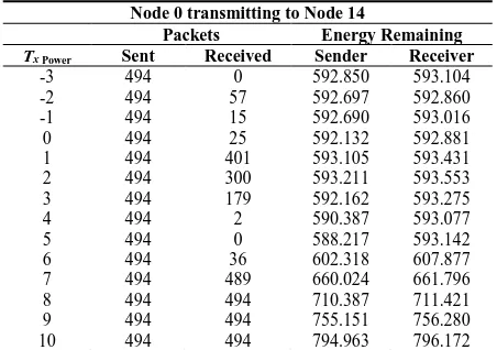
Scenario 2a consisted of 18 nodes in a horizontal grid formation of 6x3 nodes which is depicted in Figure 1. The nodes are placed 100 m apart. Node 0 is transmitting UDP packets to Node 14 and Node 3 is transmitting packets to Node 17. The timing of the transmissions has been synchronised, i.e. both Node 0 and Node 3 are scheduled to transmit to their respective destinations at the same time. Node 0 and Node 3 are transmitting UDP packets at approximately one packet per second.
In this scenario the interest was to determine how transmission power from multiple sources may cause interference and thus influence performance – a lower transmission power should cause less interference within the geographical area. The only varying parameter for the simulation runs in this scenario is the transmission power so that comparisons from Scenario 1a can be drawn.
Unlike Scenario 1, 14 simulation runs were conducted with transmission power ranging from -3 dB to +10 dB because it had been established from Scenario 1 that a transmission power less than -3 dB yields no received transmitted packets. Tables 12 and 13 present a summary of the results.
Node 0 transmitting to Node 14
Packets Energy Remaining
Tx Power Sent Received Sender Receiver
-3 494 0 592.850 593.104
-2 494 57 592.697 592.860
-1 494 15 592.690 593.016
0 494 25 592.132 592.881
1 494 401 593.105 593.431
2 494 300 593.211 593.553
3 494 179 592.162 593.275
4 494 2 590.387 593.077
5 494 0 588.217 593.142
6 494 36 602.318 607.877
7 494 489 660.024 661.796
8 494 494 710.387 711.421
9 494 494 755.151 756.280
10 494 494 794.963 796.172
Table 12. Summary of the results under Scenario 2a
(Node 0 to Node 14).
Node 3 transmitting to Node 17
Packets Energy Remaining
Tx Power Sent Received Sender Receiver
-3 494 0 592.778 593.766
-2 494 172 592.586 593.317
-1 494 0 592.775 593.408
0 494 28 592.171 593.347
1 494 430 593.048 593.422
2 494 269 593.010 593.552
3 494 149 592.314 593.277
4 494 99 590.208 593.052
5 494 0 590.516 593.127
6 494 33 602.300 607.864
7 494 491 659.923 661.790
8 494 494 710.398 711.398
9 494 494 755.180 756.254
10 494 494 794.986 796.143
Table 13. Summary of the results under Scenario 2a
(Node 3 to Node 17).
When transmission power was set to -3 dB no packets were received by neither destination, which is comparable with Scenario 1a, in addition to this the energy remaining at each node is also comparable. At -2 dB packets are successfully received by both destinations but performance is relatively poor with 88 % and 65 % packet loss, which is comparable with Scenario 1a, which experienced 79 % packet loss.
Network performance degraded even further when transmission power was set to -1 dB, in the case of node 17, no packets at all are received which is the same as
power to 0 resulted in an increase in performance but this was only a slight increase. When the transmission power was set to 1 dB performance increased significantly with node 14 receiving approximately 81 % of packets and node 17 receiving 87 % of packets.
Increasing the transmission power to 2 dB performance dropped, as the power increased (+3 dB, +4 dB and +5 dB) performance dropped in an almost linear fashion until no packets were received by either destination. Notably, energy consumption from -3 dB to +5 dB remains almost constant, this is depicted in Figure 12 and shown by the upper line.
Figure 12. Remaining Energy and Packets Sent/Received vs Transmission Power under
Scenario 2a.
Also depicted in Figure 12 is a slight increase in performance when increasing the transmission power from 5 dB to 6 dB. At transmission powers 7 dB to 10 dB performance is excellent, at 7 dB less than 1% of packets are not received whist from 8 dB to 10 dB all sent packets are received. Notably, as transmission power is increased power consumption is decreased in a linear fashion.
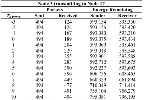
3.5 Scenario 2b
Scenario 2b is an adaption of Scenario 2a except rather than a constant mobility model the RWM was applied (Table 14). When applying the RWM, we did not want the nodes to wander outside of the boundaries of the original defined world (500 m x 200 m), therefore maximum x and y positional values for each node were set to 500 and 200 respectively. This kept the mobility of the node constrained within the original area defined. The RWM assigns points of the journey called waypoints, each node selects a speed between 0 m/s and 20 m/s and heads in a straight line from its current position to the waypoint. This process is repeated for each waypoint. There is the option for the node to pause at each waypoint but in this model the waypoint delay was set to 0, thus the nodes continually moved for the duration of the simulation.
Scenario 2b
Placement Model 6x3 Grid Distance between Nodes 100 Meters Mobility Model Random Waypoint
Maximum X Value 500
Maximum Y Value 200
Minimum Node Speed 0 m/s Maximum Node Speed 20 m/s
Waypoint Delay 0 s
Transport Protocol UDP
Data Rate 2048 B/s
Packet Size 2048 Bytes
Transmission Power -3 dB to +10 dB Data Capture Interval 5 s
Simulation Duration 500 s
Table 14. Setting under Scenario 2b.
When the RWM is applied there are no periods when packets are not received for all transmission powers simulated (-3 dB to 10 dB). As one might expect performance at -3 dB was poor and 81.38 % of packets were not received by node 14. Node 17 received slightly more packets, but the loss was still 74.90 %. As transmission increased there was an increase in performance for both destinations (-2 dB to 0 dB). Node 14 received slightly fewer packets when transmission power was changed from 0db to 1 dB, but this is only 1.49 % fewer packets and is negligible. When transmission power increased from 1 dB to 2 dB, Node 14 received more packets, however, this dropped again when transmission power was set to 3 dB. At 3 dB, Node 14 received 27 % fewer packet than when it was set to 2 dB. Node 14 then began to receive more and more packets as the transmission power was increased, however, it was not until transmission power was at 5 dB that more packets were received than when transmission power was set to 2 dB. At 6 dB, Node 14 saw a relatively sharp increase in performance, then from 7 dB to 10 dB perfomance increased but more gradually.
Figure 13. Remaining Energy and Packets Sent/Received vs Transmission Power under
The number of received packets for Node 17 showed no decline when transmission power was increased, as the transmission power increased so did the number of received packets.
Somewhat similar to all the other simulation runs is the amount of energy spent for the transmission power setting. At lower transmission power more energy is spent, as transmission power is increased (from 6 dB to 10 dB) less energy is spent. This is not attributed to failed transmissions and the need for retransmissions because the UDP protocol was used at the transport layer. UDP was specifically chosen as the transport layer protocol so that retransmissions would not influence the data (because retransmissions do not occur). Figure 13 depicts the results. Table 15 presents a summary of the number of sent packets from node 0 to node 14. Each row represents a simulation run using a different transmission power setting. Also shown in Table 15 is the total energy remaining at both the sender and the receiver when the simulations completed.
Node 0 transmitting to Node 14
Packets Energy Remaining
Tx Power Sent Received Sender Receiver
-3 494 92 593.157 593.337
-2 494 70 593.223 593.427
-1 494 130 592.965 593.305
0 494 201 592.992 593.419
1 494 198 592.676 593.453
2 494 261 592.559 593.393
3 494 190 592.395 593.491
4 494 255 592.345 593.679
5 494 285 592.548 593.723
6 494 427 607.081 608.503
7 494 436 660.285 661.885
8 494 451 709.893 711.417
9 494 470 754.832 756.307
10 494 478 795.164 796.192
Table 15. Summary of the results under Scenario 2b.
Node 3 transmitting to Node 17
Packets Energy Remaining
Tx Power Sent Received Sender Receiver
-3 494 124 593.154 593.350
-2 494 124 593.156 593.420
-1 494 167 593.040 593.310
0 494 189 593.075 593.434
1 494 204 593.069 593.461
2 494 229 593.018 593.548
3 494 255 592.901 593.588
4 494 283 592.712 593.675
5 494 390 592.237 593.693
6 494 396 606.756 608.463
7 494 449 660.329 661.894
8 494 477 710.049 711.414
9 494 491 755.104 756.279
10 494 494 795.081 796.195
Table 16. Summary of the results under Scenario 2b.
Table 16 presents a summary of sent packets from node 3 to node 17, like the previous table each row represents a simulation run using a different transmission power setting.
3.6 Scenario 2c
The final variation of Scenario 2 was to implement dynamic transmission power (i.e. Scenario 2c). In Scenario 2a and 2b the simulations ran for 500 seconds on a fixed transmission power, thus with 14 transmission power settings, 14 simulations were run each for 500 seconds. In this scenario the interest was to determine how energy depletion and performance would be impacted if transmission power was changing whist the simulation was running or ‘on the fly’. Therefore, Scenario 1c consisted of a single simulation with varying transmission power. The transmission power was increased every 24 s and begins at -10 dB incrementing to +10 dB. Table 17 reminds the reader of the scenario settings with the addition information regarding the duration of the increase time of transmission power.
Scenario 1c
Placement Model 6x3 Grid
Distance between Nodes 100 Meters
Mobility Model Constant
Transport Protocol UDP
Data Rate 2048 B/s
Packet Size 2048 Bytes
Transmission Power -10 dB to +10 dB Transmission Power Increment 24 seconds Data Capture Interval 5 seconds Simulation Duration 504 seconds
Table 17. Setting under Scenario 2c.
Table 18 presents a summary of the data every 24 seconds and Figure 14 shows the number of packets sent and received with the energy spent at the sender and the receiver for each transmission power setting for the communication between node 0 (sender) and node 14 (receiver). Table 19 and Figure 15 show the same summary information for communication between node 3 (sender) and node 17 (receiver).
Node 0 & Node 14
Packets Energy Spent
Tx Power Sent Received Sender Receiver
-10 23 0 19.657 19.658
-9 24 0 19.656 19.656
-8 24 0 19.657 19.656
-7 24 0 19.656 19.657
-6 24 0 19.656 19.656
-5 24 0 19.657 19.658
-4 24 0 19.695 19.694
-3 24 0 19.737 19.725
-2 24 4 19.779 19.764
-1 24 0 19.756 19.740
0 24 0 19.788 19.744
1 24 24 19.743 19.727
3 24 0 19.848 19.733
4 24 16 19.780 19.697
5 24 1 19.972 19.721
6 24 0 20.058 19.722
7 24 24 19.774 19.687
8 24 24 19.779 19.711
9 24 24 19.791 19.702
10 24 24 19.846 19.729
Table 18. Results under Scenario 2c.
Figure 14. Remaining Energy vs Transmission Power under Scenario 2c for Nodes 0 and Node 14.
Whilst transmission power was between -10 dB and -3 dB no packets were received by either destination (tables 18 and 19 and figures 14 and 15). Then at -2 dB some packets were received but 83 % approx. were lost, this is true for both destinations. At 0 dB no packets were received which was also true of both destinations. At 1 dB the number of received packet for both destinations significantly improves and transmissions are heard by the destinations, node 14 receives 100% of sent packets and node 17 receives 83% of packets. At 2 dB the number of received packets decreases for both destinations, node 14 receives 54.2 % and node 17 receives 45.8 %. At 3 dB there is a contrast between the number of packets received at each destination with Node 14 receiving no packets and Node 17 receiving 79.2 %. Then at 4 dB the reverse happens, Node 14 receives 66.6% and Node 17 receives 41.6 %. At 5 dB and 6 dB no packets are received for either destination (except Node 14 does receive 1 packet at 5 dB). Node 14 receives all packets that have been sent when transmission power is set between 7 dB and 10 dB. Node 17 does not receive any packets at 7 dB and around 20.8 % at 8 db. At 9 dB and 10 dB all packets are received at Node 17.
Node 3 & Node 17
Packets Energy Spent
Tx Power Sent Received Sender Receiver
-10 23 0 19.658 19.657
-9 24 0 19.656 19.657
-8 24 0 19.656 19.656
-7 24 0 19.657 19.656
-6 24 0 19.657 19.657
-5 24 0 19.657 19.657
-4 24 0 19.694 19.660
-3 24 0 19.734 19.684
-2 24 4 19.783 19.724
-1 24 0 19.757 19.724
0 24 0 19.791 19.715
1 24 22 19.745 19.727
2 24 11 19.708 19.701
3 24 19 19.777 19.736
4 24 10 19.712 19.696
5 24 0 19.721 19.720
6 24 0 19.719 19.721
7 24 0 19.680 19.679
8 24 5 19.717 19.708
9 24 24 19.794 19.700
10 24 24 19.839 19.734
Table 19. Results under Scenario 2c (Node 3 and Node 17).
Figure 15. Remaining Energy vs Transmission Power under Scenario 2c for Nodes 3 and Node 17.
4. Discussion
The original hypothesis was simple; reduce transmission power to the maximal optimal (the maximum transmission power required for successful stable communication) and produce a greener energy efficient network that can operate over a longer lifetime. Calculations show that with nodes spaced around 100 m apart the best transmission power would be -2 dB which gave a maximum optimal of 108 meters, a maximum of 110 meters and a mean of 107 meters (Table 20).
Distance
Tx Power Max
Optimal
Max Min
-20 14 14 12
-19 16 16 14
-18 18 18 16
-17 20 20 18
-16 22 22 20
-15 25 25 23
-14 26 28 25
-13 32 32 30
-12 35 35 33
-11 40 40 38
-10 44 44 42
-9 48 50 47
-8 52 55 52
-7 60 64 59
-6 66 71 66
-4 83 91 85
-3 95 99 96
-2 108 110 107
-1 122 124 121
0 133 138 134
1 148 167 151
2 167 182 168
3 185 200 191
4 210 223 215
5 232 247 241
6 260 283 270
7 295 310 304
8 339 347 342
9 367 400 382
10 410 460 430
11 461 506 481
12 525 564 539
13 585 623 605
14 657 729 678
15 736 796 763
16 829 930 864
17 908 1020 967
18 1025 1161 1084
19 1148 1280 1215
20 1286 1417 1355
Table 20. Transmission Power vs Distance.
However, from the analysis of the data produced by the simulations it is evident that although nodes are in communication range at -2 dB performance is somewhat poor. Table 21 presents an overview of the performance for each of the simulation runs at -2 dB.
Packets Energy Remaining
Scenario Sent Received Sender Receiver
1a 494 103 594.592 594.592
1b 494 351 594.592 594.592
1c 24 4 594.590 594.590
2a (0-14) 494 57 592.697 592.860 2a (3-17) 494 172 592.586 593.317 2b (0-14) 494 70 593.223 593.427 2b (3-17) 494 124 593.156 593.420
2c (0-14) 24 4 19.779 19.764
2c (3-17) 24 4 19.783 19.724
Table 21. Packets and Remaining Energy at -2 dB.
At -3 dB results were as expected, in most cases no packets were received with the exception for Scenarios 1b and 2b. According to the transmission range vs distance table a transmission power set to -3 dB could achieve at best 99 meters, with a maximal optimal at 95 meters and a mean of 96 meters. Some successful communication at -3 dB for Scenarios 1b and 2b is not so unexpected though because the random waypoint mobility model had been applied. Thus, the nodes begin at 100 meters apart but would have moved within the 95 - 99 m limits and at those periods successful communication could occur.
The most reliable communication was at much higher transmission levels, see Table 22, which summaries the
lowest transmission power for the highest number of received packets.
Packets Energy Remaining
Scenario Tx Power Sent Received Sender Receiver
1a 8dB 494 493 710.640 711.660 1b 6dB 494 351 608.175 609.013
1c 8dB 24 24 19.757 19.687
2a (0-14) 8dB 494 494 710.387 711.421 2a (3-17) 8dB 494 494 710.398 711.398 2b (0-14) 10dB 494 478 795.164 796.192 2b (3-17) 10dB 494 494 795.081 796.195 2c (0-14) 7dB 24 24 19.774 19.687 2c (3-17) 9dB 24 24 19.794 19.700
Table 22. Highest Number of Packets Received and Lowest Transmission Power.
The nature of the experiment involved communication within a MANET rather than mobile nodes in communication with an access point. This meant the routing of packets through intermediate nodes along a path to a destination occurs. One could assume that increasing the transmission power increased the power of the signal (thus the distance that signal could propagate), and as such, required fewer intermediate nodes for packets to traverse to the destination. This assumption would be correct.
However, in Scenario 1 the world consisted of a 200 m x 200 m geographical area. Therefore, for node 0 to be in direct communication range of node 8 (each at opposite ends of the world) we can calculate their distance using the Pythagorean theorem.
√
(𝑥2− 𝑥1)2+ (𝑦2− 𝑦1)2This yields a distance between the source node and destination node of ≈ 282.84 meters. According to the transmission vs. distance table, a transmission power of 7 dB could easily accommodates this distance (i.e. a maximum optimal of 295, with a maximum of 310 and a mean of 304). However, Scenarios 1a and 1c required a transmission distance of at least 8 dB for optimal performance. Scenario 1b only required 6 dB but as stated earlier the nodes would have moved within closer proximity.
In Scenario 2 the world consisted of a 500 m x 200 m geographical area, however, node 0 transmitted to node 14 and node 3 transmitted to node 17, which gave the distance between the two communicating parties as ≈ 282.84 m, so would have been easily in range of their respective destinations at 7 dB. However, for the most optimal packet delivery ratio at least 8 dB was required for Scenario 2a.
These results show that ideally nodes should be in direct communication range for optimal performance with a transmission power setting higher than the maximum optimal. The reason for this is because in a MANET, packets are routed through intermediate nodes and as a result, routing algorithms generate their own routing traffic to discover and maintain routes, in addition to this routing information is propagated throughout the network. The higher than required transmission power setting helps with this noisy communication medium.
The main goal of this research was to show the most optimal transmission power to conserve energy in a MANET to make that network ‘greener’ and to increase the lifetime of that network.
Thus, we are interested in the energy remaining at the end of each simulation run. Table 23 presents a table that shows the transmission power setting that conserves the most energy (energy began at 1000).
Packets Energy Remaining
Scenario TxPower Sent Received Sender Receiver
1a 10dB 494 493 795.185 796.342
1b 10dB 494 493 795.159 796.331
1c 10dB 24 24 19.811 19.698
2a (0-14) 10dB 494 494 794.963 796.172
2a (3-17) 10dB 494 494 794.986 796.143
2b (0-14) 10dB 494 478 795.164 796.192
2b (3-17) 10dB 494 494 795.081 796.195
2c (0-14) 10dB 24 24 19.846 19.729
2c (3-17) 10dB 24 24 19.839 19.734
Table 23. Packets and Remaining Energy at -2 dB.
Table 23 shows that increasing the transmission power conserves energy. The likely reason for this is because traffic propagates over greater distances so there is less call on the route discovery process, thus conserving energy by propagating less routing information.
5. Conclusion
In this research, it has been shown that there is an optimal transmission power setting that results in both greater network performance regarding packet delivery ratio and less energy consumption. Therefore, the network performs optimally whilst conserving energy, which results in a greener more energy efficient network. The research consisted of an analysis of 72 simulations (both with static transmission power and dynamically changing transmission power) and from this analysis we conclude that all simulations resulted in a consistent message.
Future research could involve moving away from setting uniformly transmission power output to determine if an optimal transmission power setting can be obtained my making better use of intermediate nodes. This would account for nodes that do not need to transmit signals as far as other nodes. It would also be interesting to research the power consumptions across different protocols, for
example, does the Temporally Ordered Routing Algorithm (TORA) routing protocol use as much energy as the Destination-Sequenced Distance Vector (DSDV) routing protocol in establishing the routes? This research builds upon many others’ research, for example, [11-12, 14, 17-18] but with the added feature of being able to determine an optimal transmitting power in a MANET.
Acknowledgements
We thank all staff of the School of Computer Science, University of Manchester, the Department of Computing Science and Mathematics, University of Stirling, the Institut National Des Sciences Appliquees and the Department of Mathematics & Computer Science, Liverpool Hope University.
References
[1] J.B. Hughes, P. Lazaridis, I. Glover and A. Ball, "A survey of link quality properties related to transmission power control protocols in wireless sensor networks," 23rd International Conference on Automation and Computing (ICAC), Huddersfield, 1-5, 2017.
[2] J.B. Hughes, P. Lazaridis, I. Glover and A. Ball, "Opportunities for transmission power control protocols in wireless sensor networks," 23rd International Conference on Automation and Computing (ICAC), Huddersfield, 1-5, 2017.
[3] W.R. Heinzelman, A. Chandrakasan and H. Balakrishnan, "Energy-efficent communication protocol for wireless microsensor networks," in Proc. Hawaii Int. Conf. System Sciences, Maui, Hawaii, 2000.
[4] W. He, S. Nabar, and R. Poovendran. "An energy framework for the network simulator 3 (ns-3)." In Proc. 4th International Conference on Simulation Tools and Techniques (ICST), 222-230, 2011.
[5] D. Halperin, B. Greenstein, A. Sheth, and D. Wetherall. Demystifying 802.11n power consumption. In Proc. International Conference on Power Aware Computing and Systems (HotPower'10), Berkeley, CA, USA, 2010. [6] A. Zarei Ghanavati and D. Lee, "Optimizing the Bit
Transmission Power for Link Layer Energy Efficiency under Imperfect CSI," in IEEE Transactions on Wireless Communications, 99, 1-1.
[7] R. Kotian, G. Exarchakos and A. Liotta, "Reliable low-power wireless networks over unstable transmission power," IEEE 14th International Conference on Networking, Sensing and Control (ICNSC), Calabria, 801-806, 2017. [8] P.P. Priyesh and S.K. Bharti, "Dynamic transmission power
control in wireless sensor networks using P-I-D feedback control technique," 9th International Conference on Communication Systems and Networks (COMSNETS), Bengaluru, 306-313, 2017.
[9] U. Ghosh and R. Datta, "A Secure Addressing Scheme for Large-Scale Managed MANETs," in IEEE Transactions on Network and Service Management, 12(3), 483-495, Sept. 2015.
Systems Informatics, Modelling and Simulation (SIMS), Riga, 153-158, 2016.
[11] Tiwari and I. Kaur, "Performance evaluation of energy efficient for MANET using AODV routing protocol," 3rd International Conference on Computational Intelligence & Communication Technology (CICT), Ghaziabad, 1-5, 2017. [12] M. Ilango and A.V.S. Kumar, "Deterministic multicast
link-based energy optimized routing in MANET," 2nd International Conference on Electrical, Computer and Communication Technologies (ICECCT), Coimbatore, Tamil Nadu, India, 1-10, 2017.
[13] W. Feng, H. Luo, B. Sun and C. Gui, "Performance analysis of sliding window network coding for energy efficient in MANETs," 7th IEEE International Conference on Electronics Information and Emergency Communication (ICEIEC), Macau, 219-222, 2017.
[14] S. Prajapati, N. Patel and R. Patel, "Optimizing Performance of OLSR Protocol Using Energy Based MPR Selection in MANET," 5th International Conference on Communication Systems and Network Technologies, Gwalior, 268-272, 2015.
[15] W. Feng, H. Luo, B. Sun and C. Gui, "Performance analysis of sliding window network coding for energy efficient in MANETs," 7th IEEE International Conference on Electronics Information and Emergency Communication (ICEIEC), Macau, 2017, 219-222.
[16] H.T. Friis, "A Note on a Simple Transmission Formula," in Proc. of IRE, 34(5), 254-256, May 1946.
[17] M. Lanati, D. Curone, E.L. Secco, G. Magenes, P. Gamba, An autonomous long range monitoring system for emergency operators, International Journal of Wireless & Mobile Networks, 3(1), 10-23, 2011.