www.nat-hazards-earth-syst-sci.net/10/2407/2010/ doi:10.5194/nhess-10-2407-2010
© Author(s) 2010. CC Attribution 3.0 License.
and Earth
System Sciences
Tsunami waves generated by submarine landslides of variable
volume: analytical solutions for a basin of variable depth
I. Didenkulova1,2, I. Nikolkina2,3, E. Pelinovsky2,3, and N. Zahibo3 1Laboratory of Wave Engineering, Institute of Cybernetics, Tallinn, Estonia
2Department of Nonlinear Geophysical Processes, Institute of Applied Physics, Nizhny Novgorod, Russia
3Laboratory of Research in Geosciences and Energy, University of the French West Indies and Guiana, Guadeloupe, France Received: 25 May 2010 – Revised: 18 October 2010 – Accepted: 21 October 2010 – Published: 30 November 2010
Abstract. Tsunami wave generation by submarine landslides of a variable volume in a basin of variable depth is studied within the shallow-water theory. The problem of landslide induced tsunami wave generation and propagation is studied analytically for two specific convex bottom profiles (h∼x4/3 and h∼x4). In these cases the basic equations can be reduced to the constant-coefficient wave equation with the forcing determined by the landslide motion. For certain conditions on the landslide characteristics (speed and volume per unit cross-section) the wave field can be described explicitly. It is represented by one forced wave propagating with the speed of the landslide and following its offshore direction, and two free waves propagating in opposite directions with the wave celerity. For the case of a near-resonant motion of the landslide along the power bottom profileh∼xγ the dynamics of the waves propagating offshore is studied using the asymptotic approach. If the landslide is moving in the fully resonant regime the explicit formula for the amplitude of the wave can be derived. It is demonstrated that generally tsunami wave amplitude varies non-monotonically with distance.
1 Introduction
The landslide motion is now recognized as an important source of tsunami wave generation, since it is the second most frequent tsunami source after earthquakes responsible for about 10% of all tsunami waves (Gusiakov, 2009).
Correspondence to: I. Nikolkina ([email protected])
At least, two special workshops specialized on this problem should be mentioned (Keating et al., 2000; Yalciner et al., 2003).
For example, an underwater landslide on 17 July 1998 caused the destructive Papua New Guinea tsunami, when the 15-m wave at the coast devastated three villages and took more than 2200 lives (McSaveney et al., 2000; Synolakis et al., 2002). On 17 August 1999 a shore slump in the Izmit Bay (Turkey) generated a 2.5 m high tsunami (Altinok et al., 2001). The problem of tsunami generation by landslides has also been actively discussed in the Atlantic and Caribbean. In particular, three tsunamis in the Lesser Antilles were generated by avalanche flows from the Montserrat volcano in 1997, 2003 and 2006 (O’Loughlin and Lander, 2003; Pelinovsky et al., 2004; Zahibo, 2006). Deplus et al. (2001) reported large-scale debris avalanche deposits around the Lesser Antilles. Particularly, a large area covered by mega blocks up to 2.8 km long and 260 m high is located off Dominica. Large coastal landslides and associated tsunami hazard in the Caribbean are described in (Teeuw et al., 2009). According to their study possible tsunami waves in the vicinity of Dominica can reach 3–10 m due to probable collapse of coastal blocks. Thus, the problem of tsunami generation by landslides is of current scientific interest.
of the erosion processes in avalanches, so that the deposited mass in the runout zone can be much larger than the initial mass in the starting zone. This effect of variable volume of the landslide has never been analyzed in the problem of tsunami wave generation and the given study is focused on this problem.
The number of analytical methods for analysis of tsunami wave generation by submarine landslides is limited even for the cases when the landslide is moving with a constant speed and conserves its volume. 1-D wave field around landslide moving with a constant speed in a basin of constant depth is computed in (Pelinovsky, 1996, 2003; Tinti and Bortolucci, 2000; Tinti et al., 2001; Okal and Synolakis, 2003). The 2-D and 3-D motion of a constant-speed landslide is studied analytically for shallow-water approximation in the framework of the potential theory in (Novikova and Ostrovsky, 1978; Pelinovsky and Poplavsky, 1997; Ward, 2001). The landslide tsunami generation along a sloping beach in 1-D and 2-D cases is discussed in (Liu et al., 2003; Sammarco and Renzi, 2008), in the last case the landslide also induces edge waves propagating along a plane beach.
An interesting analytical example of tsunami wave generation in the shallow water basin of variable depth is given in (Tinti et al., 2001). It was shown that in the case of bottom profileh∼x4/3 (h is the water depth and x is coordinate directed offshore) the wave equation with an external force can be simplified and the same methods as for a constant depth basin can be applied. It was found later in (Didenkulova et al., 2009) that this bottom profile can be interpreted as a “non-reflecting” one. Waves propagating along this profile in the opposite directions do not interact between each other and are able to transfer the wave energy over large distances. At the same time there is another quartic bottom profile, h∼x4, which has the same “non-reflecting” nature (Didenkulova and Pelinovsky, 2010) and the analytical solution of the tsunami wave generation by landslides along this profile is studied below in detail. In fact, the number of “non-reflecting” profiles in 1-D geometry exceeds two, but other bottom configurations lead to the wave dispersion even in the shallow-water approximation (Grimshaw et al., 2010).
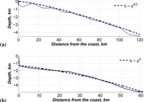
At the same time real bathymetries in the coastal zone can be well approximated by these two “non-reflecting” profiles. For example, Fig. 1 demonstrates the applicability of “non-reflecting” approximation to bottom profiles near Guadeloupe, Caribbean Sea (Gusiakov, 2002).
Here we present an analytical study of tsunami wave generation by landslides of a variable volume moving with a variable speed in 1-D case. The mathematical model that is linear shallow-water theory is briefly described in Sect. 2. The process of tsunami wave generation along a special beach profileh∼x4/3is studied in Sect. 3. Here, in contrast to Tinti et al. (2001) the landslide is assumed to have a volume variable per unit cross-section and velocity variable during its motion. The runup of generated tsunami waves
(a)
(b)
Fig. 1. Bottom profiles near Guadeloupe, Caribbean Sea (solid line)
and their “non-reflecting” approximations (dashed line); (a) Marie-Galante and (b) La Desirade.
on this beach is also analyzed. The generation of tsunami waves along a quartic bottom profileh∼x4is discussed in Sect. 4 and the new analytical solution for landslide induced tsunamis is studied in detail. The case of the resonant generation of tsunami waves by landslides above slowly varying “power” bottom profile and its propagation offshore is considered in Sect. 5. Using the asymptotic approach, the wave field is expressed analytically in the integral form and discussed for various scenarios, when the volume of the landside increases, decreases or stays constant with time. It is shown that generally the wave amplitude varies with offshore distance non-monotonically due to competing effects of the resonant growth and the wave attenuation with a depth. The main results are summarized in Sect. 6.
2 Basic model
The governing equations of 1-D linear shallow-water theory for tsunami wave generation by underwater landslides are (Pelinovsky, 1996; Tinti et al., 2001; Liu et al., 2003):
∂η ∂t +
∂
∂x[h(x)u]=W (x,t )= ∂zb
∂t , (1)
∂u ∂t +g
∂η
∂x=0, (2)
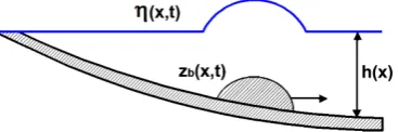
whereη(x,t )is the water displacement,u(x,t )is the depth-averaged flow velocity,gis the gravity acceleration,W (x,t ) is the vertical velocity of the moving bottom boundary zb(x,t ); see Fig. 2.
Initial conditions for the shallow-water system (1)–(2) are applied to both the water displacement η(x,t ) and depth-averaged flow velocityu(x,t ). If at the initial moment the ocean rests, they are
Fig. 2. The geometry of the problem: the water displacement
η(x,t )is generated by the landslide with the shapezb(x,t )above
the variable bottom profileh(x).
These initial conditions (3) are used in (Tinti et al., 2001; Liu et al., 2003). Meanwhile, if the vertical velocity of the landslide, W, is nonzero at the initial moment, that is a typical approximation in this kind of a problem. It follows from Eq. (1) that the vertical velocity of the fluid (∂η/∂t) is also nonzero. In fact, flow distribution around the body with nonzero velocity is more complicated and should be found by solving the full system of hydrodynamic equations. So the ratio between vertical and horizontal components of velocity is not evident in the shallow-water approximation. For example, Pelinovsky (1996, 2003) assumed that the vertical velocity (∂η/∂t) is zero at the initial moment.
Here we consider the situation of the landslide movement triggered by the earthquake that in the initial moment the landslide body lifts up and then slides down. Of course, the shallow water theory does not give a correct representation of the early fluid motion from rest. In the literature this paradox has been specially studied for the piston-model of tsunami wave motion. As it has been shown by (Kajiura, 1963) and then reproduced by (Kervella et al., 2007), if the size of the landslide is four times larger than the water depth, in shallow water theory and in full hydrodynamic model the shape of the free water surface (for the most part of the initial disturbance) coincide. The study was based on the rectangular initial disturbance and the only discrepancy between these two models was found at the sharp ends of the rectangular pulse, and this discrepancy can be smoothed by filtering. This explains why the shallow water theory is widely used for the description of the initial stage of the landslide motion. In all our calculations below we consider only smooth initial disturbances that justify the applicability of the shallow water model.
In this case the appropriate initial conditions should be derived from the assumption that the landslide velocity is zero at the initial moment as it is rigorously applied to the problem of wave generation by a moving bottom (“piston” model). Using the analogy with the piston model of tsunami generation let us consider the following approximation of the moving bottom:
zb(x,t )=Y (t )Zb(x,t ), (4) where Zb(x,t ) is a “smooth” function, that describes the landslide motion (for example, constant-speed motion), and
Y (t )is almost the step function, which reflects the transition process when the landslide suddenly starts its motion. After integrating Eqs. (1) and (2) over an infinitesimal time interval the new initial conditions for the system (1)–(2) with an external forcingW=∂Zb/∂tcan be obtained
η(x,0)=Zb(x,0), u(x,0)=0. (5) These effective initial conditions (5) are well known for the piston shift of the bottom during the earthquake. Mathematically, nonzero initial conditions appear in the hyperbolic equations with an external forcing if the Cauchy problem is posed in the class of generalized functions (in our case it is a step function, which reflects sudden motion of the landslide) (Courant and Hilbert, 1989).
Equations (1) and (2) of the shallow-water system can be reduced to the wave equation for the water displacement (Zb is replaced byzb)
∂2η ∂t2−
∂ ∂x
c2(x)∂η ∂x
=∂
2zb
∂t2 , c= p
gh(x), (6) which satisfies the following initial conditions
η(x,0)=zb(x,0), ∂η ∂t(x,0)=
∂zb
∂t (x,0). (7) Alternatively, the wave equation for the flow velocity
∂2u
∂t2− ∂2
∂x2 h
c2(x)ui= −g∂ 2z
b
∂t ∂x, (8)
satisfies the initial conditions u(x,0)=0, ∂u
∂t(x,0)= −g ∂zb
∂x(x,0). (9) We would like to stress that both initial conditions (7) and (9) are derived from a more general assumption (5) and are equivalent.
Each form of the wave equation: Eq. (6) or Eq. (8) has its advantages in different problems and for different bottom configurations. Analytical solutions of both Eqs. (6) and (8) are discussed in Sects. 3 and 4, respectively. It is also important to mention here that the landslide described by the function zb(x,t )can have a variable volume and move with a variable speed. Different scenarios of the landslide body change, when its volume increases, decreases or stays constant are studied in Sect. 5.
3 Tsunami generation by the landslide motion along the bottom profileh∼x4/3
Let us consider here the bottom profile described by
h(x)=px4/3, (10)
x=0 corresponds to the shoreline. As it has been shown in Didenkulova et al. (2009), long waves propagating along a bottom profile (10) do not interact between each other and conserve their shape, while their amplitude satisfies the Green’s law (h−1/4). In comparison with the water displacement, the velocity field has a more complicated form: the shape of the wave of velocity changes in time and its amplitude does not satisfy the Green’s law. Formally, the water displacement disturbance can be considered as a traveling wave transferring the potential wave energy over large distances. The detailed analysis of the long wave dynamics along the bottom profile (10) including the process of the wave runup on the coast is given in (Didenkulova et al., 2009) for various initial disturbances.
Mathematically, this “non-reflecting” behavior is related to the possibility of reduction of the variable-coefficient wave equation to the constant-coefficient wave equation. In the case of the bottom profile (10) this reduction was first applied to the problem of tsunami generation by a moving landslide by (Tinti et al., 2001). The transformation (x0 and h0 represent the coordinate and the depth of the initial landslide location, respectively)
η(x,t )=A(x)H (τ (x),t ), τ=
x Z
x0 dx0 c(x0),
A(x)=A0 h
0 h(x)
1/4
, (11)
reduces Eq. (6) to the constant-coefficient wave equation with an external forcing
∂2H ∂t2 −
∂2H ∂τ2 =
∂2 ∂t2 zb(τ,t ) A(τ ) . (12)
The solution of Eq. (12) satisfying the initial conditions (7) can be expressed in the Duhamel integral form (Courant and Hilbert, 1989):
H (τ,t )=1
2
zb(τ−t ) A(τ−t )+
zb(τ+t ) A(τ+t ) +1 2 τ+t Z τ−t 1 A(σ ) ∂zb ∂t (σ,0)dσ +1 2 t Z 0 dρ τ+(t−ρ) Z τ−(t−ρ) 1 A(ς )
∂2zb
∂ρ2(ς,ρ)dς. (13) Similar solution with some modifications due to other initial conditions was used in (Tinti et al., 2001) for tsunami waves generated by the landslide moving with a constant speed. Obtained results were compared with those for a flat bottom and the difference was relatively small.
Equation (13) can be presented in the explicit form for the following landslide motion:
zb(τ,t )=A(τ )Z (τ−Fr·t ), (14)
where Fr is the constant Froude number, which determines the variable speed of the landslide
V (x)=dx
dt =c(x)·Fr. (15) The landslide body according to Eq. (14) has the variable volume (mass) per unit cross-section
M(t )= Z
zb(x,t )dx= Z
c(τ )A(τ )Z(τ−Fr·t )dτ. (16) IfZ(τ )is defined as a stepwise function, whereτ0andT are arbitrary constants, which define the location and the length of the landslide,
Z(τ )=
0, τ < τ0, 1, τ0< τ < τ0+T 0, τ > τ0+T ,
, (17)
Eq. (16) simplifies to M(t )=M0
1+ Fr
τ0+T /2 t
. (18)
Thus, the landslide moves with acceleration proportional to t (∼x1/3 or ∼h1/4), its height decreases with time as t−1 (∼x−1/3), but the volume grows with time and with distance (∼x1/3). The length of the landslide also increases (∼x2/3). Therefore not all the points of the landslide move at the same speed. The growth of the landslide volume can be connected to the bottom sediment friction; so that the landslide “absorbs” the surrounding materials and makes bottom particles “cling” to it. This physical process is well known for avalanches and described in (Pudasaini and Hutter, 2007). It is important to emphasize that variations of the landslide parameters (its acceleration, height and volume) with the depth are relatively slow (∼h1/4) and therefore, the process of the wave generation by the landslides along the bottom profile (10) can be considered as qualitatively the same as in the basin of constant depth.
Equation (13) for the special landslide shape (14) transforms into
H (τ,t )= Fr
2
Fr2−1Z (τ
−Fr·t )− 1
2(Fr−1)Z(τ−t )
+ 1
2(Fr+1)Z(τ+t ). (19)
Solutions, similar to Eq. (19) are known for tsunami waves induced by landslides moving with a constant speed in a basin of constant depth (Pelinovsky, 1996, 2003; Tinti et al., 2001). In physical variables the solution (19) has the following form
η(x,t )= Fr
2
Fr2−1A(x)Z Z
dx c(x)−Fr·t
− A(x)
2(Fr−1)Z
Z dx
c(x)−t
+ A(x)
2(Fr+1)Z
Z dx
c(x)+t
and represents three waves. The first one is the forced wave, which is located above the landslide and moves with the variable velocity (15); its length increases with a distance and its amplitude is proportional to the landslide height and decreases with a distance. The forced wave is positive (wave of elevation) in super-critical regime (Fr>1) and negative (wave of depression) in sub-critical regime (Fr<1). The second wave is a free wave, which moves with a variable velocityc(x)behind the landslide in the super-critical regime (Fr>1) and in front of it in sub-critical regime (Fr<1). Its amplitude decreases and its length increases in time. The third (free) wave moves shoreward with an increase in its amplitude and decrease in length. The relation between amplitudes of these waves for different values of the Froude number at the moment of wave generation is illustrated in Fig. 3.
Here the amplification factor is the ratio H /Z marked in dashed blue for the first term, dash-dotted red – for the second and solid black – for the third. The resonance between waves and the landslide (Fr≈1) dramatically increases amplitudes of waves moving offshore (in the direction of the landslide). At the same time these waves do not split in space in the vicinity of the resonance and, therefore, the resulting amplitude also stays bounded for a long time. For exact resonance (Fr = 1) Eq. (20) transforms into
η(x,t )= −A(x)t
2 ∂Z
∂τ[τ (x)−t]+ 3A(x)
4 Z[τ (x)−t]
+A(x)
4 Z[τ (x)+t]. (21)
The forced wave propagating offshore has a sign-variable shape. Taking into account that in the vicinity of the resonanceτ (x)≈t, the resonant wave can be written as ηres(x,t )= −
A(x)τ (x) 2
∂Z
∂τ[τ (x)−t]. (22)
As a result, wave amplitude grows with the distance and tends to the asymptotic value
A∞=3x0
c0
A0max(∂Z/∂τ ). (23)
In contrast to the basin of a constant depth, where the resonance leads to the infinite growth of the wave amplitude, the resonant effect in the basin of a variable depth can be bounded. Detailed study of these effects is given in Sect. 5.
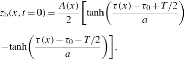
The wave dynamics along the beach profile (10) with the same parameterpas for the coast of Marie-Galante (Fig. 1a) is calculated below for the initial landslide shape (Fig. 4), described by
zb(x,t=0)=A(x)
2
tanh
τ (x)−τ 0+T /2 a
−tanh
τ (x)−τ0−T /2 a
, (24)
0 0.5 1 1.5 2
−8 −6 −4 −2 0 2 4 6 8
Amplification factor
Froude number
Fig. 3. Amplification factor for generated tsunami waves along
the bottom profileh∼x4/3plotted against the Froude number: the forced wave (dashed blue line) and free waves propagating offshore (dash-dotted red line) and onshore (solid black line).
6 6.5 7 7.5 8 8.5 9
0 0.2 0.4 0.6 0.8 1
x (km)
Initial landslide displacement (m)
Fig. 4. Initial landslide shape (24) along the bottom profileh∼ x4/3.
whereT =30 s and τ0=11 min, providing the location of 2 km long and 1 m high landslide at the distance 7.5 km offshore at the water depth 100 m. Parameter a=0.3T is chosen to provide smoothing of the landslide shape. Similar parameters of the landslide were used in the paper by Tinti et al. (2001), and they are also in agreement with estimations of possible and real submarine landslides in the Lesser Antilles (Ten Brink et al., 2006; Teeuw et al., 2009).
Fig. 5. Wave dynamics along the bottom profile h∼x4/3 in subcritical (blue dashed line) and supercritical (black line) regimes.
(a)
10 12 14 16 18 20
0 0.5 1 1.5 2 2.5 3
Distance from shore, km
Maximum wave amplitude, m
Fr = 0.8 Fr = 1.2
A ~ h−1/4
(b)
0 1 2 3 4 5 6 7
0 0.2 0.4 0.6 0.8 1
Distance from shore, km
Maximum wave amplitude, m
Fr = 0.8 Fr = 1.2 A ~ h−1/4
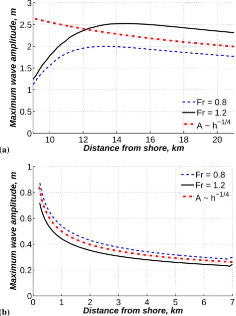
Fig. 6. Variations of the maximum amplitude of tsunami waves
during its propagation along the bottom profile h∼x4/3: for positive waves propagating offshore (a) and onshore (b).
of their amplitudes are presented in Fig. 6a. In the beginning for a short time amplitudes of individual waves propagating offshore are increased by the resonant effect up to the factor of 2.5 in the case of the supercritical regime (Fr = 1.2) but at the distance of about 2–3 wavelengths they start to be determined by the functionA(x)∼h(x)−1/4∼x−1/3, which reflects the Green’s law (Fig. 6a). The main difference between two studied regimes is that waves propagating offshore are higher and faster in the case of the supercritical regime even if the deviation from the critical value of the Froude number is the same.
The free wave of the third term in Eq. (19) moves onshore with a weak initial amplitude that grows when the wave approaches the coast (Fig. 7). The wave approaching the beach increases in its amplitude according to the Green’s law (Fig. 6b) and reduces in length. The wave amplitude is higher in the subcritical regime rather than in supercritical one. The shoaling effect becomes significant near the shore and gives wave amplification in several times (2–3 times).
0 100 200 300 400 500 600 −3
−2 −1 0 1 2
Distance from shore, m
Water displacement, m t = 8 min
0 100 200 300 400 500 600
−3 −2 −1 0 1 2
Distance from shore, m
Water displacement, m t = 10 min
Fig. 7. Tsunami wave runup on the beachh∼x4/3in subcritical (blue dashed line) and supercritical (black line) regimes.
described by Eq. (10) in comparison with a plane beach (Synolakis, 1987; Didenkulova et al., 2007, 2008), since the linear wave equation is solved. Estimates of the wave runup on the beach, described by Eq. (10), give unfeasibly high runup height (Didenkulova et al., 2009). That is why we match the non-reflecting beach (Eq. 10) with the beach of constant slope, for which the nonlinear problem of runup is solved, in the point, where the wave amplitude is small in comparison with the water depth. In our case it is the distanceX1∼500−600 m from the shore. The process of the wave runup on a plane beach is well-studied (Synolakis, 1987; Didenkulova et al., 2007, 2008) and the runup height can be determined (Didenkulova et al., 2008)
Rplane≈3.5ApX1/λ, (25) where A and λ are amplitude and wavelength of the approaching wave at the distance X1 from the shore respectively. Taking into account wave parameters at the distanceX1∼500 m from the shore: amplitude A∼0.7 m and wavelength is λ∼200 m, the runup height can be estimated from Eq. (25) as 3.9 m. It follows from Eq. (20) that amplitude of incoming wave decreases with an increase in the Froude number. Hence, the runup height also decreases with an increase in the Froude number as
∼1/(Fr+1).
At the same time, since the water depth in the near shore is too small (a few meters) it is reasonable that the dissipation of wave energy in the near-bottom turbulent flow and the wave breaking lead to the decrease in the tsunami runup height. As it is shown in (Didenkulova et al., 2010) usually landslide generated tsunami waves break at the coast. Thus, the results presented here can be considered as the upper estimate for the possible tsunami runup heights.
4 Tsunami generation by the landslide motion along the quartic bottom profileh∼x4
Another bottom profile, which allows analytical solution for the problem of tsunami wave generation by landslides, is
h(x)=qx4, (26)
whereqis an arbitrary coefficient with the dimension m−3. As it has been recently shown in (Didenkulova and Pelinovsky, 2010), similarly to the wave dynamics along the bottom profile (10) discussed in Sect. 3, long waves of the flow velocity do not interact between each other along the quartic bottom profile, described by Eq. (1). These propagating waves of flow velocity do not change their shape in time and their amplitudes satisfy the Green’s law for velocity (h−3/4). In contrast to the case of the bottom profile, described by Eq. (10), the water displacement along the quartic bottom profile does not have a simple representation: the wave shape is not conserved and its amplitude does not satisfy the Green’s law. The detailed analysis of the wave dynamics in this case for various initial disturbances is given in (Didenkulova and Pelinovsky, 2010).
Similarly to the case discussed in Sect. 3, the simplified behavior along the quartic bottom profile is related to the possibility of reduction of the variable-coefficient wave equation to the constant-coefficient wave equation. The following transformation
u(x,t )=B (x)U (τ (x),t ),
τ= − Z dx
c(x), B (x)=bh
−3/4(x), (27)
whereb is an arbitrary constant with dimension m7/4s−1, reduces the wave equation for the flow velocity with an external forcing (8) to the inhomogeneous constant-coefficient wave equation
∂2U ∂t2 −
∂2U ∂τ2 = −
g B (τ )c(τ )
∂2zb(τ,t )
∂t ∂τ . (28) Initial conditions for Eq. (3) follow from Eqs. (9) for velocity flow that is identical to Eqs. (7) for water displacement U (τ,0)=0, ∂U
∂t (τ,0)= − g B(τ )c(τ )
∂zb
from the previous case of the beach (10), described in Sect. 3. It means that in the new variables the landslide moves to the left.
Similarly to the case described in Sect. 3, the solution of Eq. (3) satisfying the initial conditions (4) can be represented in the form of the Duhamel integral (Courant and Hilbert, 1989):
U (τ,t )= −1
2 τ+t Z
τ−t g B(σ )c(σ )
∂zb
∂σ(σ,0)dσ
−1
2 t Z
0 dρ
τ+(t−ρ) Z
τ−(t−ρ) g B(ς )c(ς )
∂2zb
∂ρ∂ς(ς,ρ)dς. (30) The new forcing function
P (τ,t )=
Z g
B(τ )c(τ )
∂zb(τ,t )
∂τ dτ, (31)
simplifies Eqs. (28) and (29) and transforms them to ∂2U
∂t2 − ∂2U
∂τ2 = −
∂2P (τ,t )
∂t ∂τ , (32)
U (τ,0)=0, ∂U
∂t (τ,0)= − ∂P
∂τ(τ,0). (33) If the new forcing function (31) of the landslide motion can be presented in the following way
P (τ,t )=P (τ+Fr·t ), (34) Eq. (30) transforms into a simple explicit solution for the velocity field
U (τ,t )= − Fr Fr2−1P (τ
+Fr·t )
+ 1
2(Fr−1)P (τ+t )+ 1
2(Fr+1)P (τ−t ), (35) which represents three waves of velocity, the first of which is the forced one propagating offshore (the first term in Eq. 35), and other two are free waves propagating offshore and onshore respectively. The amplitude of the forced wave propagating offshore in dimensionless variables varies linearly with time in the vicinity of the resonance (Fr = 1) U (τ,t )= −t
2
∂P (τ+t ) ∂τ −
1
4P (τ+t )+ 1
4P (τ−t ). (36) The water displacement can be found from Eq. (2)
∂η ∂τ= −bq
1/4τ∂U
∂t , (37)
using the condition of zero displacement at infinityx→ ∞
that corresponds toτ=0.
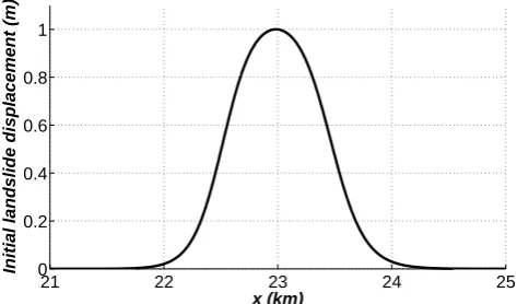
21 22 23 24 25
0 0.2 0.4 0.6 0.8 1
x (km)
Initial landslide displacement (m)
Fig. 8. Initial landslide shape (38) along the quartic bottom profile
h∼x4.
The long wave dynamics along the quartic bottom profile is discussed for the landslide shape (Fig. 8) given by
zb(x,t=0)= A0
2
tanh
τ (x)−τ0+T /2 a
−tanh
τ (x)−τ 0−T /2 a
, (38)
whereτ0 represents the travel time to the deep water. The landslide shape in Eq. (38) differs from the one discussed in Sect. 3 (Eq. 24) by the amplitude A. It is constant in Eq. (38), while in Eq. (24) it is a function of coordinateA(x), representing the Green’s law. Though the solution (Eq. 35) describing the long wave dynamics along the quartic profile is very similar to the one, discussed in Sect. 3, there are some differences, which should be mentioned. The depth of a quartic bottom profile is a rapid function of the distance far from the coast that leads to the fact that long waves cross the deep water in a fixed time. It is evident that the shallow-water approximation breaks down on large depths and the solution given by Eq. (35) does not work there.
Fig. 9. Wave dynamics along the quartic bottom profileh∼x4in subcritical (blue dashed line) and supercritical (black line) regimes.
24 26 28 30 32 34
0 1 2 3 4 5
Distance from shore, km
Maximum wave amplitude, m
Fr = 0.8 Fr = 1.2 A~h−1/4
Fig. 10. Variations of the maximum amplitude of tsunami waves
during its propagation along the quartic bottom profileh∼x4for positive waves propagating offshore.
The calculated long wave dynamics along the quartic bottom profile with the parameter q taken from the bathymetry near Desirade (Fig. 1b) for the landslide shape (38) is illustrated in Fig. 9 for sub- (Fr = 0.8) and super-critical (Fr = 1.2) regimes. The landslide of 1 m high and 2 km long is located at the distance of 23 km from the shore at the depth of 100 m, the travel time to the deep waterτ0is 12 min,T is 30 s anda=0.3T.
In the initial moment the water displacement has the same shape as the landslide and initial velocity is zero. As it has been discussed for the beach profile (10) in Sect. 3, the waves that travel upward the quartic bottom profile are larger and faster in case of supercritical regime.
Variations of wave amplitudes with the distance are presented in Fig. 10. In the beginning amplitudes of waves propagating offshore grow due to the resonant effect and then stabilize with some value at deep waters. It can be seen that the wave amplitude does not follow the Green’s law (Fig. 10). As it has been mentioned above, it is related to very fast changes of the water depth offshore that is contradictory to the shallow water theory.
We should mention that rigorous analytical solutions discussed here are found within shallow water theory and do not take into account wave dispersion. However in the case of a weak dispersion the processes of tsunami wave generation and propagation can be considered independently. The process of tsunami wave generation can be studied in the framework of the shallow water theory, while the wave propagation over long distances, when dispersive effects start to be significant, can be studied within Bousinesq-type models. Here we focus on the process of tsunami wave generation and obtained solutions of the shallow water theory are adequate.
5 Tsunami generation by the resonantly moving landslide along an arbitrary bottom profile
Two analytical examples of tsunami wave generation by the landslides, described in Sects. 3 and 4, demonstrate the important role of the resonance, when the landslide and the sea waves are moving with the same speeds (Fr = 1). As it has been shown in Sect. 3 the resonant wave amplitude can be bounded in the basin of variable depth, whereas it tends to infinity if the depth of the basin is constant. It makes clear that the resonance phenomenon should be considered not only for specific bottom configurations but for a more general case that should give us understanding about the sensitivity of these results to variations of the bottom profile and landslide characteristics.
Here this effect is studied for a basin of a slowly varying depth. Anyhow we do not analyze the full wave field, since the dynamics of the “non-resonant” wave approaching the coast is not related to the landslide motion and we do not expect large variations of its amplitude for all other regimes of tsunami generation by the landslide. Here we concentrate on the “resonant” waves propagating offshore. In the vicinity of the resonance these waves propagate with speeds close to the local wave celerityc(x), which slowly changes with a distance, since the depth is a slow function of the distance. For this case let us introduce new adequate coordinates in Eq. (6)
s=τ (x)−t, x0=x, (39) whereτ (x)is a travel time as before. After substitution of Eq. (39) the wave equation (6) has the following form
2c(x0) ∂ 2η
∂s∂x0+ dc dx0
∂η ∂s+
∂ ∂x0
c2(x0)∂η ∂x0
= −∂
2zb
∂s2. (40) The last term in LHS of Eq. (40) is small according to the assumptions given above and can be neglected. After integration of Eq. (40) and some simple manipulations the solution for the water displacement can be found (prime is omitted):
η(x,s)= − 1
2√c(x) x Z
x0 1
√
c(y)
∂zb(y,s)
∂s dy+η(x0,s), (41) where the location (x=x0) is chosen at the right border of the initial location of the landslide and the functionη(x0,s)is the tsunami time series in this location. Eq. (41) corresponds to the first two terms in Eq. (21), describing the waves propagating offshore along the bottom profileh∼x4/3. Here we focus on the dynamics of the resonant wave, described by
ηres(x,s)= − 1
2√c(x) x Z
x0 1
√
c(y)
∂zb(y,s)
∂s dy. (42) Equation (42) can be used for study of tsunami wave generation by the landslide of a variable volume (mass) moving with an arbitrary speed. It is restricted by the speed of the landslide, which should be close to the wave speed.
Let us consider the resonantly moving landslide of an arbitrary shape and variable volume
zb(x,t )=Q(x)Z (s)=Q(x)Z[τ (x)−t], (43) which according to Eq. (41) generates tsunami waves of variable amplitudeD(x)
ηres(x,t )=−D(x)
∂Z(τ−t )
∂τ , D(x)=
1
2
√ c(x)
x Z
x0
Q(y)dy √
c(y) , (44)
along a general “power” bottom profile h(x)=h0
x
x0 γ
, γ >0. (45) As it has been mentioned above the resonant wave has a sign-variable shape for any kind of the bottom profile. For understanding of all possible regimes of the tsunami wave generation it is important to consider different scenarios of the landslide volume variations.
The first case is when the landslide height changes with depth according to the Green’s law (this assumption is used in Sect. 3)
QGr(x)=Q0 h
h0 −1/4
=Q0 x
x0 −γ /4
. (46)
In this case the wave amplitudeD(x)is DGr(x)=
Q0x0
2√gh0NGr(x),
NGr(x)=
1 1−γ /2
h
(x/x0)1−3γ /4−(x/x0)−γ /4i, γ6=2 ln(x/x0)
(x/x0)1/2
, γ=2
,
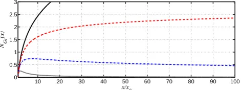
10 20 30 40 50 60 70 80 90 100 0
0.5 1 1.5 2 2.5 3
x/x 0
NG
r
(x)
Fig. 11. Wave amplitude variations versus distance (Eq. 47) for
γ= 1 (black solid line),γ=4/3 (red dashed line),γ=2 (blue dash-dotted line),γ=4 (green dotted line).
from Eq. (47) that the wave amplitude grows up to infinity for γ <4/3, but slower than in the basin of constant depth. In the case of the “non-reflecting” beach (γ=4/3) discussed in Sect. 3, the wave amplitude asymptotically tends to its maximum. For all values γ >4/3, the competition of two effects: resonance and increasing water depth leads to a non-monotonic behavior of the wave amplitude. If the depth increases with distance more rapidly the amplification becomes smaller and the amplification zone becomes narrower.
For analysis to be completed we need to calculate the volume of the landslide. In the case of γ <2 the volume of the landslide can be computed explicitly
MGr(t )=
Z
zb(x,t )dx= Z
c(τ )Q(τ )Z(τ−t )dτ
∼ Z
τ
γ
2(2−γ )Z(τ−t )dτ∼t γ
2(2−γ ). (48)
It increases ast1/2along the plane beach and ast along the “non-reflecting” beach. So, the landslide volume grows with the distance while the wave amplitude decreases forγ >4/3. The second case is the landslide of a constant volume, which height and length vary with a distance. It follows from Eq. (48) that this can be realized ifQ∼c−1:
QC(x)=Q0 h
h0 −1/2
=Q0 x
x0 −γ /2
, (49)
for which
NC(x)=
1 1−3γ /4
h
(x/x0)1−γ−(x/x0)−γ /4
i
, γ6=4/3
ln(x/x0) (x/x0)1/3
, γ=4/3
. (50)
The functionNC(x)is bounded forγ≥1, and for allγ >1 the wave amplitude decreases with the distance (Fig. 12). The maximum amplification along the plane beach (γ=1) isNC(x→ ∞)=4.
10 20 30 40 50 60 70 80 90 100
0 0.5 1 1.5 2 2.5 3
x/x 0
NC
(x)
Fig. 12. Wave amplitude variations versus distance (Eq. 50) for
γ= 1 (black solid line),γ=4/3 (red dashed line),γ=2 (blue dash-dotted line),γ=4 (green dotted line).
10 20 30 40 50 60 70 80 90 100
0 0.5 1 1.5 2
x/x 0
ND
(x)
Fig. 13. Wave amplitude variations versus distance (Eq. 53) for
γ= 1 (black solid line),γ=4/3 (red dashed line),γ=2 (blue dash-dotted line),γ=4 (green dotted line).
And the third case is the landslide motion with the decrease in its volume, which we study on the following example:
QD(x)=Q0 h
h0 −3/4
=Q0 x
x0 −3γ /4
. (51) For the “non-reflecting” bottom profile (10) andZ(τ )defined by Eq. (17) the volume of the landslide can be calculated explicitly.
MD(t )=Q0x0ln
1+ T
τ0+t
. (52)
As before, the wave amplitude is described by the function ND(x)
ND(x)=
1 1−γ
h
(x/x0)1−5γ /4−(x/x0)−γ /4i, γ6=1 ln(x/x0)
(x/x0)1/4, γ
=1 .
(53) Now the wave amplitude decreases for allγ >4/5 including the plane beach (Fig. 13).
6 Conclusions
The tsunami wave generation by submarine landslides of a variable volume moving with a variable speed in a basin of variable depth is studied analytically.
The theory of tsunami wave generation by landslides is developed for basins of “non-reflecting” bottom configura-tionsh∼x4/3 andh∼x4. For such bottom configurations the shallow-water system can be reduced to the constant-coefficient wave equation with an external forcing, and its analytical solution can be expressed in the form of the Duhamel integral. Analytical solutions for tsunami wave generation by landslides of variable volume and speed are obtained and discussed. They consist of three waves: the forced wave propagating in the same direction as the landslide and two free waves propagating in the opposite directions. The forced wave is located above the landslide and propagates with a variable velocity; its length increases with a distance and its amplitude is proportional to the landslide height and decreases with a distance. The forced wave is presented by the wave of elevation in supercritical regime (Fr>1) and by the wave of depression in sub-critical regime (Fr<1). One of the free waves propagates offshore with a variable velocity c(x). It moves behind the landslide in the supercritical regime (Fr>1) and in front of it in sub-critical regime (Fr<1). In the beginning its amplitude increases due to the resonant effect and then decreases according to the Green’s law for the beachh∼x4/3 or stabilizes at deep waters for the beach h∼x4. The wavelengths of the waves propagating offshore increase in time. Another free wave propagates onshore with an increase in its amplitude and decrease in its length.
The runup of the landslide generated wave approaching the coast h∼x4/3 is studied analytically assuming that the wave does not break at the shoreline. The runup characteristics depend on the Froude number.
The process of the resonant generation of tsunami waves by landslides is studied in a basin of slowly varying depth. Using the asymptotic approach, the wave field can be expressed analytically in the integral form. The main result here is that even for the landslide moving with the resonant speed, generally the wave amplitudes remain bounded and decrease at large distances for most of “power-like” beaches. Since the resonance leads to the maximum amplification, the obtained expressions can be used for evaluation of prognostic tsunami waves generated by the submarine landslides of variable volume and speed. These analytical results can also be used for testing numerical schemes.
Acknowledgements. Partial support from the grants by RFBR (08-05-00069, 09-05-91222), EEA (EMP41) and CPER (2010-2013) is gratefully acknowledged. We thank Sebastian Monserrat and two anonymous reviewers for their detailed comments that helped to improve this paper.
Edited by: S. Monserrat
Reviewed by: two anonymous referees
References
Altinok, Y., Tinti, S., Alpar, B., Yalciner, A. C., Ersoy, S., Bortolucci, E., and Armigliato, A.: The tsunami of August 17, 1999 in Izmit Bay, Turkey, Nat. Hazards, 24, 133–146, 2001. Assier-Rzadkiewicz, S., Heinrich, P., Sabatier, P. C., Savoyer, B.,
and Bourillet, J. F.: Numerical modeling of a landslide-generated tsunami: the 1979 Nice event, Pure Appl. Geophys., 157, 1707– 1727, 2000.
Courant, R. and Hilbert, D.: Methods of Mathematical Physics, John Wiley & Sons Inc, 598 pp., 1989.
Deplus, C., Le Friant, A., Boudon, G., Komorowski, J.-C., Villemant, B., Harford, C., S´egoufin, J., and Chemin´ee, J.-L.: Submarine evidence for large-scale debris avalanches in the Lesser Antilles Arc, Earth Planet. Sc. Lett., 192(2), 145–157, 2001.
Didenkulova, I., Pelinovsky, E., Soomere, T., and Zahibo, N.: Runup of nonlinear asymmetric waves on a plane beach, in: Tsunami and Nonlinear Waves edited by: Anjan Kundu, Springer, Germany, 173–188, 2007.
Didenkulova I., Pelinovsky, E., and Soomere, T.: Run-up characteristics of tsunami waves of “unknown” shapes, Pure Appl. Geophys., 165(11/12), 2249–2264, 2008.
Didenkulova, I., Pelinovsky, E., and Soomere, T.: Long surface wave dynamics along a convex bottom, J. Geophys. Res.-Oceans, 114, C07006, doi:10.1029/2008JC005027, 2009.
Didenkulova, I. and Pelinovsky, E.: Traveling water waves along quartic bottom profile, P. Est. Acad. Sci., 59(2), 166–171, doi:10.3176/proc.2010.2.16, 2010.
Didenkulova, I., Pelinovsky, E., and Soomere, T.: Can the waves generated by fast ferries be a physical model of tsunami?, Pure Appl. Geophys., in press, 2010.
Fine, I. V., Rabinovich, A. B., Thomson, R. E., and Kulikov, E. A.: Numerical modeling of tsunami generation by submarine and subaerial landslides, in: Submarine landslides and tsunamis, in NATO Science Series: IV. Earth Env. Sci., 21, edited by: Yalc¸iner, A., Pelinovsky, E., Okal, E., and Synolakis, E., Kluwer, 69–88, 2003.
Fine, I. V., Rabinovich, A. B., Bornhold, B. D., Thomson, R. E., and Kulikov, E. A.: The Grand Banks landslide-generated tsunami of November 18, 1929: preliminary analysis and numerical modeling, Mar. Geol., 215, 45–57, 2005.
Gusiakov, V. K.: Historical Tsunami Database, Natl. Geophys. Data Cent., Novosibirsk, Russia, available at: http://www.ngdc.noaa. gov/hazard/tsu db.shtml (last access: October 2010), 2002. Gusiakov, V. K.: Tsunami history: recorded in The Sea, in:
Tsunamis, edited by: Robinson, A. and Bernard, E., Harvard University Press, Cambridge, 15, 23–54, 2009.
Grimshaw, R., Pelinovsky, D., and Pelinovsky, E.: Homogenization of the variable – speed wave equation, Wave Motion, 47(8), 496– 507, doi:10.1016/j.wavemoti.2010.03.001, 2010.
Imamura, F. and Gica, E. C.: Numerical model for tsunami generation due to subaqueous landslide along a coast, Sci. Tsunami Hazards, 14(1), 13–28, 1996.
Keating, B. H., Waythomas, C. F., and Dawson, A. G.: Landslides and Tsunamis, Pageoph, Topical Volumes, 157, 871–1313, 2000. Liu, P. L.-F., Lynnett, P., and Synolakis, C. E.: Analytical solutions for forced long waves on a sloping beach, J. Fluid Mech., 478, 101–109, 2003.
Mangeney, A., Heinrich, P. H., Rachel, R., Boudon, G., and Cheminee, J.-L.: Modeling of Debris Avalanche and Generated Water Waves: Application to Real and Potential Events in Montserrat, Phys. Chem. Earth Pt. A, 25(9–11), 741–745, 2000. McSaveney, M. J., Goff, J. R., Darby, D. J., Goldsmith, P., Barnett, A., Elliott, S., and Nongkas, M.: The 17 July 1998 tsunami, Papua New Guinea: Evidence and initial interpretation, Mar. Geol., 170, 81–92, 2000.
Kajiura, K.: The leading wave of a tsunami, B. Earthq. Res. Inst. Tokyo, 41, 535–571, 1963.
Kervella, Y., Dutykh, D., and Dias, F.: Comparison between three-dimensional linear and nonlinear tsunami generation models, Theor. Comp. Fluid Dyn., 21, 245–269, 2007.
Kuo, C. Y., Tai, Y. C., Bouchut, F., Mangeney, A., Pelanti,
M., Chen, R. F., and Chang, K. J.: Simulation of
Tsaoling landslide, Taiwan, based on Saint Venant equations over general topography, Eng. Geol., 104(3–4), 181–189, doi:10.1016/j.enggeo.2008.10.003, 2008.
Novikova, L. E. and Ostrovsky, L. A.: Excitation of tsunami waves by a travelling displacement of the ocean bottom, Mar. Geod., 2, 365–380, 1978.
Okal, E. O. and Synolakis, C. E.: Theoretical comparisons of tsunamis from dislocations and slides, Pure Appl. Geophys., 160, 2177–2188, 2003.
O’Loughlin, K. F. and Lander, J. F.: Caribbean Tsunamis, a 500-Year History from 1498–1998, Kluwer Academic Publishers, Netherlands, 263 pp., 2003.
Pelinovsky, E. N.: Hydrodynamics of tsunami waves, Institute of Applied Physics, Nizhny Novgorod, 276 pp., 1996 (in Russian). Pelinovsky, E. N.: Analytical models of tsunami generation by submarine landslides, in: Submarine landslides and tsunamis, NATO Science Series: IV. Earth Env. Sci., 21, edited by: Yalc¸iner, A., Pelinovsky, E., Okal, E., and Synolakis, E., Kluwer, 111–128, 2003.
Pelinovsky, E. and Poplavsky, A.: Simplified model of tsunami generation by submarine landslides, Phys. Chem. Earth, 21, 13– 17, 1997.
Pelinovsky, E., Zahibo, N., Dunkley, P., Edmonds, M., Herd, R., Talipova, T., Kozelkov, A., and Nikolkina, I.: Tsunami Generated by the Volcano Eruption on July 12–13, 2003 at Montserrat, Lesser Antilles, Sci. Tsunami Hazards, 22(1), 44– 57, 2004.
Pudasaini, S. P. and Hutter, K.: Avalanche Dynamics: Dynamics of Rapid Flows of Dense Granular Avalanches, Springer, 602 pp., 2007.
Sammarco, P. and Renzi, E.: Landslide tsunamis propagating along a plane beach, J. Fluid Mech., 598, 107–119, 2008.
Synolakis, C. E.: The runup of solitary waves, J. Fluid Mech., 185, 523–545, 1987.
Synolakis, C. E., Bardet, J., Borrero, J. C., Davies, H. L., Okal, E. A., Silver, E. A., Sweet, S., and Tappin, D. R.: The slump origin of the 1998 Papua New Guinea Tsunami, P. Roy. Soc. Lon. Ser.-A, 458, 763–789, 2002.
Teeuw, R., Rust, D., Solana, C., Dewdney, C., and Robertson, R.: Large Coastal Landslides and Tsunami Hazard in the
Caribbean, EOS T. Am. Geophys. Un., 90(10), 81–88,
doi:10.1029/2009EO100001, 2009.
Ten Brink, U. S., Geist, E. L., and Andrews, B. D.: Size distribution of submarine landslides and its implication to tsunami hazard in Puerto Rico, Geophys. Res. Lett., 33, L11307, doi:10.1029/2006GL026125, 2006.
Tinti, S. and Bortolucci, E.: Analytical investigation of tsunamis generated by submarine slides, Ann. Geofis., 43, 519–536, 2000. Tinti, S., Bortolucci, E., and Chiavettieri, C.: Tsunami excitation by submarine slides in shallow-water approximation, Pure Appl. Geophys., 158, 759–797, 2001.
Ward, S. N.: Landslide tsunami, J. Geophys. Res., 106, 11201– 11215, 2001.
Yalciner, A. C., Pelinovsky, E. N., Okal, E., and Synolakis, C. E.: Submarine landslides and tsunamis, in: NATO Science Series: IV. Earth Env. Sci., Kluwer, 2003.