SRef-ID: 1684-9981/nhess/2005-5-863 European Geosciences Union
© 2005 Author(s). This work is licensed under a Creative Commons License.
and Earth
System Sciences
Validation of Digital Elevation Models around Merapi Volcano,
Java, Indonesia
C. Gerstenecker1, G. L¨aufer1, D. Steineck2, C. Tiede1, and B. Wrobel2
1Institute of Physical Geodesy, Darmstadt University of Technology, Darmstadt, Germany
2Institute of Photogrammetry and Cartography, Darmstadt University of Technology, Darmstadt, Germany
Received: 8 October 2004 – Revised: 19 October 2005 – Accepted: 28 October 2005 – Published: 8 November 2005
Abstract. The accuracy of 4 Digital Elevation Models (SRTM30, GTOPO30, SRTM3 and local DEM produced from aerial photogrammetric images) for the volcanoes Mer-api and Merbabu in Java, Indonesia is investigated by com-parison with 443 GPS ground control points. The study con-firms the high accuracy of SRTM3 and SRTM30, even if the a priori defined 90% confidence level of 16 m for the SRTM3 is not always achieved in this mountainous region. Accuracy of SRTM30, GTOPO30 and SRTM3 is mainly dependent on the altitude itself and the slopes’ inclinations, whereas the pho-togrammetric DEM exhibits constant accuracy over a wide range of altitudes and slopes. For SRTM3 and SRTM30 a statistically significant correlation between heights and as-pects of the slopes is also found.
Accuracy of DEMs which are generated by interpolation on a finer grid does not change significantly. Smoothing of DEMs on a coarser grid, however, decreases accuracy. The decrease in accuracy is again dependent on altitude and slope inclination.
The comparison of SRTM30 with GTOPO30 exhibits a significant improvement of SRTM30 data.
1 Introduction
Accurate and detailed knowledge of topography is basic to many earth processes in- and outside of its surface. Topo-graphic information in the form of Digital Elevation Models (DEM) is used in Geosciences as a tool for reducing and ex-plaining observations as well as for predicting and modeling possible natural hazards such as avalanches, landslides, rock falls or volcanic pyroclastic flows.
Between 1996 and 2002 we participated in the project “MERAPI” (Zschau et al., 1998). One of the most active vol-canoes in the world – Merapi in Central Java, Indonesia – was Correspondence to: C. Gerstenecker
investigated in order to learn how this volcano works and to increase the possibilities of correctly predicting its volcanic activities. In the beginning we immediately realized there was a lack of accurate, up-to-date topographic data. We had available – for our purposes very coarse – the GTOPO30-DEM, bad copies of old topographic maps from 1948, scale 1:25 000 and SPOT images.
A DEM was developed from the SPOT images with a grid size of 20×20 m. However, it has large data gaps due to clouds and smoke development, especially around the sum-mits of Merapi and Merbabu. These gaps were filled by in-terpolation and merging of the digitized contour lines of the topographic maps (Jousset, 1996). Standard deviation – de-termined by comparison with the heights of 360 ground con-trol points – is 121 m (Snitil, 1998).
To improve the situation concerning accuracy and resolu-tion we developed a local DEM – called “LDEM” – from aerial photogrammetric images.
In November 2003 the SRTM3 and SRTM30 DEMs for Europe and Asia were released. We have now the possibility of comparing different DEMs around Merapi to assess accu-racy and resolution of DEMs in tropic mountainous regions. In the following sections we will give more detailed infor-mation about the region under investigation, the DEMs used in this study, the applied statistics, results of the comparisons carried out and final conclusions.
2 The region around Merapi and Merbabu
Fig. 1. Location of the volcanoes Merapi and Merbabu. (a) Map of Indonesia; the red points indicate the locations of active volcanoes. (b) SIR-C/X-SAR- satellite image P-4750 of Central Java taken on October 10, 1994. The volcanoes Ungaran, Telomoyo, Merbabu and Merapi are lined up along a regional fault running NNW-SSE.
The volcanic activities of Merapi are classified as follows: – permanent lava dome development
– periodic dome collapses connected with pyroclastic flows
– lahars at the slopes, especially at the beginning of the rainy season.
The Volcanological Survey of Indonesia (VSI) permanently monitors Merapi’s activities in 5 observatories (Fig. 2).
The region around Merapi and Merbabu is densely popu-lated. Volcanic eruptions of Merapi threaten the city of Yo-gyakarta, located 25 km to the south. Two million people live in and near the so-called forbidden, first and second danger zones.
The elevation range of the region is sizable. Yogyakarta is located at a mean altitude of 100 m a.s.l. The summit of Merbabu is higher than 3100 m a.s.l.
The surface relief around Merapi and Merbabu is very rough. We have analyzed the relief roughness in a region of about 37 km×26 km around Merapi and Merbabu using the relief roughness coefficient RR of Meybeck et al. (2001) RR= hmax−hmin
cs/2 (1)
Fig. 2. Hazard map of Merapi according to Purbawinata et al. (1996).
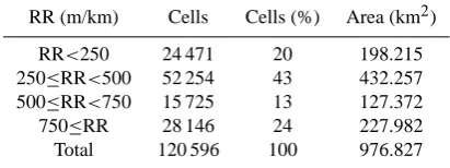
Table 1. Relief Roughness RR around Merapi and Merbabu; cell size=3×300. The computation is based on the SRTM3 – Digital Elevation Model.
RR (m/km) Cells Cells (%) Area (km2)
RR<250 24 471 20 198.215 250≤RR<500 52 254 43 432.257 500≤RR<750 15 725 13 127.372 750≤RR 28 146 24 227.982 Total 120 596 100 976.827
with cs length of cell in kilometers=0.092 km, hmax, hmin maximal and minimal elevation in the cell in meters. For the analysis we used the SRTM3 DEM as described in Sect. 3.1.2.
Inspection of Table 1 shows that relief roughness coeffi-cients RR of 80% of cells are≥250 (m/km). Classification of the topography according to Meybeck et al. (2001) is not meaningful, since more than 80% of the cells are classified as “mountainous, very rough”.
The maximal slope angle reaches 50◦.
and 2600 m vegetation consists of grasses and bushes. Above 2600 m a.s.l. rocks and gravels prevail.
In the following sections we will analyze the accuracy of DEMs between 7◦–8◦S and 110◦–111◦E. Our particular in-terest is focused on a region around Merapi and Merbabu ex-tending 37 km in N-S direction and 26 km in E-W direction.
3 Data
3.1 Digital Elevation Models
In this study we compare 4 of the DEMs currently available for the region around Merapi and Merbabu:
– LDEM – SRTM3 – SRTM30 – GTOPO30
3.1.1 Local Digital Elevation Model LDEM
The local Digital Elevation Model LDEM is a digital sur-face model (DSM), which we have developed from 110 aerial images, image scale 1:50 000. The images were taken in 1981 and 1982. The camera constant is 88 mm, average flight height 5600 m a.s.l.; image overlap along the track of flight is 60%, side lap 20%. The orientation of the im-ages was achieved with the bundle solution using automatic tied point generation and a subset of ground control points (GCPs) (see Sect. 3.2). Grid spacing is 0.5×0.500. LDEM is located between 7◦2001800–7◦4005400S and 110◦1704800– 110◦3202100E and covers an area of 37 km×26 km around Merapi and Merbabu.
Elevations of LDEM are ellipsoidal heights H referenced to the WGS84 ellipsoid (Fig. 3a).
The standard deviation of image coordinates±0.45 pixel as obtained by bundle solution corresponds to±9 m in eleva-tion. That coincides with the anticipated accuracy of LDEM σh≤±8.7 m according to Eq. (2) (Kraus, 2004).
σh≤ ±0.0002∗h+
0.0001
c h∗tanα , (2) where c is camera constant, h flight height above surface
≤5600 m andαslope angle≤50◦. Assuming no systematic errors and normal distribution of the residuals, the a priori accuracy of LDEM is 14.3 m at the 90% confidence interval (Sachs, 1992) according to Eq. (6).
More details about developing LDEM are given by Wrobel et al. (2002) and L¨aufer (2003).
The LDEM-data were also averaged 6×6 to produce 3 arc second data commensurate with SRTM33 (see Sect. 3.1.2). This DEM is referred to as “LDEM33”.
Fig. 3. Local photogrammetric DEM and SRTM3 DEM around Merapi and Merbabu. The color bar gives elevation above sea level (a.s.l.) in meters. Contour line interval is 200 m. (a) Local pho-togrammetric DEM “LDEM”. (b) SRTM3-DEM; the red rectangle in the inset map of Java is the section represented. The magenta dashed rectangle indicates the regions of other DEMs e.g. LDEM, LDEM33, SRTM33 and SRTM0505.
3.1.2 SRTM3
The Shuttle Radar Topography Mission (SRTM) is a joint venture of NASA’s Jet Propulsion Laboratory, National Imaging & Mapping Agency (NIMA), and the German (DLR) and Italian Space Agencies (ASI).
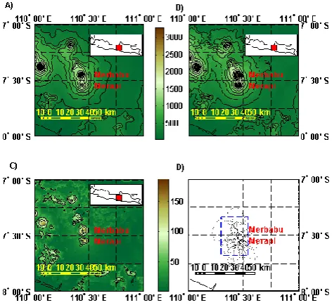
Fig. 4. GTOPO30 and SRTM30 DEMs of Central Java; the red rectangle in the inlet maps of Java gives the range of the DEMs shown; contour line interval is 200 m, unless otherwise noted. (a) GTOPO30 DEM; (b) SRTM30 DEM; (c) Standard deviations of SRTM30 heights of Central Java; contour line interval is 50 m; (d) Ground Control Points GCPs used to determine absolute accuracy of DEMs. The blue dashed rectangle describes the range of the local LDEM.
dual Spaceborne Imaging Radar (SIR-C) and dual X-band Synthetic Aperture Radar (X-SAR) configured as a base-line interferometer (Rosen et al., 2000), acquiring two im-ages simultaneously. These imim-ages, when combined, can produce a single 3-D image. SRTM successfully collected data for 80% of the earth’s land surface, for most of the area between 60◦N and 56◦S latitude (Farr and Kobrick, 2000). SRTM data is being used to generate a digital to-pographic map of the Earth’s land surface with data points spaced every 1 arc second for the United States of America (SRTM1) and 3 arc seconds for global coverage (SRTM3) of latitude and longitude. The linear absolute vertical accu-racy is 16 m, the horizontal circular error 20 m at the 90% confidence level (http://www.nga.mil/ast/fm/acq/890208.pdf MIL-PRF-89020B).
Since November 2003 unedited SRTM3 data have been available under ftp://e0mss21u.ecs.nasa.gov/srtm/. In July 2004 the release was completed with the data of Australia. All this data is specified as being of “research grade”. The data does not meet DTED standards (NIMA, 2000) and has not been edited for voids and spurious height values. Wa-ter bodies often have spurious appearance. In the meantime, “completed” SRTM-Digital Terrain Elevation Data (SRTM DTED) have also been made available on CD at a cost of 60$/CD. A complete overview of all available data can be found at Gamache (2004).
Figure 3b shows the unedited SRTM3-DEM for Central Java between 7◦–8◦S and 110◦–111◦E. The white areas are
due to the data gaps. No data exist for 19 950 cells or 1.4% of the area. Also some cells of the Indian Ocean in the NW corner are not set to 0 m.
Generally any SRTM-DEM is a Digital Surface Model (DSM). That means, the elevation data are with respect to the reflective surface, which may be vegetation, man-made features or bare earth. The elevations h are given above the WGS84 geoid (a.s.l.).
The SRTM dataset, like many other global datasets, has accuracy parameters, which describe it globally, while spe-cific elevation errors are not sufficiently defined.
The C band Interferometric Synthetic Aperture Radar (In-SAR) instrument utilized to collect SRTM data had an inci-dence angle of between 31◦and 61◦thus resulting in slopes of corresponding angles being difficult to image accurately. Mountainous regions such as Merapi and Merbabu are par-ticularly prone to different types of errors with InSAR sys-tems: Layover, shadowing, foreshortening and voids when the slope angle exceeds the incidence of the radar beam (Hansen, 2001; L¨aufer, 2003; Eineder, 2004).
Different validation studies of the SRTM data have been published (see e.g. Heipke et al., 2002; Sarabandi et al., 2002; Smith and Sandwell, 2003; Jarvis et al., 2004a, b; Ko-cak et al., 2004; Falorni et al., 2005) investigating the specific accuracy of SRTM-DEMs.
Generally all authors find that SRTM3 DEMs meet the an-ticipated accuracies of 16 m vertical and 20 m horizontal ac-curacy over flat, open land surfaces. Over terrain with high relief and steep slopes, however, Falorni et al. (2005) suggest that the 16 m stated accuracy specifications should be con-sidered more as guidelines. Gamache (2004) provides a good review of most of the studies. However, no study investigates the accuracy of SRTM3 in mountainous, tropic regions over an elevation range of about 3000 m as we do in this work.
We have derived 3 different DEMs from the original SRTM3 DEM:
– SRTM3F for Central Java between 7◦–8◦S and 110◦– 111◦E is a DEM with 3×300 grid spacing where the voids are filled by interpolation using the shareware software “SRTMFILL” (3D Nature, 2003).
– SRTM33 is a subset of SRTM3F for the same range as LDEM. Grid size is 3×300.
– SRTM0505 has the same range and grid size (0.5×0.500) as LDEM. It is computed by bilinear interpolation of SRTM33 data.
3.1.3 GTOPO30
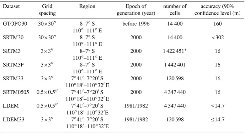
Table 2. Summary of the DEMs analysed.∗Voids are not considered.
Dataset Grid Region Epoch of number of accuracy (90% spacing generation (year) cells confidence level (m)
GTOPO30 30×3000 8–7◦S before 1996 14 400 160 110◦–111◦E
SRTM30 30×3000 8–7◦S 2000 14 400 <302 110◦–111◦E
SRTM3 3×300 8–7◦S 2000 1 422 451∗ 16 110◦–111◦E
SRTM3F 3×300 8–7◦S 2000 1 442 401 16 110◦–111◦E
SRTM33 3×300 7◦410–7◦200S 2000 120 598 16 110◦180–110◦320E
SRTM0505 0.5×0.500 7◦410–7◦200S 2000 4 347 440 16 110◦180–110◦320E
LDEM 0.5×0.500 7◦410–7◦200S 1981/1982 4 347 440 ≤14.7 110◦18’-110◦320E
LDEM33 3×300 7◦410–7◦200S 1981/1982 120 598 ≤14.7 110◦180–110◦320E
The circular accuracy in the DCW is stated as±650 m at the 90% confidence level (USGS-EROS Data Center, 1997), although Gesch et al. (1999) suggest that 160 m linear verti-cal error is more realistic based on comparison with higher resolution sources.
In the following we will analyze only a section of GTOPO30 between 7◦–8◦S and 110◦–111◦E (Fig. 4a). 3.1.4 SRTM30
SRTM30 (Fig. 4b) can be considered to be either a SRTM dataset enhanced with GTOPO30, or an upgrade to GTOPO30. The SRTM3 data were averaged 10×10 to pro-duce 30 arc second data commensurate with GTOPO30. SRTM30 data can be downloaded at no cost from ftp:// e0mss21u.ecs.nasa.gov/srtm/. Instead of a 90% confidence level, the standard deviation of each cell is provided. Fig-ure 4c shows the SRTM30 standard deviations for Central Java between 7◦–8◦S and 110◦–111◦E. The maximum stan-dard deviation is 189 m.
Standard deviations of cells of altitudes <500 m are <±20 m. The largest standard deviations are found at the summits of volcanoes e.g. Merapi and Merbabu.
3.2 Ground control points
Between 1996 and 2002 we carried out repeated gravity mea-surements around Merapi and Merbabu (Gerstenecker et al., 1998; Setiawan, 2003; Tiampo et al., 2004; Jentzsch et al., 2004; Tiede et al., 2005). For the positioning of gravity points geodetic Trimble and Leica GPS receivers were uti-lized. Least square adjustments of the GPS-observations with the software packages GPSurvey 3.5 (Division, 1995) and “Bernese 4.2” (Hugentobler et al., 2001) yield identical results. The root mean square errors (RMSE) for the
horizon-tal coordinates are <±0.1 m and for the vertical <±0.2 m (G¨otz, 2003). Horizontal accuracy at the 90% confidence level is 0.16 m, the vertical 0.32 m.
In total we have determined the 3-D coordinates of 443 points in the International Terrestrial Reference Frame 2000 (Boucher et al., 2004). We use them in the following as Ground Control Points (GCPs) (Fig. 4d).
The coordinates of the GCPs are given on the WGS84 el-lipsoid. The elevations H are ground truth ellipsoidal heights. In order to convert them to heights h above sea level (a.s.l.) the geoid heights N are subtracted according to Eq. (3) (Heiskanen and Moritz, 1967)
h=H−N . (3)
Global geoid heights with 2×20 grid spacing calculated
from the Earth Gravity Model 96 (EGM96) (Lemoine et al., 1997) are currently available from http://topex.ucsd.edu/ cgi-bin/get data.cgi.
Table 2 provides a summary of the data described in Sect. 3. One important criterion for the following investi-gation is the period in which the data of the DEMs are col-lected. Changes in geomorphology and vegetation in tropic, volcanic regions occur very quickly and have to be consid-ered if different DEMs in such regions are compared.
4 Statistics
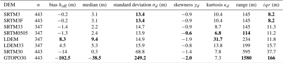
compari-Table 3. Statistics for the different DEMs;n=number of available ground control points (GCP);iqr=interquartile range. Extreme values are marked by bold numbers.
DEM n biashoff(m) median (m) standard deviationσd(m) skewnessγd kurtosisκd range (m) iqr(m)
SRTM3 443 −0.2 3.1 13.4 −0.9 10.4 145 8.2
SRTM3F 443 −0.2 3.1 13.4 −0.9 10.4 145 8.2
SRTM33 347 −1.4 2.2 14.7 −0.9 8.7 145 11.3
SRTM0505 347 −1.3 2.4 13.9 −0.6 6.8 114 11.2
LDEM 347 8.3 9.4 14.9 −1.9 31.7 234 11.8
LDEM33 347 4.5 5.3 15.9 −0.8 13.8 199 15.7
SRTM30 443 −14 0.3 68.8 −1.4 7.8 595 37.7
GTOPO30 443 −102.5 −38.5 249.2 −2.0 7.3 1580 166
son with other DEMs of higher accuracy (Koch and Heipke, 2001; Muller et al., 2000; Jarvis et al., 2004a, b).
Relative accuracy of a DEM is assessed by comparing it with a reference DEM of the same extension and grid size.
To estimate absolute accuracy, elevationshDEM at the lo-cations of GCPs were extracted from all DEMs and com-pared with the elevations of GCPshGCPin order to determine the differencesdi, biashoff, residualsvi, standard deviation
σd, skewnessγd, kurtosisκdand range according to Eq. (4)
di =hDEM−hGCP hoff= 1n
n
P
i=1 di
vi =di −hoff
σd=
s n
P
i=1
vi2 n−1 γd =
E
v3
i
σd3
κd = E
v4
i
σd4
range=vmax−vmin
(4)
wheren is number of samples andE mathematical expec-tation. Additionally we give the median (50th percentile) of the differencesdi and the interquartile rangeiqr – the
dif-ference between the 75th and 25th percentile of the residuals vi. Scatter plots ofvi overhGCP represent the dependence of residualsvi from elevationshGCP. Histograms show the distribution of residualsvi of the particular DEMs.
Residualsvi of all DEMs are binned into different classes
depending on heighthGCP, slopeαGCP and aspectAGCP at GCP locations. Biases and standard deviations for each class are computed and plotted againsthGCP, slopeαGCPand as-pectAGCP, respectively.
The relative accuracy between two Digital Elevation Mod-els DEM1 and DEM2 of identical grid size is evaluated in a similar way. Instead of hGCP, the heights of a second DEMhDEM2 are used as reference. The differencesdri of
the heightsh,dAi of the aspectsAanddαi of the slopesα,
respectively, are computed using Eq. (5). dri =hDEM1−hDEM2
dAi =ADEM1−ADEM2 dαi =αDEM1−αDEM2
(5)
Biashoff, residualsvi, standard deviationσd, skewness γd
and kurtosisκdare estimated by inserting the differencesdri,
dAi anddαiinstead ofdi in Eq. (4).
Residualsvi are binned again in different classes
depen-dent on heighthDEM2, slopeαDEM2and aspectADEM2.
5 Results
5.1 Absolute accuracy of DEMs from ground control points
Elevation values were extracted from all DEMs and com-pared with the GCPs-heights in order to determine the pa-rameters according to Eq. (4). The results of the comparison are summarized in Table 3.
Inspection of Table 3 shows that the interpolation of gaps in SRTM3 does not influence the absolute accuracy. There-fore, in the following we provide results only for SRTM3F and all offsprings, e.g. SRTM33 and SRTM0505.
The residualsvi of the DEMs do not have a normal
distri-bution, since skewnessγd is always6=0. Some of the
distri-bution histograms are plotted as examples in Fig. 5a–5d. In the literature there are no hints indicating for which distribution the 90% confidence level of SRTM3 is defined. If we assume normal distribution, the 90% confidence level is related to the standard deviationσd according to Eq. (6)
(Sachs, 1992)
P (|vi| ≥1.645σd)≤0.1. (6)
The a priori standard deviationσdof SRTM3 is then≤10 m.
Otherwise Tschebyscheff’s inequality P (|vi| ≥kσd)≤
1
k2 (7)
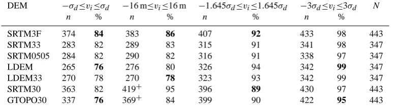
Table 4. Number of samplesvi within different error bounds. N is the number of all available GCPs (100%),nthe number of samples,
whereviis within the error margins. Extreme values are marked by bold numbers.+For SRTM30 and GTOPO30 a 90% confidence interval
−160 m≤σ≤160 m is assumed.
DEM −σd≤vi≤σd −16 m≤vi≤16 m −1.645σd≤vi≤1.645σd −3σd≤vi≤3σd N
n % n % n % n %
SRTM3F 374 84 383 86 407 92 433 98 443 SRTM33 283 82 289 83 315 91 341 98 347 SRTM0505 284 82 290 82 316 91 338 97 347
LDEM 265 76 276 80 326 94 342 99 347
LDEM33 270 78 270 78 323 93 342 99 347 SRTM30 363 82 419+ 95 396 89 430 97 443 GTOPO30 337 76 369+ 84 399 90 422 95 443
– σd≤vi≤σd,
– 16 m≤vi≤16 m,
– 1.645σd≤vi≤1.645σd,
– 3σd≤vi≤3σd.
The number of samples within the –σd≤vi≤σderror margin
exceeds the limits of normal distributed samples of 68% sig-nificantly. However, none of the DEMs in Table 4 meets the a priori defined 90% confidence level of 16 m (see Sect. 3.1). The residuals of all DEMs are within the 90% confidence interval, if Eqs. (6) or (7) is applied.
For analyzing the influence of outliers we computed the statistics according to Eq. (4), with which we have eliminated outliers before. In Tables 5–7 the statistics for the different error margins are shown.
SRTM3F generally has the smallest standard deviation. For the accuracy investigation of SRTM3F, 443 GCPs are available compared to 347 for SRTM33 and LDEM. Each of these additional 96 GCPs are located at altitudes between 100 m and 1000 m, the elevation range where SRTM data fit within the 90% confidence level of 16 m with GCPs heights. After SRTM3F, standard deviation of LDEM has the smallest value (Tables 5–7).
Depending on the number of deleted outliers, interpolation of SRTM33 on a finer grid of 0.5×0.500 decreases the
stan-dard deviationσdup to 6.6%; averaging of LDEM on a 3×300
grid increasesσdby more than 25% (Tables 5–7).
In Figs. 5e and 5f the residualsvi of LDEM and SRTM33
are plotted over GCP heightshGCP. The plot exhibits two important features:
– LDEM residuals are <0 in the range between 100 m≤hGCP≤500 m. Above 500 m the dispersion of the residuals is low. There, LDEM heights are larger than GCP heights.
– SRTM33 residuals show small variations between 100 m≤hGCP≤1000 m. The dispersion increases with increasinghGCP.
Fig. 5. Histograms and scatter plots of height differences di:
Table 5. Statistics for 90% confidence level: outliers|vi|≥3×σdare not considered;n=number of analyzedvi;iqr=interquartile range.
Extreme values are marked by bold numbers.
DEM n biashoff(m) median (m) standard deviationσd(m) skewnessγd kurtosisκd range (m) iqr(m)
SRTM3F 433 0.4 3.1 10.5 −1.3 6.0 76 7.6
SRTM33 341 −41.1 2.3 12.3 −1.2 5.1 81 10.8
SRTM0505 338 −0.7 2.6 11.5 −1.0 4.7 74 10.9
LDEM 342 8.7 9.4 9.6 −0.1 5.1 77 10.7
LDEM33 342 4.7 5.3 12.8 −0.2 4.0 88 15.3
SRTM30 430 −7.7 1.0 54.2 −0.7 6.1 395 32.5
GTOPO30 422 −61.4 −27.8 170.5 −1.4 6.4 1197 150.3
Table 6. Statistics for 90% confidence level: outliers|vi|≥1.645×σdare not considered;n=number of analyzedvi;iqr=interquartile range.
Extreme values are marked by bold numbers.
DEM n biashoff(m) median (m) standard deviationσd(m) skewnessγd kurtosisκd range (m) iqr(m)
SRTM3F 407 1.8 3.3 7.4 −1.0 4.6 44 6.6
SRTM33 315 0.9 2.9 8.4 −0.8 3.8 47 8.7
SRTM0505 316 0.6 2.8 8.4 −1.0 3.8 46 9.3
LDEM 326 7.7 9.1 8.0 −0.7 3.5 43 10.5
LDEM33 323 4.1 5.1 10.6 −0.4 3.0 51 14.9
SRTM30 396 −1.9 1.9 33.8 −0.3 4.5 215 28.3
GTOPO30 399 −34.4 −22.9 119.3 −0.4 4.2 754 128
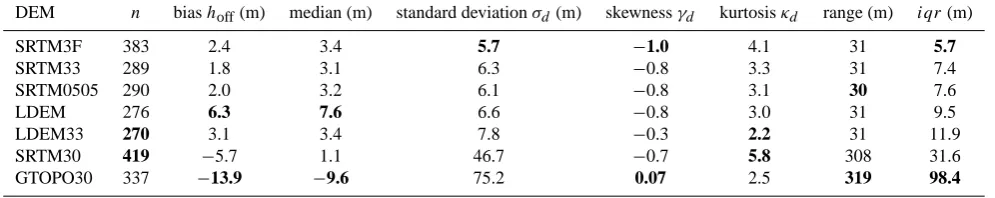
Table 7. Statistics: residuals|vi|>16 m are not considered;n=number of analyzedvi,iqr=interquartile range. Extreme values are marked
by bold numbers.
DEM n biashoff(m) median (m) standard deviationσd(m) skewnessγd kurtosisκd range (m) iqr(m)
SRTM3F 383 2.4 3.4 5.7 −1.0 4.1 31 5.7
SRTM33 289 1.8 3.1 6.3 −0.8 3.3 31 7.4
SRTM0505 290 2.0 3.2 6.1 −0.8 3.1 30 7.6
LDEM 276 6.3 7.6 6.6 −0.8 3.0 31 9.5
LDEM33 270 3.1 3.4 7.8 −0.3 2.2 31 11.9
SRTM30 419 −5.7 1.1 46.7 −0.7 5.8 308 31.6
GTOPO30 337 −13.9 −9.6 75.2 0.07 2.5 319 98.4
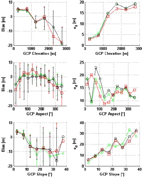
We have binned the residuals vi in different classes
de-pending on heighthGCP, aspectAGCPand slopeαGCPat the GCP locations in order to investigate the regression of biases and standard deviations on GCP heights, aspects and slopes. Number of samples/class is shown in Table 8.
In Figs. 6–8 class biases and class standard deviations are plotted for the different DEMs.
The SRTM-class biases and standard deviations change nonlinearly with height hGCP (Fig. 6): Up to 1000 m a.s.l. class biases are >0 m; the dispersions of the residuals are small. The standard deviations confirm that the data are quite well within the 90% confidence interval of 16 m. Above 1000 m a.s.l. the SRTM-biases become<0 m. Standard de-viations increase significantly.
Similar behavior shows the plot of biases and standard deviations over the slope α (Fig. 6). For slopes between 0◦<α<10◦we find biases≥0 m and standard deviations be-tween 6 and 10 m. For slopesα>10◦the biases are<0 m and the standard deviations increase up to 35 m.
There also seems to be a correlation between aspect A and the class biaseshoff. Biases hoff reach at aspects between 100◦and 150◦a maximum.
The photogrammetric LDEM exhibits homogenous accu-racy (red lines in Fig. 7). Standard deviation σd decreases
Fig. 6. Class biases hoff and standard deviationsσd of SRTM3F, SRTM33 and SRTM0505 heights plotted over GCP elevations, aspects and slopes. Error bars of class biases are 3σ er-ror bars. Red lines=SRTM0505 biases and standard devia-tions; green lines=SRTM 3F biases and standard deviadevia-tions; blue lines=SRTM33 biases and standard deviations.
Class biases of LDEM33 (blue lines in Fig. 7) differ for heightshGCP>1000 m from LDEM-class biases. Class stan-dard deviations of the LDEM33vi increase withhGCP. They are generally larger than LDEM class standard deviations.
Figure 8 demonstrates that class biases of GTOPO30 and SRTM30 become smaller with increasing hGPC and slopeαGCP; however, the class standard deviations increase. SRTM30 heights fit hGCP much better than GTOPO30 heights even at high altitudes. Biases of GTOPO30 heights are strongly dependent on aspectAGCP.
The locations of GCPs whose residualsvi exceed the
er-ror bound−16 m≤vi≤16 m are plotted in Fig. 9. For LDEM
most of these points are located on the western slopes of Mer-api, whereas the outliers for SRTM-DEMs are distributed more randomly on the eastern slopes of Merbabu and Mer-api.
5.2 Relative accuracy of DEMs
In this section we estimate the relative accuracy between SRTM DEMs and LDEM as well as between SRTM30 and GTOPO30. The aim is to identify areas with systematic dif-ferences between the particular DEMs. The large number of samples (cells) allows the estimation of reliable
statis-Fig. 7. Class biases hoff and standard deviationsσd of LDEM
and LDEM33 plotted over GCP heights, aspects and slopes. Er-ror bars of class biases are 3σ error bars. Red lines=LDEM biases and standard deviations; blue lines=LDEM33 biases and standard deviations.
tics. For this study we use all LDEM-models and GTOPO30 as reference models (hDEM2, ADEM2,αDEM2)according to Eq. (5).
5.2.1 Comparison between SRTM3 and LDEM Comparisons were carried out in 2 ways:
– comparison of DEM heights, – comparison of aspects and slopes. Two pairs of DEMs were compared:
– SRTM33 – LDEM33, – SRTM0505 – LDEM.
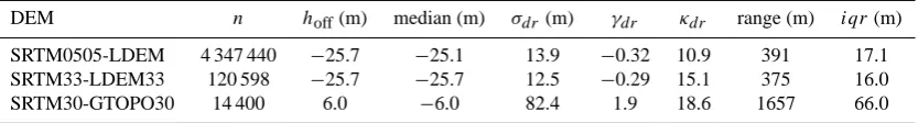
Results are given in Table 9. The biases hoff between SRTM33 and LDEM33 as well as SRTM0505 and LDEM correspond well with the mean geoid height of −25.7 m. Again the residuals vi are not distributed normally, since
skewness γd is 6=0. Standard deviations σd vary between
Table 8. Binning of residualsviof investigated DEMs dependent on height, aspect and slope at GCP locations; numbers are the samples/class.
Classification SRTM 3F SRTM 33 SRTM 0505 LDEM33 LDEM SRTM 30 GTOPO 30
HeighthGCP
h≤500 107 32 32 29 29 107 107
500<h≤1000 127 106 106 101 99 127 127 1000<h≤1500 107 107 107 103 101 107 107
1500<h≤2000 55 55 55 48 49 55 55
2000<h≤2500 21 21 21 21 23 21 21
2500<h 26 26 26 21 25 26 26
AspectAGCP
0◦<A≤30◦ 21 18 18 12 15 12 12
30◦<A≤60◦ 21 17 25 19 24 20 20
60◦<A≤90◦ 27 17 15 20 19 48 48
90◦<A≤120◦ 48 32 33 25 28 86 86
120◦<A≤150◦ 52 38 37 43 46 52 52
150◦<A≤180◦ 53 41 38 38 42 61 61
180◦<A≤210◦ 61 41 40 38 33 39 39
210◦<A≤240◦ 44 40 51 32 30 44 44
240◦<A≤270◦ 40 36 24 31 24 46 46
270◦<A≤300◦ 32 30 29 34 25 15 15
300◦<A≤330◦ 21 17 20 13 20 10 10
330◦<A≤360◦ 23 20 16 18 20 10 10
SlopeαGCP
α≤5◦ 209 114 114 100 100 225 225
5◦<α≤10◦ 95 101 101 104 104 158 158
10◦<α≤15◦ 39 37 37 35 35 33 33
15◦<α≤20◦ 38 26 26 33 33 2 2
20◦<α≤25◦ 30 27 27 25 25 18 18
25◦<α≤30◦ 13 21 21 11 11 5 5
30◦<α≤35◦ 15 13 13 11 11 2 2
35◦<α 4 4 4 4 4 0 0
Table 9. Statistics of height differencesdr;nis the number of samples,hoffthe bias,σdrthe standard deviation,γdr skewness,κdr the
kurtosis andiqrthe interquartile range, respectively.
DEM n hoff(m) median (m) σdr(m) γdr κdr range (m) iqr(m)
SRTM0505-LDEM 4 347 440 −25.7 −25.1 13.9 −0.32 10.9 391 17.1 SRTM33-LDEM33 120 598 −25.7 −25.7 12.5 −0.29 15.1 375 16.0 SRTM30-GTOPO30 14 400 6.0 −6.0 82.4 1.9 18.6 1657 66.0
Additional information gives the plot of the residualsvi in
Fig. 9. The residuals at heights up to 600 m a.s.l. are>0 m. They become<0 m with elevations>600 m.
If we assume 16 m as 90% confidence level for both DEMs, the 90% confidence levelcl for the residualsvi
ac-cording to the error propagation law is cl=16∗
√
2=22.6 m (8)
Cells where the residualsvi≤−22.6 andvi≥22.6 are shown
in Fig. 9 as magenta and white areas, respectively. The
largest magenta area is located at the western foot of Mer-api’s slopes. According to the aerial images taken in 1981 and 1982 this area was covered by rain forest. In 1996, when we visited this area for the first time, the forest had been re-placed by low shrubbery and grass. Perhaps these residuals reflect the change of vegetation.
White areas are located at the south-eastern and north-western corners of LDEM33.
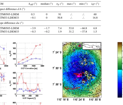
Table 10. Statistics of aspect differencesdAand slope differencesdα. hoffis the bias,σdthe standard deviation andiqrthe interquartile
range, respectively.
DEM hoff(◦) median (◦) σd(◦) max (◦) min (◦) iqr(◦)
Aspect differencedA(◦)
SRTM0505-LDEM 0.3 0 91 ./. ./. 60 SRTM33-LDEM33 −0.1 0 50.8 ./. ./. 16.8 Slope differencedα(◦)
SRTM0505-LDEM −3.9 −1.7 7.4 53.0 −66.8 6.8 SRTM33-LDEM33 −0.3 −0.2 1.9 31.2 −37.8 1.5
Fig. 8. Class biases hoff and standard deviations σd of
SRTM30 and GTOPO30 heights plotted over GCP heights, as-pects and slopes. Error bars of class biases are 3σ error bars. Red lines=GTOPO30 biases and standard deviations; blue lines=SRTM30 biases and standard deviations.
aspectALDEMand slopeαLDEM(Fig. 10). Absolute values of class biases and standard deviations increase with increasing altitude and slope. Class biases reach maximum values at aspects ofA=135◦and 245◦.
5.2.2 Comparison of aspects and slopes
AspectAand slopeαare the first derivatives of a DEM. We computed them in order to assess how well topographic de-tails are represented in the different DEMs. In Table 10 we show the basic statistics of the differencesdAi anddαi
ac-cording to Eq. (5).
Fig. 9. Residualsvi=SRTM33 elevations – LDEM33 elevations;
the color bar gives the residualsvi in meters; contour lines show
topography; contour line interval is 200 m; magenta areas are re-gions where residualsvi<−22.6 m, white areas are regions, where
residualsvi>22.6 m; red circles are GCPs where the residuals
be-tween LDEM33 and GCP elevations exceed the 90% confidence level (±20.4 m); yellow squares are the GCPs, where the residuals vi between SRTM33 and GCP elevations exceed the 90%
confi-dence level (±20.2 m).
There is no significant bias concerning the aspects. Slope biases are small, whereby LDEM slopes are in the mean larger than SRTM slopes. Generally, dispersion parameters such as standard deviation, range and interquartile range iqr for the coarse grid DEMs (SRTM33 and DEM33) are smaller than for the fine grid DEMs. Therefore, the coarse grid DEMs (SRTM33 and DEM33) fit each other better than the fine grid DEMs (LDEM and SRTM0505).
LDEM and DEM33 contain considerably more topo-graphic details than SRTM33 and SRTM0505. As an exam-ple, gradients of topography around the summit of Merapi are shown in Fig. 11.
Fig. 10. Class biaseshoffand standard deviationsσdof SRTM0505
and SRTM33 heights over LDEM and LDEM33 heights, as-pects and slopes. Error bars of class biases are 3σ error bars. Red lines=SRTM0505 biases and standard deviations; blue lines=SRTM33 biases and standard deviations.
Fig. 11. Topographic details of Merapi summit. Contour line inter-val is 200 m. Blue arrows show topography’s gradients. Dashed black lines are topographic edges and ridges as determined by Canny’s algorithm (Canny, 1986). Red markers give the location of the GCPs at the summit. (a) LDEM; (b) SRTM0505; (c) LDEM33; (d) SRTM33.
Fig. 12. Height differences between SRTM30 and GTOPO30 heights. Contour lines give the topography. Contour line interval is 500 m. The circles mark the locations of GCPs. (a) Height differ-ences between SRTM30 and GTOPO30 heights. The blue dashed rectangle gives the range, which is shown in more detail in (b)–(d). (b) Height differences around the summits of Merapi and Merbabu. (c) Detail of SRTM30 DEM around the summits of Merapi and Merbabu. (d) Detail of GTOPO30 DEM around the summits of Merapi and Merbabu.
the algorithm by Canny (1986). With the Canny approach in LDEM many topographic structures are identified. We can check their accuracy using the horizontal positions of the ground control points. Most of the GCPs plotted in Fig. 11 are located very near to ridges and break lines, where they also are in nature (Wrobel et al., 2002).
Ridges and break lines as generated from SRTM33, SRTM0505 and LDEM33 by the Canny algorithm are not correct. Obviously the grid spacing of SRTM33 and LDEM33 is too coarse to render small scale details of the topography.
5.2.3 SRTM30 – GTOPO30
The differencesvi between SRTM30 and GTOPO30 are
un-usually large (Table 9, Fig. 12a). The distribution of residu-alsvi shows some systematic behaviour. The minimum and
maximum of residualsvi are found around the summits of
Fig. 13. Class biaseshoffand standard deviationsσdof SRTM30
heights over GTOPO30 heights, aspects and slopes. Error bars of class biases are 3σerror bars.
xo andyoshould also be determined with the help of a
3-dimensional similarity transformation (Heipke et al., 2002). Class biaseshoffand class standard deviationsσdincrease
with elevations and slopes. Class biases are also dependent on aspects, where the extreme values are found at aspects of 75◦and 255◦(Fig. 13). Primarily the circular errors are responsible for the dependencies of residuals on aspect and the increase of class biases with elevation and slope.
6 Conclusions
This study provides a broad range of results on the accuracy of investigated DEMs. Generally we can show that SRTM-3 and SRTMSRTM-30 are a vast improvement on previous global DEM products.
However, the biases and standard deviations of the DEMs analysed are nonlinearly dependent on elevations and slopes. Through comparison with GCPs we find that standard de-viation of SRTM3 DEMs increases with elevation and slope, whereas bias shows nonlinear changes. The specified 90% confidence level of 16 m is exceeded when absolute heights are>1000 m. Up to an elevation of 1000 m the SRTM data satisfy the 90% confidence level.
The photogrammetric LDEM data displays accuracy sim-ilar to SRTM3. Class biases also change with altitude. How-ever, class standard deviations decrease with elevation.
LDEM data represent more topographic details than SRTM3, e.g. break lines and ridges. This is also true if LDEM data are averaged on the coarser grid size of SRTM3. Averaging decreases accuracy. Interpolation of SRTM3 data on a finer grid possibly decreases standard deviation. How-ever, interpolation cannot improve the topographic details.
The DEMs generated by the SRTM mission are a sub-stantial and very significant step towards detailed accurate global DEMs, especially for far, remote and poorly surveyed regions.
SRTM30 is an excellent replacement of the inhomoge-neous GTOPO30, particularly in mountainous regions like the volcanic area around Merapi and Merbabu.
However, SRTM3 does not make the generation of local, high resolution DEMs unnecessary. Such models are only generated by special missions (laser scanning, large scale aerial photogrammetric images, airborne SAR) dedicated to the determination of a high resolution, highly accurate DEM.
Acknowledgements. Research has been partly supported by the
German Research Society under project no. GE 381/12 1-4. The authors thank M. Hovenbitzer and F. Guzzetti for their help in improving this study significantly.
Edited by: M. Jaboyedoff
Reviewed by: F. Guzzetti and M. Hovenbitzer
References
3D Nature: SRTMFILL, http://www.3dnature.com/srtmfill.html, 2003.
Boucher, C., Altamimi, Z., Sillard, P. and Feissel-Vernier, M.: The ITRF2000, IERS Technical Note, 31, Verlag des Bundesamtes f¨ur Kartographie und Geod¨asie, Frankfurt am Main, 2004. Canny, J.: A computational approach to edge detection, IEEE
Transactions on Pattern Analysis and Machine Intelligence, Vol. PAMI 8, 679–698, 1986.
Danko, D. M.: The digital chart of the world, Geoinfo Systems, 2, 29–36, 1992.
Division, S. M.: GPSurvey Software User’s Guide, Sunnyvale, CA 94088-3642, USA, 1995.
Eineder, M.: Problems and solutions for INSAR digital eleva-tion models generaeleva-tion of mountainous terrain, Proceedings of FRINGE Workshop, Frascati, 1–5 December 2003, ESA SP-550, June 2004.
Falorni, G., Teles, V., Vivoni, E. R., Bras, R. L., and Amaratunga, K. S.: Analysis, characterization and effects on hydrogeomor-phic modeling of the vertical accuracy of Shuttle Radar Topog-raphy Mission digital elevation models, J. Geophys. Res. – Earth Surface, in press, 2005.
Farr, T. G. and Kobrick, M.: Shuttle Radar Topographic Mission produces a wealth of data, EOS, Transactions, American Geo-physical Union, 81, 583–585, 2000.
Gamache, M.: Free and low cost datasets for international mountain cartography, http://www.icc.es/workshop/abstracts/ ica paper web3.pdf, 2004.
1. Merapi-Galeras Workshop Potsdam, 25 June 1998, Deutsche Geophysikalische Gesellschaft, Sonderband III, 1998.
Gesch, D. B., Verdin, K. L., and Greenlee, S. K.: New land surface digital elevation covers the earth, EOS, Transactions, American Geophysical Union, 80, 69–70, 1999.
G¨otz, C.: Auswertung und Deformationsanalyse von GPS-Messungen am Vulkan Merapi auf Java, Indonesien, Diplom Thesis, Institute of Physical Geodesy, Darmstadt University of Technology, 2003.
Hansen, R. F.: Radar Interferometry. Data interpretation and anal-ysis. Kluwer Academic Publishers, Dordrecht, The Netherlands, 2001.
Heipke, C., Koch, A., and Lohmann P.: Analysis of SRTM DTM-Methodology and practical results, Swedish Photogrammetric Journal Bildteknik/Image Science, No. 2002:1, April 2002. Heiskanen, W. A. and Moritz, H.: Physical Geodesy, W. H.
Free-man and Co., San Francisco and London, 1967.
Hugentobler, U., Schaer, S., and Fridez, P. (eds.): Bernese GPS soft-ware version 4.2, Astronomical Institute, University of Berne, 2001.
Jarvis, A., Rubiano, J., and Cuero, A.: Comparison of SRTM de-rived DEM vs. topographic map dede-rived DEM in the region of Dapa, http://gisweb.ciat.cgiar.org/sig/download/laboratory gis/srtm vs topomap.pdf, 2004a.
Jarvis, A., Rubiano, J., Nelson, A., Farrow, A., and Mulligan, M.: Practical use of SRTM data in the tropics – comparisons with digital elevation models generated from cartographic data, In-ternational Center for Tropical Agricultura, Working Document, no. 198, 2004b.
Jentzsch, G., Weise, A., Rey, C., and Gerstenecker, C.: Gravity changes and internal processes: some results obtained from ob-servations at three volcanoes, Pure and Applied Geophysics, 161, 1415–1431, 2004.
Jousset, P.: Structure et Dynamisme du Volcan Merapi, Indonesie, PhD thesis, Universite VII, IPGP Paris, 1996.
Kocak, G., B¨uy¨uksalih, G., and Jacobsen, K.: Analysis of digital elevation models determined by high resolution space images, IntArchPhRS, Band XXXV, Teil B4, 636–641, Istanbul, 2004. Koch, A. and Heipke, C.: Quality Assessment of Digital Surface
Models derived from the Shuttle Radar Topography Mission (SRTM), Proceedings of IGARSS, Sydney, Australia, Supple-ment CD, 2001.
Kraus, K.: Photogrammetrie, Band 3, Topographische Information-ssysteme. D¨ummler, K¨oln, 2000.
Kraus, K.: Photogrammetrie, Band 1, Geometrische Informatio-nen aus Photographien und Laserscanneraufnahmen, 7. Auflage, Walter de Gruyter, Berlin, New York, 2004.
L¨aufer, G.: Erzeugung hybrider digitaler H¨ohenmodelle aktiver Vulkane am Beispiel des Merapi, Indonesien, PhD thesis, Darm-stadt University of Technology, Aachen, 2003.
Lemoine, F. G., Smith, D. E., Kunz, L., Smith, R., Pavlis, E. C., Pavlis, N. K., Klosko, S. M., Chinn, D. S., Torrence, M. H, Williamson, R. G., Cox, R. G., Rachlin, K. E., Wang, Y. M, Kenyon, S. C., Salman, R., Trimmer, R., Rapp, R. H., and Nerem, R. S.: The development of the NASA GSFC and NIMA joint geopotential model, in: Gravity, Geoid and Marine Geodesy, edited by: Segawa, J., Fujimoto, H., and Okubo, S., International Association of Geodesy Symposia, 117, 461–469, 1997.
Meybeck, M., Green, P., and V¨or¨ormart, C.: A new typology for mountains and other relief classes: An application to global wa-ter resources and population distribution, Mountain Research and Development, 21, 34–45, 2001.
Muller, J. P., Morley, J. G., Walker, A. H., Kitmitto, K., Mitchell, K. L., Chugani, K., Smith, A., Barnes, J., Keenan, R., Cross, P. A., Dowman, I. J., and Quarmby, N.: The LANDMAP project for the automated creation and validation of multiresolution or-thorectified satellite image products and a 1” DEM of the British isles from ERS tandem SAR interferometry, LANDMAP Special Session, RSS200, Leicester University, http://www.landmap.ac. uk/docs/RSS00 JPM paperV1.pdf, 2000.
NIMA: Performance specification Digital Terrain Elevation Data (DTED), http://www.nga.mil/ast/fm/acq/890208.pdf, 2000. Purbawinata, M. A., Ratdomopurbo, A., Sinulingga, I. K., Sumarti,
S., and Suharno, I.: Merapi volcano – guide book, Volcanologi-cal Survey of Indonesia, Bandung, 1996.
Rosen, P. A., Hensley, S., Joughin, I. R., Li, F. K., Madsen, S. N., Rodriguez, E., and Goldstein, R. M.: Synthetic aperture Radar interferometry, Proceedings IEEE, 88, 333–382, 2000.
Sachs, L.: Angewandte Statistik, 7. Auflage, Springer, Berlin, Hei-delberg, New York, 1992.
Sarabandi, K., Brown, C. G., Pierce, L., Zahn, D., and Azadegan, R.: Calibration validation of the SRTM height data for Southeast-ern Michigan, 2002 IEEE Geoscience and Remote Sensing Sym-posium (IGARSS’02), Toronto, Canada, Vol. I, 167–169, 2002. Setiawan, A.: Modeling of gravity changes on Merapi volcano
ob-served between 1997–2000, PhD thesis, Darmstadt University of Technology, 2003.
Smith, B. and Sandwell, D.: Accuracy and resolution of shuttle radar topography mission data, Geophys. Res. Lett., 30, 9, 1467– 1470, 2003.
Snitil, B.: Erstellung eines digitalen Gel¨andemodells aus ver-schiedenen Datenquellen, Diplom thesis, Institute of Physical Geodesy, Darmstadt University of Technology, 1998.
Tiampo, K., Fern´andez, J., Jentzsch, G., Charco, M., Tiede, C., Gerstenecker, C., Camacho, A., and Rundle, J.: Elastic – gravita-tional modelling of geodetic data in active volcanic areas, Recent Research Development in Geophysics, 6, 37–58, 2004.
Tiede, C., Tiampo, K., Fern´andez, J., and Gerstenecker, C.: Deeper understanding of non-linear geodetic data inversion using quanti-tative sensitivity analysis, Nonlin. Processes Geophys., 12, 373– 379, 2005,
SRef-ID: 1607-7946/npg/2005-12-373.
USGS-EROS Data center: GTOPO30 documentation (README file), in: Land Processes Distributed Active Archive Center, http: //edcdaac.usgs.gov/gtopo30/README.asp, 1997.
Van Bemmelen, R. W.: The influence of geological events on hu-man history (an example from central Java), Verh. Kon. Ned. Geol. Mijnb. Genoot. Geol., 16, 20–36, 1956.
Wrobel, B. P., Gerstenecker, C., L¨aufer, G., Setiawan, A., and Stei-neck, D.: Photogrammetric-geodetic work for hazard mitigation of the high-risk volcano Merapi on Java (Indonesia), Swedish Photogrammetric Journal Bildteknik/Image Science, No. 2002:1, April, 2002.