Nonlinear Structural Functional Models

(1)

University of Pennsylvania

ScholarlyCommons

Publicly Accessible Penn Dissertations

1-1-2013

Nonlinear Structural Functional Models

Michael Ryan Wierzbicki

University of Pennsylvania, [email protected]

Follow this and additional works at:http://repository.upenn.edu/edissertations Part of theBiostatistics Commons

This paper is posted at ScholarlyCommons.http://repository.upenn.edu/edissertations/944

For more information, please [email protected]. Recommended Citation

(2)

Nonlinear Structural Functional Models

Abstract

A common objective in functional data analyses is the registration of data curves and estimation of the locations of their salient structures, such as spikes or local extrema. Existing methods separate curve modeling and structure estimation into disjoint steps, optimize different criteria for estimation, or recast the problem into the testing framework. Moreover, curve registration is often implemented in a pre-processing step. The aim of this dissertation is to ameliorate the shortcomings of existing methods through the development of unified nonlinear modeling procedures for the analysis of structural functional data. A general model-based framework is proposed to unify registration and estimation of curves and their structures. In particular, this work focuses on three specific research problems. First, a Sparse Semiparametric Nonlinear Model (SSNM) is proposed to jointly register curves, perform model selection, and estimate the features of sparsely-structured functional data. The SSNM is fitted to chromatographic data from a study of the composition of Chinese rhubarb. Next, the SSNM is extended to the nonlinear mixed effects setting to enable the comparison of sparse structures across group-averaged curves. The model is utilized to compare compositions of medicinal herbs collected from two groups of production sites. Finally, a Piecewise Monotonic B-spline Model (PMBM) is proposed to estimate the locations of local extrema in a curve. The PMBM is applied to MRI data from a study of gray matter growth in the brain.

Degree Type

Dissertation

Degree Name

Doctor of Philosophy (PhD)

Graduate Group

Epidemiology & Biostatistics

First Advisor

Wensheng Guo

Keywords

Chromatography, Functional Data, Model Selection, Nonlinear Models, Sparsity

Subject Categories

(3)

NONLINEAR STRUCTURAL FUNCTIONAL MODELS

Michael R. Wierzbicki

A DISSERTATION

in

Epidemiology and Biostatistics

Presented to the Faculties of the University of Pennsylvania

in

Partial Fulfillment of the Requirements for the

Degree of Doctor of Philosophy

2013

Supervisor of Dissertation

Signature

Wensheng Guo, Professor of Biostatistics

Graduate Group Chairperson

Signature

Daniel F. Heitjan, Professor of Biostatistics

Dissertation Committee

Warren B. Bilker, Professor of Biostatistics

Sarah J. Ratcliffe, Associate Professor of Biostatistics

(4)

c

COPYRIGHT

2013

This work is licensed under the

Creative Commons Attribution

NonCommercial-ShareAlike 3.0

License

To view a copy of this license, visit

(5)

ACKNOWLEDGMENT

I would like to thank my advisor, Wensheng Guo, for his guidance, advice, and

patience the past three years. Your mentorship and teaching have made me a much

better statistician and scientist. I also thank my committee members: Warren Bilker,

I thank you for advising me and for bring me onto the Mental Health Training Grant

[No. 5T32MH065218] which has provided invaluable experience (and also financial

support). Sarah Ratcliffe, I thank you for introducing me to the world of functional

data, your advice, and time you spent advising and teaching me. Bruce Turetsky, I

thank you for providing the outside perspective that I would not have without you.

Thank you to the Biostatistics faculty and staff. In particular, I thank Kevin Lynch

for his guidance and advice during my last two years at Penn; Phyllis Gimotty for her

guidance during my first year; Clay Wells for all your help and computing wizardry;

Ann Facciolo, Cathy Vallejo, and Marissa Fox for all that you do for the department.

Also thanks to Jonas Ellenberg, Susan Ellenberg, Benjamin French, Dick Landis,

Nandita Mitra, Rene´e Moore, and Thomas Ten Have.

A very special thanks to: Drs. Bill Baker, Bob Fray, David Moffett, David Penniston,

and Wesley Wong.

I also thank the students of the various schools and departments I have crossed paths

with during my many years of schooling.

I thank my family and friends, past and present, for their love and support throughout

the years. Last, but certainly not least, I thank my significantly better half: my wife,

(6)

ABSTRACT

Wensheng Guo

A common objective in functional data analyses is the registration of data curves

and estimation of the locations of their salient structures, such as spikes or local

extrema. Existing methods separate curve modeling and structure estimation into

disjoint steps, optimize different criteria for estimation, or recast the problem into

the testing framework. Moreover, curve registration is often implemented in a

pre-processing step. The aim of this dissertation is to ameliorate the shortcomings of

existing methods through the development of unified nonlinear modeling procedures

for the analysis of structural functional data. A general model-based framework

is proposed to unify registration and estimation of curves and their structures. In

particular, this work focuses on three specific research problems. First, a Sparse

Semi-parametric Nonlinear Model (SSNM) is proposed to jointly register curves, perform

model selection, and estimate the features of sparsely-structured functional data. The

SSNM is fitted to chromatographic data from a study of the composition of Chinese

rhubarb. Next, the SSNM is extended to the nonlinear mixed effects setting to

en-able the comparison of sparse structures across group-averaged curves. The model

is utilized to compare compositions of medicinal herbs collected from two groups of

production sites. Finally, a Piecewise Monotonic B-spline Model (PMBM) is

pro-posed to estimate the locations of local extrema in a curve. The PMBM is applied

(7)

LIST OF TABLES

(10)

LIST OF ILLUSTRATIONS

FIGURE 2.1 : Chromatograms of the 24 samples of rhubarb. . . 15

FIGURE 2.2 : Estimated population averaged fingerprint with 95%

confi-dence bands. . . 23

FIGURE 2.3 : Estimated warping functions. . . 26

FIGURE 2.4 : Simulated curves with 12 peaks and additive t-distributed

noise. . . 28

FIGURE 2.5 : Boxplots of the mean square error of the estimated

finger-prints for the proposed procedure using 3-, 4-, and 5-knots

and the two-step procedure using dynamic time warping and

wavelet thresholding. . . 29

FIGURE 2.6 : True (solid) and mean of 100 estimated warping functions

(dashed) using 4 uniform knots. . . 30

FIGURE 3.1 : Chromatograms of the GAP-compliant production sites and

the market sites. . . 34

FIGURE 3.2 : Group averaged estimates of the chromatographic fingerprint

and confidence intervals for the GAP sites and market sites

along with the difference between the two fingerprints. . . . 50

FIGURE 3.3 : Observed data curves and subject specific estimates of

chro-matograms from the GAP and market sites. . . 51

FIGURE 3.4 : Estimated deviation from the unwarped time scale for each

production site. . . 52

FIGURE 3.5 : True simulated functions along with their estimates for each

(11)

FIGURE 3.6 : Observed simulated data along with estimates of the

subject-specific curves. . . 56

FIGURE 3.7 : Boxplots of the mean square error of the estimated

group-averaged difference for the proposed procedure and the

two-step procedure using dynamic time warping and WFMM. . 57

FIGURE 4.1 : Observed gray matters volumes calculated from MRIs of 107

healthy individuals along with estimates of the growth curve

shape and point and interval estimates of the time of peak

volume from the proposed procedure. . . 62

FIGURE 4.2 : True piecewise sinusoidal function with observed data points,

estimate using PMBM, and estimated using SSM. . . 72

FIGURE 4.3 : Boxplots of the bias and confidence interval widths of the

extrema location estimates from the 500 runs of the proposed

(12)

CHAPTER 1 Introduction

The prevalence of functional data has increased greatly in the last few decades.

Func-tional data are commonplace in a variety of research areas including pharmacological,

biomedical, and environmental fields, and have motivated a plethora of statistical

research in their display, exploration, and analysis. The starting point of most

func-tional data analyses is the assumption that the data vector is comprised of discrete

observations arising from some underlying continuous curve, and the curve itself is

treated as the basic unit of data analysis. In such analyses, a common objective is

to register curves and locate and draw inferences on their salient structures, such

as spikes or local extrema. Numerous methodologies for the analysis of functional

data and the estimation of their structures exist which accommodate complex designs

and various correlation structures (e.g. Ke and Wang, 2001; Guo, 2002; Ramsay and

Silverman, 2005; Morris and Carroll, 2006). However, in drawing inferences on

struc-tures, existing methods model a curve and estimate its structures in disjoint steps,

optimize different criteria for curve and structure estimation, or recast the problem

into the testing framework. Moreover, curve registration is treated as a pre-processing

step and implemented separately from the modeling procedure. The unified,

nonlin-ear, model-based estimation procedures developed in this dissertation address the

shortcomings of existing approaches in the analysis of structured functional data.

This dissertation is motivated by three data applications. The first two applications

concern chromatographic data of medicinal herbs. Medicinal herbs have been used in

Eastern nations for the treatment of a variety of ailments and diseases for thousands

(13)

com-prising of numerous compounds, and it is widely accepted that the therapeutic effects

of herbs are due to multiple compounds in conjunction with each other. Determining

the composition of medicinal herbs is the first step towards elucidating their active

composition and their development into standardized pharmaceuticals. The need

for composition identification in medicinal herb research has prompted the rise in

popularity of a tool used in analytical chemistry, namely High Performance Liquid

Chromatography.

High Performance Liquid Chromatography (HPLC) is a tool for the separation and

detection of compounds in biological mixtures, such as herbs (Snyder and Kirkland,

1979). Chromatographic experiments analyze an herb sample and output a curve,

termed chromatogram, characterized by spikes over experiment time corresponding

to detected compounds. The HPLC process is described in more detail in Chapter 2.

As the particular set of compounds is unique to an herb and spike locations can

be used to identify compounds, chromatograms provide a visual representation, or

fingerprint, of the herb. Therefore, obtaining the fingerprint of an herb is vital for

active composition exploration.

Certain characteristics of medicinal herbs and chromatography preclude the direct

identification of herb compositions via HPLC. First, the exact chemical composition

of an herb differs based on its particular species and origin; properties of the seed

and field used to grow the herbs; and the particular processes used in the

grow-ing, harvestgrow-ing, and storage of the herbs (Leung and Cheng, 2008). This lack of

proper quality control results in the existence of many variations of a single herb.

Second, constructing statistical models for the estimation and comparison of

chro-matographic fingerprints is difficult due to the sparse, spiky nature of the curves.

(14)

shifted, preventing the establishment of a standardized fingerprint. The inability to

establish a standardized fingerprint from multiple experiments has a financial

impli-cation in regards to compound identifiimpli-cation, as well. Unknown compounds can be

identified by analyzing samples of known compounds under identical conditions and

comparing the reference spike timings to those in the study chromatogram. The

mis-alignment prevents the comparison of reference spike timings across conditions and

requires the purchase of many reference compounds to be analyzed under every

ex-perimental condition. As known compounds samples are expensive, the use of HPLC

in large-scale medicinal herb studies is not practical. The first two studies

consid-ered in this dissertation address the complications presented by medicinal herbs and

chromatography.

The first study aims to establish a fingerprint of the herb, Rheum palmatum, or

Chinese rhubarb. Samples of Chinese rhubarb of identical composition are analyzed

via HPLC under a set of different experimental conditions. The varying conditions

induce transformations of the underlying fingerprint shape and, as a result, curve

spikes are unaligned across experiments.

Chapter 2 develops a Sparse Semiparametric Nonlinear Model (SSNM) for the

regis-tration of sparsely-structured functional data, such as chromatographic data.

Data-driven basis expansion is used to model the common shape of curves while a

para-metric time warping function registers individual curves. Penalized weighted least

squares with the Adaptive Lasso penalty provides a unified criterion for registration,

model selection, and estimation. The unified criterion results in a unique solution and

allows the study of sampling properties, as opposed to existing methods which can

guarantee neither. A back-fitting algorithm is proposed for estimation and sampling

(15)

through a simulation study and the SSNM is fitted to the rhubarb chromatographic

data and a standardized fingerprint is established. Furthermore, through the use of

the SSNM, known compounds need only be analyzed under a single condition, greatly

reducing the cost of compound identification.

The aim of the second study is to compare the compositions of samples of the herb,

Andrographis paniculata, collected from two groups of production sites: sites that

adhere to Good Agricultural Practices (GAP) and pharmacies, or market sites, whose

compliance with GAP is unknown. Chapter 3 discusses GAP in further detail.

Iden-tifying discordant compounds between the two groups of sites can aid in the quality

control of herbs produced by the market sites. The site-level warpings of the

finger-print shapes prevent the establishment of and comparison between GAP-compliant

and market fingerprints.

Chapter 3 extends the SSNM to accommodate nested designs, such as

longitudi-nal data settings, by developing a Sparse Semiparametric Nonlinear Mixed Effects

Model (SSNMM) for the registration and comparison of grouped functional data

with sparse structures. Similar to the the SSNM, group-averaged curve shapes are

modeled using data-driven basis expansion. To correctly account for the sources of

variability, subject-specific deviations in the group-averaged curves are modeled using

parametrically-specified random effects. Penalized likelihood with the Adaptive Lasso

provides a unified criterion for joint registration, model selection, and estimation. A

back-fitting algorithm using the Laplace Approximation is proposed for estimation

and the sampling properties of model estimators, whose variation account for the joint

estimation of the shape functions, fixed and random effects, and variance components,

are proved. The performance of the SSNMM is assessed through a simulation study

(16)

identifies compounds which are not common between the GAP-compliant and market

sites.

The third and final motivating example is a cross-sectional study of the growth of

gray matter, an important neurological tissue, in the prefrontal cortex of the brain.

Previous research has shown that gray matter volume increases until some point

in adolescence and then decreases into adulthood. Identifying the unknown age at

which gray matter volume stops increasing has implications in predictions of

neuro-logical development in children and the classification and diagnosing of neuroneuro-logical

conditions. In this study, Magnetic Resonance Images (MRIs) were obtained on 107

subjects aged one month to 25 years and volumetric measurements of gray matter

were collected in multiple regions of the brain.

Chapter 4 develops a Piecewise Monotonic B-spline regression Model (PMBM) for

the estimation of local extrema locations in a multi-modal curve. The model-based

approach enables joint estimation of the curve shape and extrema timings via

op-timization of a unified nonlinear least squares criterion. As a result, the procedure

developed in this chapter allows flexible modeling of a data curve and enables

sta-tistical inference to be drawn on the locations of its extrema. The performance of

the PMBM is assessed by comparing its performance to an alternative method using

smoothing splines in a simulation study. The PMBM is fitted to the volumetric MRI

data set and point and interval estimates of peak gray matter volume are obtained

(17)

CHAPTER 2 Sparse Semiparametric Nonlinear Model with Application

to Chromatographic Fingerprints

2.1. Introduction

Traditional Chinese Herbal Medicines (TCHMs) have been used for thousands of

years for the treatment and prevention of a wide range of medical ailments and

diseases (Duke, 2002). TCHMs are comprised of substances extracted from the roots,

stems, or leaves of plants and herbs by boiling (Liang et al., 2004). The structure

of TCHMs is complex and their therapeutic effects are due to a combination of

multiple compounds. Furthermore, the preparation process is difficult to replicate

exactly, inhibiting proper quality control. Thus efficacy research, classification, and

the development of standardized medications is problematic and has been the focus

of much research in recent years.

The first step in TCHM research is identifying compounds in an herbal medicine.

Chromatography is a standard technique used in the exploration of biological

sam-ple composition and has become a key tool in herbal medication research. A

chro-matographic experiment outputs a curve displaying an intensity measurement over

experiment time characterized by a number of sharp, narrow spikes, where each spike

corresponds to a compound in the sample. The location in time of a spike, called

retention time, can be used to identify the compound. For instance, a sample of a

known compound can be analyzed under the identical experimental condition and if

its retention time is the same as one of the spikes in the study chromatogram, this is

(18)

Therefore the chromatographic curve, termed chromatogram, provides a visual

rep-resentation of the composition of a study sample. As the combination of compounds

is unique to a TCHM, its chromatogram serves as a fingerprint of the medicine. The

main difficulty in fingerprinting is that, due to variations in experimental conditions,

spikes are often shifted in time across experiments. The incomparability of spikes

across experiments prevents the establishment of an overall standardized fingerprint.

In addition, due to the shifting of retention times, any known samples used to identify

compounds must be analyzed under every experimental condition, which can become

cost-prohibitive. Hence retention time warping poses a large obstacle in the practical

application of chromatographic experiments in TCHM research.

Recent statistical methods proposed to address the time warping seek to align spikes

across experiments. Alignment is performed through parametric models of the

warp-ing function or dynamic time warpwarp-ing of the chromatograms (Kassidas et al., 1998;

van Nederkassel et al., 2006). Generally, alignment is performed as a pre-processing

step and the mean curve is obtained separately on the aligned curves. The

disadvan-tages of such two-step approaches have been noted previously (Morris et al., 2008).

Two-step methods do not take the variability in the alignment step into account which

leads to downward attenuation of subsequent parameter estimates and optimizing

dif-ferent objective functions for each step does not guarantee overall convergence. In

addition, these methods usually focus on a few large spikes and the smaller spikes are

ignored. Curve registration offers a framework to model chromatograms and

warp-ing functions jointly (Ramsay and Li, 1998). By assumwarp-ing time has been warped

by some unknown monotonic function and estimating the warping function jointly

with the standardized fingerprint, estimation and alignment of chromatograms are

(19)

In regards to modeling the fingerprint shape, wavelets are a particular family of

functions that have become popular due to their ability to estimate curves with

lo-cal features, such as sharp spikes. This ability has prompted their use in modeling

mass spectrometry (MS) data which is similar in nature to chromatographic data

(Randolph and Yasui, 2006; Morris et al., 2008). In particular, Morris et al. (2008)

considered proteomic MS data and applied the discrete wavelet transform (DWT) to

the curves and fit a linear functional mixed effects model to the transformed data.

Their methodology can accommodate functional effects and can be used in nested

designs. However, their methods are restrictive in that the DWT is a linear

trans-formation and their model is linear in the mixed effects. In our setting, the warping

function parameters enter into the model nonlinearly, thus we cannot employ the

DWT. Instead wavelet basis expansion can be utilized to supply a finite-dimensional

representation of the curves that can accommodate nonlinear parameters.

A salient feature of chromatograms is that only a small fraction of each curve is

true signal. While the curves are comprised of thousands of data points, there are

relatively few narrow spikes along with long, flat regions. This sparse structure

sug-gests that their basis representation is also sparse, in that most of the basis functions

correspond to the flat regions of the curves and the true values of their coefficients

are zero. It is imperative, then, to identify the subset of nonzero coefficients and

include only their corresponding basis functions in the model. In other words, model

selection should be performed on the basis functions. Imposing an`1 penalty on the

basis functions shrinks irrelevant coefficients to 0, in essense dropping them from the

model while retaining and estimating the important variables. Thus model

selec-tion is performed on the basis funcselec-tions as well as nonparametric estimaselec-tion, as the

(20)

The semiparametric nonlinear regression models of Wang and Ke (2009) is a large

class of flexible models that can accommodate nonlinear parameters, such as

warp-ing function parameters. However, Wang and Ke (2009) use smoothwarp-ing splines to

estimate the mean function. They induce smoothness in the functional estimate via

an `2 penalty, which does not perform model selection as all variables are included

in the model. Furthermore, the estimation algorithms used for`2-penalized methods

differ from those for `1-penalized methods.

In this chapter we propose a sparse semiparametric nonlinear model for the

reg-istration of chromatograms and establishment of a standardized chromatographic

fingerprint. We assume the chromatograms arise from a common spiky function and

employ basis expansion by the Battle-Lemari´e spline wavelets to model this function.

We assume each curve has been distorted by a smooth, monotonic, nonlinear warping

function, and model the warping functions by monotonic parametric smooth

func-tions. We impose the Adaptive Least Absolute Shrinkage and Selection Operator

(Adaptive Lasso) penalty on the coefficients of the wavelet basis functions. Penalized

weighted least squares provides a unified criterion to simultaneously select wavelet

basis parameters and estimate the standardized fingerprint and warping functions,

guaranteeing a unique solution and enabling us to study sampling properties of the

estimates (Fan and Li, 2001; Zou, 2006). We propose a computationally efficient

back-fitting algorithm for the estimation of model parameters which is equivalent to

a blockwise coordinate descent algorithm and utilizes existing algorithms.

Estimating the warping functions enables recovery of information across experiments

in establishing a standardized fingerprint. By averaging across samples, the consistent

spikes will be preserved even if their amplitudes are small, and the inconsistent spikes

(21)

spikes do not necessarily represent the active set of compounds. As the number of

curves grows larger, a consistent estimate of the standardized fingerprint is obtained.

The search for active compounds can then be focused on the common compounds

reflected in the standardized fingerprint. Furthermore, if the time scale of a particular

experiment is used as the reference scale to which all experiments are warped, any

known compounds used to identify compounds in the study chromatograms need be

analyzed under only the reference condition as opposed to every condition. Thus

comparisons of retention times of a large number of known compounds to those in

the study chromatograms is much more financially possible than the current practice.

The use of the adaptive lasso results in root-n consistency, asymptotic normality and

variable selection consistency of the model estimates, known as the oracle property

(Donoho and Johnstone, 1994). Statistical inference can be made on the curves and

warping functions and the variance estimates reflect the variability in their joint

estimation.

We construct chromatographic experiments to demonstrate the application of our

procedure. We obtain chromatograms of samples of the herbal medicine, rhubarb,

through High Performance Liquid Chromatography (HPLC) under a set of uniquely

calibrated experimental settings, chosen to induce time retention warping across

set-tings. More details about rhubarb, HPLC, and the design of our experiments are

given in Section 2.2. We further assess our procedure via simulation.

The remainder of the chapter is organized as follows: We discuss rhubarb, HPLC,

and the design of our experiments in Section 2.2. In Section 2.3 we present the sparse

semiparametric nonlinear model. In Section 2.4 we discuss estimation and

proper-ties of the estimates. Application of the model to fingerprint data and simulations

(22)

Section 2.7.

2.2. Data

Rhubarb is a medicinal plant that has been used since at least 250 A.D. for the

treat-ment and prevention of number of medical conditions including cancer, constipation,

fever, and inflammations (Peigen et al., 1984; Duke, 2002). The rhizomes and roots of

the plant are typically used for its medical applications. The structure of rhubarb is

quite complex, with more than one hundred compounds identified across six species

of the plant, and its medicinal properties are still not fully understood (Ye et al.,

2007). As rhubarb is one of the more popular and widely-used TCHMs, there is

much interest in the exploration of the medicine. Before identification and

quantifi-cation of the active compounds in rhubarb is possible, its chemical composition must

be determined.

High Performance Liquid Chromatography (HPLC) is a particular technique for

sep-arating compounds of a biological sample. HPLC dissolves a sample into a liquid

solution of two solvents, called the mobile phase. The relative composition of the

two solvents is varied at a controlled rate over time, where the levels and timings

to-gether are termed the gradient program. The sample and mobile phase are pumped

through a column containing sorbent materials, called the stationary phase. As the

sample passes through the column, the compounds separate from each other. Due

to the unique properties of the individual compounds and the mobile and stationary

phases, the compounds travel through the column at different rates and leave the

column at different times (Snyder and Kirkland, 1979). A detector, such as an

Ul-traviolet (UV) detector, records two measurements: the time a compound leaves the

(23)

UV detectors measure UV absorbance, which is a function of concentration and

mo-lar absorptivity of each compound. The amplitude of the resulting spike in the

chro-matogram increases with compound concentration and molar absorptivity (Meyer,

2010). Thus spike amplitude is not indicative of the importance of the corresponding

compound in the medicine’s therapeutic effects, but instead provides information

re-garding a combination of the amount of the compound in the sample and its structural

properties.

The retention time of a compound is a function of various conditions such as column

length, temperature, and stationary and mobile phase volumes. As a compound’s

particular behavior in the column is due to its unique structure, and under identical

conditions remains unchanged, its retention time provides an indicator to its identity

(Meyer, 2010). If after a large number of known compounds are analyzed and a

retention time match has not been found for every compound in the study sample,

then mass spectrometry (MS) can be used to elucidate the ionic structure of any

remaining unknown compounds. MS ionizes a compound through some mechanism,

such as electrospray ionization, and then measures ion abundance and the mass to

charge ratio of the ions. Plotting ion abundance over mass to charge ratio provides

an ion chromatogram of the compound and can be used to identify it.

Between HPLC experiments, a number of experimental factors can vary, altering

retention times of compounds. For example, unique calibrations of different HPLC

equipment can result in slight differences in column temperature, gradient program,

and the rate of flow of the mobile phase. These differences lead to variation in the

separation and velocity of compounds which alters retention time and thus, spike

timings, across experiments. In this chapter we wish to emulate this phenomenon.

(24)

compo-sitions. The samples are analyzed using HPLC under eight experimental conditions

set to induce changes in retention times of sample compounds. Under the same

experimental conditions, the resulting chromatograms are identical apart from

mea-surement error. Across experiments, the differing conditions induce nonlinear shifting

of spikes.

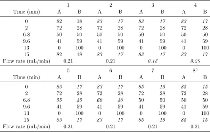
Table 2.1: Gradient program and flow rate for the eight experiments. Shown are the

proportion of 0.1% phosphoric acid aqueous solution (A) and acetonitrile (B) in the

mobile phase and the timings of the changing of relative proportions along with the flow rate of the mobile phase. The italicized values indicate the altered parameters in comparison to those in condition 1.

1 2 3 4

Time (min) A B A B A B A B

0 82 18 83 17 83 17 83 17

2 72 28 72 28 72 28 72 28

6.8 50 50 50 50 50 50 50 50

9.6 41 59 41 59 41 59 41 59

13 0 100 0 100 0 100 0 100

15 82 18 83 17 83 17 83 17

Flow rate (mL/min) 0.21 0.21 0.18 0.20

5 6 7 8a

Time (min) A B A B A B A B

0 83 17 83 17 85 15 85 15

2 72 28 72 28 72 28 72 28

6.8 55 45 60 40 50 50 50 50

9.6 41 59 41 59 41 59 41 59

13 0 100 0 100 0 100 0 100

15 83 17 83 17 85 15 85 15

Flow rate (mL/min) 0.21 0.21 0.21 0.21

a_{Time at which last two concentration changes occur at 12 and 14 minutes, respectively}

For each of the eight experimental conditions, we analyze three samples of rhubarb via

HPLC. The conditions are constructed by varying the gradient program and flow rate

as described in Table 2.1. Each sample is run using the ACQUITY BEH C18column

held at 30 degrees Celsius. The wavelength of the UV detector is set at 260 nm. The

(25)

The observed total retention times ranged from 14.0021 to 16.0025 minutes. The

observed vectors for conditions 1–8 were of respective lengths {19200, 18000, 18000,

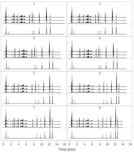
18000, 18000, 18000, 18000, 16800}. Figure 2.1 displays the chromatograms for the

24 samples. To illustrate the ability to identify compounds across different conditions

using the fingerprint of a set of known compounds under one single condition, we also

analyzed a mixture of seven compounds known to be in rhubarb under condition 1

(Ye et al., 2007) and the resulting chromatogram is displayed in Figure 2.1. The 7

known compounds are (1) gallic acid, (2) catechin, (3) aloe-emodin, (4) rhein, (5)

emodin, (6) chrysophanol, and (7) physcion.

2.3. Model

Let yijk be observation k from chromatogram j in experimental condition i at time

pointtijk, where we assume without loss of generality thattijk ∈[0,1],i= 1,2, . . . , n,

j = 1,2, . . . , m, k = 1,2, . . . , Li. Our model is

yijk =f(τijk) +eijk, τijk =g(tijk,bi) (2.1)

wheref is an unknown spiky function,τijk is the warped time relating totijkvia some

smooth monotonic function g, indexed by unknown condition-level parameter vector

bi, andeij = (eij1, . . . , eijLi)

T _{is the vector of measurment errors for chromatogram}_j

with mean 0 and covariance matrix σ2_V

i(θ), where θ is a vector of unknown

param-eters and σ2 _{is an unknown scale parameter.} _V

i depends on ithrough its dimension.

In this chapter we assume equal number of experiments per condition and each

ex-periment within a condition are observed on the same time vector, however these

assumptions can be relaxed.

(26)

1 2 3 4 5 6 7 1 1

2 3 4

5 6 7 1 2 3 4 5 6 7 2 1

2 3 4

5 6 7 1 2 3 4 5 6 7 3 1

2 3 4

5 6 7 1 2 3 4 5 6 7 4 1

2 3 4

5 6 7 1 2 3 4 5 6 7 5 1

2 3 4

5 6 7 1 2 3 4 5 6 7 6 1

2 3 4

5 6 7 1 2 3 4 5 6 7 7

0 2 4 6 8 10 12 14 16

1

2 3 4

5 6 7 1 2 3 4 5 6 7 8

0 2 4 6 8 10 12 14 16

1

2 3 4

5 6 7

Time (min)

(27)

basis, that is f(τijk) =Pp_s₌₁xs(τijk)βs, where xs(τijk) is the sth spline wavelet basis

function evaluated atτijk andβsis the corresponding unknown basis function

param-eter. In wavelet bases, thexsestimate oscillations in the observed signal at particular

dyadic scales and integer translates for different s. Battle-Lemari´e spline wavelets

possess a number of attractive properties such as orthogonality, regularity, vanishing

moments, symmetry, and a closed-form expression (Daubechies, 1992; Unser, 1997).

Some common examples of parametric models for the warping functions include:

a linear combination of polynomial functions g(tijk,bi) = PQ_q₌₀bqtq_ijk. By setting

bq = 0 for q > 1 we get the location and scale functions as in shape-invariant and

self-modeling regression models (Lawton et al., 1972). A more flexible example is a

linear combination of B-splines: g(tijk,bi) = Bq,r(tijk)bi,whereBq,r(tijk) is the 1×Q

design matrix of B-spline basis functions of orderq and knot sequencer evaluated at

tijk (Brumback and Lindstrom, 2004). We focus on estimation using B-splines with

a uniform knot sequence in the current chapter.

The time warping functions are constrained to be monotonic so that no time point

in the original scale is mapped to more than one time point in the warped scale.

B-splines are a convenient choice of basis as imposing monotonicity in the warping

functions can be accomplished by imposing monotonicity in the B-spline coefficients

(Schumaker, 2007, chap. 4.9). Numerically, we can either invoke inequality

con-straints for eachior reparametrize the sequential increments of the coefficients by an

exponential transformation resulting in a sequence of increasing B-spline coefficients.

That is, for condition i, letting bil be the lth parameter for condition i, we set

(28)

where δij ∈ (−∞,∞), j = 2, . . . , Q. As with most wavelet bases, a boundary

con-straint must also be placed on the wavelet basis, such as periodicity or symmetry.

As such, a further constraint must be placed on the B-spline coefficients to maintain

identifiability of the warped time vector. For example, assuming periodic wavelets,

we can constrain bi1 to be in [−0.5,0.5] to ensure identifiability. This can be

accom-plished by letting bi1 = exp(δi1)/(1 + exp(δi1))−0.5 where δi1 ∈ (−∞,∞). While

there is a monotonic constraint among the B-spline coefficients, we do not need to

consider explicit constraints in estimating δi1,· · · , δiQ.

To set a particular experimental condition as the reference time scale, we set the

warping function parameters of one condition to correspond to the 45 degree line,

which denotes no warping. For example, for cubic B-splines with k uniform knots,

the coefficients for the reference condition are equal to {0,1/(3k−3), . . . ,3z/(3k−

3), . . . ,(3k−4)/(3k−3),1}, for z = 1, . . . k−2. Without loss of generality, we select

condition 1 as the reference condition.

Thus (2.1) can be expressed as:

yijk = p

X

s=1

xs{τijk}βs+eijk, τijk =Bq,r(tijk)bi (2.2)

As we wish to restrict the number of parameters to be less than the number of data

points per curve, p should be less than min(Li)−Q(n−1). Thus the total number

(29)

2.4. Estimation

Let yij = (yij1, . . . , yijni)

T_, _t

ij = (tij1, . . . , tijni)

T_{, and} _b

i = (bTi1, . . . ,bim)T. The

penalized weighted least squares criterion is:

1 2σ2

n X i=1 m X j=1

yij − p

X

s=1

xs{g(tij,bi)}βs

!T

V_i−1(θ) yij − p

X

s=1

xs{g(tij,bi)}βq

! +λ p X j=1 ˆ

wj(|βj|)

(2.3)

where ˆwj are data-driven weights, andλis a tuning parameter for the Adaptive Lasso

penalty which controls the amount of shrinkage. We use ˆwj = |βˆjNLS|−1 where ˆβjNLS

is the unpenalized, nonlinear weighted least squares estimator of βj as it is a root-n

consistent estimator of ˆβj (Jennrich, 1969).

Letting b = (bT

2, . . . ,bTn)T, computation can be greatly simplified by setting λ

∗ ₌

σ2_λ_{, and noting that for fixed} _b _{= ˆ}_b _and _θ _{= ˆ}_θ_{, solving (2.3) for} _β _{simplifies to a}

penalized least squares problem with the Adaptive Lasso penalty:

ˆ

β= arg min

β   

y_ij∗ −

p

X

s=1

x∗_s{g(tij,bˆi)}βs

2 2 +λ∗ p X j=1 ˆ

wj(|βj|)

  

(2.4)

where y∗_ij = V_i−1/2( ˆθ)yij and xs(·)∗ = V

−1/2

i ( ˆθ)sxs(·) where V

−1/2

i (θ)s is the sth

row of V_i−1/2(θ). Minimizing (2.4) can be accomplished using standard algorithms

for `1-penalized regression (Zou, 2006). For fixed β = ˆβ and θ = ˆθ, using the

reparameterization of bi described in the previous section, solving (2.3) for b is

(30)

δ = (δ21, . . . , δ2Q, . . . , δn1, . . . , δnQ)T:

ˆ

δ = arg min

δ n X i=1 m X j=1

y∗_ij −

p

X

s=1

x∗_s(g{tij,δi)}βˆs

2 2 (2.5)

Similarly, for fixed β = ˆβ and b = ˆb, solving (2.3) for θ is also an unpenalized

nonlinear least squares problem:

ˆ

θ = arg min

θ n X i=1 m X j=1

V_i−1/2(θ) yij − p

X

s=1

xs(g{tij,bˆi)}βˆs

! 2 2 (2.6)

Hence we propose the following iterative back-fitting algorithm to estimateβ,b, and

θ:

At iteration k:

1. Fix the b and θ at their estimates from iteration (k−1), denoted b(k−1) _and

θ(k−1)_{. Solve (2.4) for} _β_{, obtaining ˆ}_β(k−1)_.

2. Fixβ at ˆβ(k−1) from step 1 and θ atθ(k−1). Solve (2.5) for δ, obtaining ˆδ(k−1)

and ˆb(k−1).

3. Fixβ at ˆβ(k−1) _and _b_{at ˆ}_b(k−1) _{from steps 1 and 2, respectively. Solve (2.6) for}

θ, obtaining ˆθ(k−1)_.

Iterate steps 1–3 until convergence. At convergence, estimate σ2 _via

ˆ

σ2 = 1

mPn

i=1Li n X i=1 m X j=1

V_i−1/2( ˆθ) yij − p

X

s=1

xs{g(tij,bˆi)}βˆs

! 2 2 (2.7)

The algorithm as a whole minimizes the unified criterion, (2.3), and by using line

(31)

algorithm (Tseng, 2001).

Convergence of the back-fitting algorithm depends on good initial estimates.

Specif-ically, the algorithm requires good initial estimates of the warping function

parame-ters. One method for obtaining initial estimates is to set λ = 0 and solve (2.3). In

this situation, (2.3) is an unpenalized nonlinear least squares problem. As standard

nonlinear least squares procedures are iterative, initial estimates of the warping

func-tion parameters are necessary for this step, as well. These can be obtained by first

estimating the warping functions via dynamic time warping (Kassidas et al., 1998;

Giorgino, 2009) and then modeling the estimated warping functions using monotonic

B-splines.

It is important to note that since the bi are updated at each iteration, the wavelet

basis design matrix also changes at each iteration. The adaptive weights, |βˆNLS_|−1_,

are calculated at the initial estimation step using the unpenalized estimates and are

kept constant throughout the estimation procedure.

The estimates obtained from (2.3) depend on the particular value of the tuning

parameter, λ, as the proposed back-fitting algorithm is for a fixed λ. Numerous

techniques to choose the optimal value of λ exist with varying degrees of properties.

In penalized least squares problems with the smoothly clipped absolute deviation

(Fan and Li, 2001) chosen as the penalty, it has been shown that BIC consistently

chooses the correct model (Wang et al., 2007). This results follows when using the

Adaptive Lasso. We use the BIC to choose the optimal value of λ.

Our proposed method does not require normality. In practice, when applying our

procedure to chromatographic data, we have found that the tails of the distribution of

(32)

the Lasso to fat-tailed errors has been studied previously. Finite sample performance

is affected by fat tails, however Fan et al. (2013) showed that Lasso estimates retain

sign consistency if the signal is large enough. Bunea and Gupta (2010) and Sang

and Sun (2012) consider Lasso and SCAD estimates under correlated data, including

auto-regressive errors, and show that their asymptotic properties are still valid. As

chromatograms exhibit a large signal-to-noise ratio and contain thousands of data

points, heavy-tailed errors should not pose a problem in practice.

The model estimates possess attractive sampling properties. As in Zou (2006), we

assume, without loss of generality, that there is ap0 < p such that|βk|>0 fork ≤p0

and βk = 0 for p0 < k ≤ p. Thus the true active set of β, A, is {1,2, . . . p0}. Let

ˆ

An = {j : ˆβj = 06 } be the estimated active set of β, where ˆβj is the estimate of βj

from the adaptive lasso criterion.

Theorem 1. Let ψ = (θT,bT,βT)T and ψA = (θT,bT,βTA)T. Under the regularity

conditions described in Fan and Li (2001); Zhang and Lu (2007); Bunea and Gupta

(2010), the estimates obtained by minimizing (2.3) satisfy the following:

1. limn→∞P( ˆAn =A) = 1.

2. √n( ˆψA−ψA)→ N(0, σ2C−1).

where _n1 P

if(ψA)V

−1₍_θ₎_f₍_ψ

A)T →C.

The proof of Theorem 1 follows very closely to the corresponding proofs in Fan and

Li (2001); Zhang and Lu (2007); Bunea and Gupta (2010), so it is omitted. Theorem

1 shows that the adaptive lasso estimators obtained from (2.3) are variable selection

consistent, root-n consistent, and asymptotically normal. Thus, the estimators

pos-sess the oracle property (Donoho and Johnstone, 1994). The root-n consistency is

(33)

parameter coefficients. The asymptotic normality of the estimates enables the

con-struction of asymptotic confidence intervals for the estimated fingerprint and warping

functions which reflect the combined variability in estimatingβ,b, and θjointly. For

example, by taking a Taylor expansion off about the true value ofψ, we estimate the

approximate asymptotic variance for the estimated fingerprint as ˆσ2_s_{( ˆ}_ψ₎_C−1_s_{( ˆ}_ψ₎T_,

where s( ˆψ) = ∂f( ˆψ)/∂ψ.

2.5. Application to Data Example

We applied (2.2) to the rhubarb chromatographic dataset described in Section 2.2.

For computational efficiency, we subsampled the data such that the data vectors

for the eight conditions were of respective lengths {2743, 2572, 2572, 2572, 2572,

2572, 2572, 2400}. The observed time vectors were mapped to [0,1] by setting the

maximum observed time, 16.0025 min., to 1.

Spline wavelets can be evaluated at any arbitrary time point, however the

compu-tation involves nested summations of many terms, so for compucompu-tational speed, we

computed the design matrix at arbitrary time points using the following procedure:

a reference design matrix is evaluated on a grid of 217 _{time points in [0}_,_{1]. Design}

points are computed via a table-look-up and for time values not in the reference design

matrix, interpolation between adjacent points is used. We chose the finest wavelet

scale to be 10, resulting in 2048 basis functions where the 2i,2i+ 1, . . . ,(2i+1−1)th

functions correspond to the wavelet basis functions at scalei. The finest level wavelet

scale is chosen based on the data so that the resolution is fine enough to capture the

narrowest spikes. We assume periodic boundary conditions for convenience.

To model the warping functions, we used monotonic cubic B-splines with 14

(34)

appears to work well for a moderate amount of warping. We assume a first-order

auto-regressive correlation structure, thusθ is a scalar, denotedθ, and represents the

correlation between points one unit of time apart.

The algorithm was written in MATLAB and run on an Intel Xeon CPU E7-4860.

For each value of λ, the algorithm converged in less than five outer iterations, and

finished, on average, in 10 minutes. The adaptive lasso parameterλ, found using BIC

and a golden search algorithm, was 0.489. The estimated variance of the measurement

error was 1.24×10−3 and the estimate for θ was 0.698.

0 2 4 6 8 10 12 14 16

0.0

0.2

0.4

0.6

0.8

1

2

3

4 5

6

7

Time (min)

Intensity (A

U)

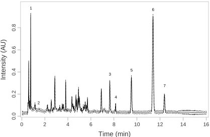
Figure 2.2: Population averaged fingerprint (solid) from the estimates along with 95% confidence bands (dashed). Identified compounds are denoted: (1) gallic acid, (2) catechin, (3) aloe-emodin, (4) rhein, (5) emodin, (6) chrysophanol, and (7) physcion.

The population averaged estimate of the standardized chromatographic fingerprint

(35)

scale corresponds to the real time scale under condition 1. The population-averaged

curve captures the shape of the individual chromatograms quite well, resulted from

a good alignment across conditions. As the known compounds were analyzed under

condition 1, spike locations between the reference chromatogram and the estimated

fingerprint can be compared. The seven spikes that correspond to the known

com-pounds are labeled in Figure 2.2.

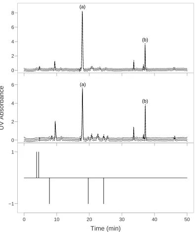
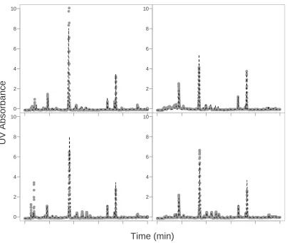
To identify the seven known compounds in other conditions, we use the inverse

es-timated warping functions to warp the reference chromatogram in condition 1 to

the time scale of each other condition. The estimated reference chromatograms are

displayed in Figure 2.1 along with the raw data. By comparing with the estimated

ref-erence chromatograms, the seven known compounds are identified in each condition.

These also show that we are able to estimate each warping function accurately.

The final estimate of the fingerprint shape contained 427 nonzero wavelet coefficients,

while the remaining 1621 were shrunk to 0. This highlights the sparse nature of the

fingerprint shape as a little more than 79% of the wavelet basis functions are

irrele-vant. The confidence intervals for the fingerprint can be used to determine whether

a spike is artificial or real based on whether the corresponding confidence interval

contains 0 or not. For example, the amplitude of the spike corresponding to catechin

is small however the confidence interval at the peak of the spike is [0.014,0.044],

suggesting it is present in rhubarb, which coincides with previous research (Ye et al.,

2007).

The groups of tightly-packed spikes located between 4 and 6 minutes in the fingerprint

can either correspond to single compounds or multiple compounds which were not

well separated in the HPLC column. If we wished to identify the compounds in this

(36)

that these particular compounds are better separated and travel through the column

at more distinct velocities. This would result in more spacing among spikes in this

region of the chromatograms.

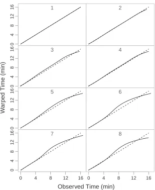
Figure 2.3 displays the estimated warping function for each of the eight conditions.

Confidence intervals were computed for the warping functions however due to the

low variance of the B-spline coefficients (Var(bi) ∼ O(10−4)), the bands are visually

indistinguishable from the estimated warping functions. The low order of variance is

due to the large effective sample size.

The estimated warping functions represent the distortion in retention time of

condi-tions 2–8 in comparison to condition 1. The relative proporcondi-tions of phosphoric acid

and acetonitrile differs by only 1% at time 0 between conditions 1 and 2, and this

difference caused little to no warping, as evidenced by the estimated warping

func-tion of condifunc-tion 2. Conversely, a 3% change, as in condifunc-tion 7, results in substantial

warping after minute 4. The estimated warping functions for conditions 3 and 4 in

comparison to those for conditions 5–8 suggest that flow rate does not have quite as

large of an impact on retention time as the composition of the mobile phase.

2.6. Simulation

A vast number of mathematical functions have been proposed to simulate

chromato-graphic data (Di Marco and Bombi, 2001). One such example is the Laplace

distribu-tion funcdistribu-tion. We simulated the true fingerprint shape by overlaying a fixed number

of spikes, where each spike was generated via f(t) =aexp(−|t−c|/b)/(2b) where a

controls the amplitude of the spike,cthe location of the maximum of the spike, andb

is a scale parameter, affecting the width and tails of the spike. We used twelve spikes

(37)

1

0

4

8

12

16 2

3

0

4

8

12

16 4

5

0

4

8

12

16 6

7

0 4 8 12 16

0

4

8

12

16 8

0 4 8 12 16

Observed Time (min)

W

ar

ped Time (min)

Figure 2.3: The estimated warping functions (solid) along with the 45 degree line denoting no warping for each condition (dashed).

were generated from a N(20,25) distribution and the scale parameters were sampled

with replacement from the set {0.45,0.50, . . . ,0.75}.

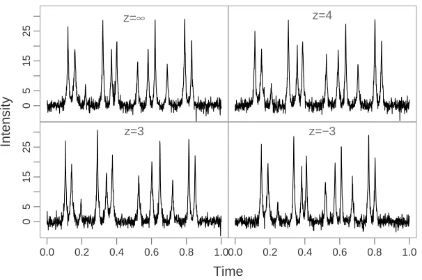
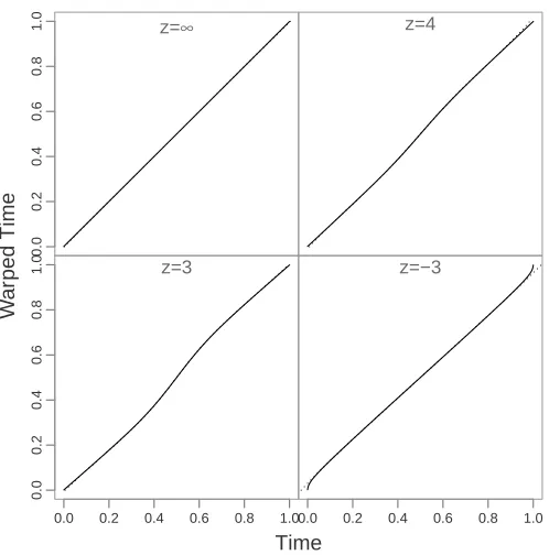
To simulate time warping similar to those seen in the rhubarb data, the time warping

functions were generated by the following logistic function, g(t) = [1 + exp(−14t+

7))]−1. The point-wise mean betweeng(t) and the 45 degree line, denoting no warping,

can be iteratively calculated to generate warping functions with similar shape, but

(38)

the function and the 45 degree line, then the warping function deviates less from the

45 degree line as z increases and converges to the 45 degree line as z → ∞. The

inverse logistic function was used to generate one warping function with a mirrored

shape to the rest. For notational brevity, a negative value ofzcorresponds to iterated

averaging the 45 degree line with the inverse logistic function z times.

A set of four warping functions were generated using z ={∞,4,3,−3}, representing

four different experimental conditions, and the warping functions were estimated

us-ing three, four, and five uniform knots. For each condition we generated 4 fus-ingerprints

sampled on 1000 equispaced time points in [0,1]. We added t-distributed noise, with

9 degrees of freedom, to each curve. The t-distribution was used as it has longer tails

than the normal distribution. Figure 2.4 displays an example of a noisy fingerprint

from each condition.

For comparison, we also fit a two-step model where the first step used dynamic time

warping to align the curves and the second applied a wavelet thresholding to the

aligned curves and averaged across the curves to obtain the population averaged

fingerprint. The dynamic time warping step was accomplished using the ‘dtw’

pack-age in R (Giorgino, 2009) and the wavelet thresholding was performed using the

‘wavethresh’ package in R (Nason, 2008). We simulated 100 datasets and performed

the four methods on each set.

The proposed model was fit using 29 = 512 cubic Battle-Lemari´e spline wavelet basis

functions to model the shape and cubic B-splines to model the warping function.

For each value of λ, our algorithm converged in less than five outer iterations and

finished, on average, in 40 seconds. We also used 512 cubic Battle-Lemari´e spline

wavelets for the two-step method and the Bayesian approach of Abramovich et al.

(39)

z=∞

0

5

15

25

z=4

z=3

0.0 0.2 0.4 0.6 0.8 1.0

0

5

15

25

z=−3

0.0 0.2 0.4 0.6 0.8 1.0

Time

Intensity

Figure 2.4: Simulated warped curves with 12 peaks and additive t-distributed noise. The curve was generated using the Laplace distribution function and the warping functions were generated by logistic and inverse-logistic functions.

To assess the fits, boxplots of the mean squared error (MSE) between the true and

estimated fingerprints were used, which are displayed in Figure 2.5. First, the

pro-posed 4- and 5-knot models performed the best. The 3-knot model performed the

worst of the four methods. This is due to the fact that three knots does not provide

enough flexibility in capturing the shape of the warping functions. The boxplots

suggest that by estimating the warping function using B-splines with at least four

uniform knots, the degree of the warping does not appear to affect the MSE in any

substantial way. The two-step approach does not perform as well as the proposed

4-and 5-knot models, though it outperforms the 3-knot model.

Figure 2.6 displays the mean of the estimated warping functions across all 100

sim-ulations for the proposed 4-knot model overlaid on the true warping functions. The

proposed model with four knots estimates the true warping functions well except at

the ends of the tails, where there is slight deviation. Though we only consider

(40)

function, our simulation shows that a large amount of flexibility is not required for

quality performance of the modeling procedure.

SSNM3 SSNM4 SSNM5 2−step

0.2 0.4 0.6 0.8

Method

Mean Squared Error

Figure 2.5: Boxplots of the mean square error of the estimated fingerprints for the proposed procedure using 3-, 4-, and 5-knots and the two-step procedure using dy-namic time warping and wavelet thresholding.

2.7. Discussion

We have proposed a sparse semiparametric nonlinear model for the registration of

chromatographic data and establishment of a standardized fingerprint. The common

shape of the chromatograms is modeled via data-driven basis expansion. Curve

reg-istration is accomplished by parametric modeling of the time warping functions. As

chromatograms are sparsely-structured curves, we impose the adaptive lasso penalty

on the common shape basis function parameters to induce sparsity in the estimated

fingerprint. A unified penalized weighted least squares criterion is minimized to

(41)

z=∞

0.0

0.2

0.4

0.6

0.8

1.0 z=4

z=3

0.0 0.2 0.4 0.6 0.8 1.0

0.0

0.2

0.4

0.6

0.8

1.0 z=−3

0.0 0.2 0.4 0.6 0.8 1.0

Time

W

ar

ped Time

Figure 2.6: True (solid) and mean of 100 estimated warping functions (dashed) using 4 uniform knots.

shape, and estimate the model parameters. From the penalized criterion naturally

arises a back-fitting algorithm which is equivalent to a blockwise coordinate descent

algorithm. The unified criterion results in a unique solution and allows the study of

asymptotic properties, as opposed to two-step methods which can guarantee neither.

Our resulting estimators possess the oracle property.

We applied our model to a chromatographic dataset of the TCHM, rhubarb. Our

model was effective in establishing a standardized fingerprint of rhubarb based on

chromatograms arising from different experimental conditions. A sample of known

compounds was analyzed under a single condition to identify compounds in the

fin-gerprint. We demonstrated that known compounds need only be analyzed under

a single condition, substantially decreasing both time and cost of chromatographic

(42)

We use BIC to select the tuning parameterλhowever other tuning parameter selection

techniques such as AIC, GCV, and Stein’s unbiased risk exist, and in our simulations,

performed similarly. We have focused the discussion on modeling the common shape

using a linear combination of wavelet basis function and the warping functions using

monotonic B-splines, however the proposed model can be easily extended to include

multiple population average curves or in the situation that the observations relate to

(43)

CHAPTER 3 Semiparametric Nonlinear Mixed Effects Models for

Sparsely-Structured Functional Data

3.1. Introduction

Functional data arise in numerous applications in pharmacological, environmental,

and biomedical research including chromatographic, weather pattern, biomarker, and

growth hormone studies. The cornerstone of functional data analyses is viewing the

observed data as samples of unknown functions and modeling the data as curves. A

common objective in functional data analyses is aligning data curves and estimating

and comparing their structures, such as spikes.

Our research is motivated by a study of the chemical composition of the medicinal

herb, Andrographis paniculata. Medicinal herbs have been used for the treatment

of a number of medical ailments for thousands of years (Duke, 2002; Chao and Lin,

2010). As the exact chemical composition of an herb differs based on its particular

species and origin, properties of the seed and field used to grow the herbs, and the

particular processes used in the growing, harvesting, and storage of the herbs (Leung

and Cheng, 2008), tools and methodologies for composition determination and the

identification of compounds not shared between, say, production sites are vital for

the quality control of herbal medications.

High Performance Liquid Chromatography (HPLC), which is a set of techniques to

separate compounds of biological mixtures, has played a large role in medicinal herb

(44)

characterized by a number of spikes, where each spike corresponds to a particular

compound in the herb. Since the location of spikes in the curve can be used to identify

the compounds and the chemical composition is unique to an herb, chromatograms

provide a fingerprint of an herb. Consider Figure 3.1 which displays chromatograms

of samples of Andrographis paniculata collected from two types of production sites:

five sites which comply with Good Agricultural Practices (GAP) and five pharmacies

whose GAP compliance unknown and analyzed using HPLC. The objective of the

study is to compare the compositions of samples between the two groups, GAP

and pharmacy, or market sites, and identify compounds present in one group of

herbs but not the other. The presence of any discordant compounds will suggest

deficiencies in the production processes of the market sites. Further details regarding

GAP are described in Section 3.4. Through HPLC, comparing compositions between

GAP and market herbs amounts to comparing their group-averaged chromatographic

fingerprints.

However, a number of characteristics of chromatograms evident in Figure 3.1

im-pede the direct establishment of chromatographic fingerprints and their comparison.

First, spiky curves, such as chromatograms, are not well estimated by parametric

functions. This common issue in functional data analyses can be addressed by

ex-panding the curve into some basis system such as splines or wavelets (Ramsay and

Silverman, 2005). Second, due to differing experimental and environmental

condi-tions, the timings of spikes in chromatograms often vary across experiments. The

site-level transformations of the curves induce misalignment of spikes and prevent

the establishment and comparison of group-averaged curves. Curve registration is a

set of methodologies in which features of interest are aligned by warping the

(45)

0 10 20 30 40 50 0 10 20 30 40 50

Time (min)

(46)

is accomplished by modeling the unknown, monotonic time warping function within

the basis expansion of the fingerprint shapes, as in shape-invariant and self-modeling

regression models (SEMOR) models (e.g. Lawton et al., 1972; Ke and Wang, 2001;

Brumback and Lindstrom, 2004). Since there are a large number of production sites

under study and the number of parameters in SEMOR models increases with the

number of sites. Thus, along with the fact that we wish to compare group-averaged

curves while taking into account the correct sources of variability, warping function

parameters should be modeled as random (Ke and Wang, 2001; Guo, 2002). Thus,

curve registration offers a flexible, nonlinear framework to align and estimate spikes.

Finally, thousands of data points are collected per chromatogram but the curves

exhibit only a small number of sharp, narrow spikes. The large sections of the curves

between spikes are flat and do not contain meaningful signal. Due to their sparse

nature, estimating curves via basis expansion results in the irrelevancy of a large

number of basis functions as they correspond to the flat section and are merely

estimating noise. As their true coefficient value is 0, these superfluous variables

need to be excluded to avoid overfitting. As such, identifying, or selecting, important

functions while leaving out irrelevant functions is a necessary component to modeling

sparsely-structured functional data. As we wish to select the functions whose true

coefficient values are not equal to zero, this falls within the model selection framework.

There exist numerous methods for the analysis of chromatographic data. For

exam-ple, Morris et al. (2008) model mass spectrometry data, which is similar in nature to

chromatographic data, using a wavelet-based functional mixed effects model

(Mor-ris and Carroll, 2006). The model is an extension of the functional mixed effects

models of Guo (2002) to the sparsely-structured setting and can accommodate a

(47)

levels of nested structures. However the models of Guo (2002); Morris and

Car-roll (2006); Morris et al. (2008) are linear in the mixed effects and so data which

exhibit subject-specific transformations of the common shape functions cannot be

adequately modeled within these frameworks. Much like most current methods for

chromatographic data, Morris et al. (2008) circumvents this issue by aligning curves

in a pre-processing step. By aligning individual curves and estimating mean curves

in separate steps, the variability in the alignment step is ignored in the second step.

Thus variance estimates, which do not account for both phase and measurement error

variability, will be incorrect and valid statistical inference cannot be drawn. A model

which allows for the mixed effects to enter into the model nonlinearly is needed.

Ke and Wang (2001) proposed a general class of semiparameteric nonlinear mixed

effects models (SNMM), which includes extensions of nonlinear mixed effects and

SEMOR models. SNMMs can handle numerous curve shapes encountered in practice

and allow for nonlinearity in the mixed effects specification. Ke and Wang (2001)

pro-pose estimating the mean functions nonparametrically with parametrically-specified

covariates using a double-penalized likelihood criterion. They propose an iterative

back-fitting estimation algorithm where the first step estimates the shape function

via smoothing splines and the second estimates fixed and random effects and variance

components via a nonlinear mixed effects model through linearization of the

likeli-hood about the random effects. However, the second step of the estimation algorithm

in Ke and Wang (2001) ignores the fact that the random effects are allowed to enter

into the shape functions (Lin and Zhang, 2001; Elmi et al., 2011). As shown in Lin

and Zhang (2001), their estimation procedure is equivalent to a two-step procedure

in which each step fits a separate mixed effects model. As the two mixed effects

Nonlinear Structural Functional Models

University of Pennsylvania

ScholarlyCommons

Nonlinear Structural Functional Models

Michael Ryan Wierzbicki

Nonlinear Structural Functional Models

ACKNOWLEDGMENT

ABSTRACT

TABLE OF CONTENTS

LIST OF TABLES

LIST OF ILLUSTRATIONS

CHAPTER 1

Introduction

CHAPTER 2

Sparse Semiparametric Nonlinear Model with Application

to Chromatographic Fingerprints

2.1. Introduction

2.2. Data

2.3. Model

2.4. Estimation

2.5. Application to Data Example

Time (min)

Intensity (A

U)

2.6. Simulation

2.7. Discussion

CHAPTER 3

Semiparametric Nonlinear Mixed Effects Models for

Sparsely-Structured Functional Data

3.1. Introduction