Overlapping sea level time series measured using different technologies: an example from the REDMAR Spanish network

(1)

Nat. Hazards Earth Syst. Sci., 14, 589–610, 2014 www.nat-hazards-earth-syst-sci.net/14/589/2014/ doi:10.5194/nhess-14-589-2014

Natural Hazards

and Earth System

Sciences

Open Access

Overlapping sea level time series measured using different

technologies: an example from the REDMAR Spanish network

B. Pérez1, A. Payo2,*, D. López2, P. L. Woodworth3, and E. Alvarez Fanjul1 1_{Puertos del Estado, Madrid, Spain}

2_{SIDMAR Bernhard Pack S.L., Benissa, Alicante, Spain} 3_{National Oceanography Centre, Liverpool, UK}

*_{now at: Environmental Change Institute, University of Oxford, UK}

Correspondence to: B. Pérez ([email protected])

Received: 19 December 2012 – Published in Nat. Hazards Earth Syst. Sci. Discuss.: – Revised: 26 September 2013 – Accepted: 13 October 2013 – Published: 13 March 2014

Abstract. This paper addresses the problems of overlapping sea level time series measured using different technologies and sometimes from different locations inside a harbour. The renovation of the Spanish REDMAR (RED de MAReó-grafos) sea level network is taken here as an example of the difficulties encountered: up to seventeen old tide gauge sta-tions have been replaced by radar tide gauges all around the Spanish coast, in order to fulfil the new international require-ments on tsunami detection. Overlapping periods between old and new stations have allowed the comparison of records in different frequency ranges and the determination of the im-pact of this change of instrumentation on the long-term sea level products such as tides, surges and mean sea levels. The differences encountered are generally within the values ex-pected, taking into account the characteristics of the different sensors, the different sampling strategies and sometimes the different locations inside the harbours. However, our analy-sis has also revealed in some cases the presence of significant scale errors that, overlapping with datum differences and un-certainties, as well as with hardware problems in many new radar gauges, may hinder the generation of coherent and con-tinuous sea level time series. Comparisons with nearby sta-tions have been combined with comparisons with altimetry time series close to each station in order to better determine the sources of error and to guarantee the precise relationships between the sea level time series from the old and the new tide gauges.

1 Introduction

(2)

590 B. Pérez et al.: Overlapping sea level time series measured using different technologies

28 Fig. 1.REDMAR sea level network in 2012: 35 MIROS stations and 2 AANDERAA pressure 1

sensors in the Canary Islands. Detailed maps show by white circles the positions of the older 2

tide gauges (SRD or AANDERAA) that were renovated or upgraded with MIROS radar 3

gauges. The remaining points shown by red circles are completely new stations established 4

between 2006 and 2012. The attached table includes the accuracy and resolution of each of 5

the sensors, claimed by the manufacturers, assuming a 5 m tidal range and 1-min averages. 6

7

SRD AANDERAA MIROS

Accuracy (mm) 2.5 10 1

Resolution (mm) 10 5 1

8 9 10 11 12

Fig. 1. REDMAR sea level network in 2012: 35 MIROS stations and 2 AANDERAA pressure sensors in the Canary Islands. Detailed maps

show by solid white circles the positions of the older tide gauges (SRD or AANDERAA) that were renovated or upgraded with MIROS radar gauges. The remaining points shown by solid red circles are completely new stations established between 2006 and 2012. The attached table includes the accuracy and resolution of each of the sensors, claimed by the manufacturers, assuming a 5 m tidal range and 1 min averages.

In 2002 a pilot station was established in Vilagarcía har-bour, on the northwest coast of Spain, for testing up to eight different acoustic, radar and pressure sensors (Martín Míguez et al., 2005). After more than one year of simultaneous mea-surements, the MIROS (MIcrowave Remote sensor for the Ocean Surface) FMCW (frequency modulated continuous wave) radar sensor was selected based on the following cri-teria:

– High-precision of the individual measurements and se-lectable data sampling (1 min or less);

– 2 Hz original raw data sampling that allowed wind wave or agitation (short waves inside the bour) parameters to be estimated (needed in some har-bours);

– Good performance and stability of the datum ; – Good communication with the manufacturer for

im-plementation of additional requirements of Puertos del

Estado for the REDMAR network: data formats, GPS (Global Positioning System) time control, etc.

(3)

B. Pérez et al.: Overlapping sea level time series measured using different technologies 591

and Melilla (North Africa) (Fig. 1). Most of the new stations are particularly important for tsunami monitoring purposes in the European/Mediterranean region, although their instal-lation is meant to satisfy also all other possible applications. Monthly mean sea levels of the REDMAR network are provided annually to the Permanent Service for Mean Sea Level (PSMSL, www.psmsl.org) and the data are used by sci-entists all around the world. For this reason one of the main concerns during this process of renovation was to guarantee the continuity of the longer time series of sea level. Taking this into account, most of the new stations overlapped dur-ing at least one year with the old stations (solid white circles in Fig. 1), following the recommendation of the Global Sea Level Observing System (IOC, 2006), except at Coruña sta-tion, where a sudden malfunction of the SRD sensor with no spare parts available reduced the overlapping period to just 10 months, and at Valencia, where harbour development forced the dismantling of the old station after just 4 months.

The process of comparison has been performed for 5 min, hourly, daily and monthly values, in order to account for the different sea level processes. Comparisons also include the main harmonic constants and the residual component (ob-servations – tide). Some of the new tide gauges are at ex-actly the same location as the old tide gauge, making datum connection easier; in these cases the expected differences at all frequencies should be small. However, when the new tide gauge has been installed at another location in the harbour with different agitation/high frequency variability, only the lower frequencies of sea level are expected to be coherent with the old station, and a high precision levelling is needed to connect both tide gauges to the same datum.

As the adequacy of the MIROS radar sensor was as-sessed in previous experiments, such as the one in Vilagarcía (Martín Míguez et al., 2005), the objective of this study is fo-cused on the scientific impact of the technological renovation of the network, assessed by identifying the differences in the sea level signals and their influence on the different products such as the long-term time series provided to the PSMSL. Decisions about correcting the data, or providing informa-tion as metadata if necessary, will result from this study. It is not intended here to make a comprehensive analysis of all possible sources of error at each station, but special emphasis has been placed on the datum connection between stations, the scale errors that generate a bias in the data and the influ-ence of a delamination problem detected in the radar sensors, as these may affect the long-term trends in mean sea levels. For this, use of altimetry data has allowed a better determina-tion of the impact of the network renovadetermina-tion in the monthly means. A detailed review of these differences should also be taken into account for extreme analysis studies (not included in this paper), historical evolution of tides and tidal ranges, etc.

The paper is structured as follows: the second section presents a review of the main sources of error, general or specific to REDMAR, that can result in differences between two simultaneous tide gauge data sets from the same har-bour; the third section will describe the data employed and the methodology for data comparison during REDMAR ren-ovation; and the fourth section will present the results and discussion of this comparison exercise as well as the impact of the network renovation on the main sea level products.

2 Sources of error and differences between two tide gauges

There are many technical and environmental/oceanographic factors that can result in differences between tide gauge data sets in a comparison exercise (Lennon, 1967; Shih and Porter, 1981; Lentz, 1993): geophysical peculiarities of the tide gauge location such as harbour resonances, wind or wave setup, biofouling in the orifice of tubes or wells, different re-sponse to sea level oscillations inside a tube or well, influence of currents (Bernoulli effect), density differences that affect especially the pressure sensors, different sensitivities of the sensors to the tidal range, datum changes and drifts, different sampling strategy, shifts in the clock system, etc. It is neces-sary to have in mind all these potential problems in order to extract correct conclusions about the adequate performance of a sensor, something that becomes even more difficult for a whole network of stations with diverse installations and me-teorological and environmental conditions. In this particular study, it should be stressed that the new MIROS REDMAR stations measure sea level without a protective tube, in con-trast to the old stations, in order to also provide local wind wave data. A detailed study of the influence of high sea state in the water level quality remains to be done for each individ-ual harbour and will not be included in this paper. However, the errors introduced by this fact will certainly contribute to and be a part of the errors and differences found in this com-parison.

(4)

WLR

Tide Gauge Zero Gauge 2

Gauge 1

WL2 WL1

D2 Y1 D1

D2-D1

YR

Err =𝑊𝑊2− 𝑊𝑊1 𝑌2=𝑌𝑌 ∗ 𝑏

Y2

𝑌1=𝑌0+𝐴 sin(𝑤𝑤)

Err(𝑤) = 𝐷2− 𝐷1 1− 𝑏 +𝑌01− 𝑏 +𝐴 1− 𝑏 sin(𝑤𝑤)

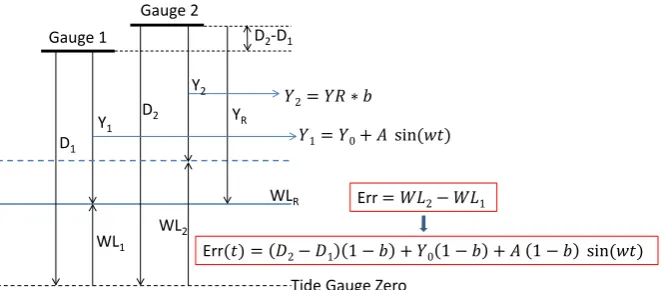
Fig. 2. Scheme used to explain how the presence of a scale error (b6=1) in a water level time series (WL2)introduces an additional term in the bias or mean difference between the time series and the real or reference time series (WL1). In the example, the datum difference (D2−D1) is assumed to be due to the sensor position, but it could be also due to different tide gauge zero or to a combination of both. Err(t) is the error or difference between the two time series, composed of a constant term and a variable term (sinusoidal variation as the typical tide, for example). This constant term is related to the bias and varies with the datum difference, the scale errorband the set-up of the station Y0(distance of the sensor to mean sea level).

As mentioned at the beginning of this section, there are two main types of sources of error: (a) those due to instru-mental/installation problems, and (b) those due to physical and environmental influences. The former may sometimes be corrected so we will describe next some of them and their influence on the sea level data during the renovation of the REDMAR network.

2.1 The scale error influence

One common source of error when measuring sea levels is related to tide gauges systematically measuring sea levels different to the real ones by a factorε(the so-called scale-error), with differences increasing with the distance to the sensor. When comparing with other sensors, this can be seen as a trend on the Van de Casteele plot (Lennon, 1968; IOC, 1985; Martín Míguez et al., 2008), and quantified from the slope of the linear fit between the two time series of sea lev-els asε=(b−1)×100, withbbeing the slope of the linear fit.

Although radar sensors may of course have their own scale error, it has been proved that this is much lower than the one from acoustic or pressure sensors. In the test station in Vila-garcía (Martín Míguez et al., 2005), the values of scale error were less than 0.1 % between the MIROS radar and two dif-ferent acoustic sensors, an Aquatrak loaned by NOAA (Na-tional Oceanic and Atmospheric Administration, US) and the SRD one from the REDMAR network.

A scale error in a sea level time series introduces a bias with respect to the original time series. This is easy to show, for example, if we consider a reference time series of sensor to water distance asy1=y0+Asin(t /T ), wheret is time, and a second time series,y2=b∗y1, affected by a scale er-ror determined byb. Ify0=300 andA=200, for example,

this roughly corresponds to a set-up similar to existing sta-tions in the north of Spain, where the sensor is located around 300 cm above the maximum tide level and the tidal amplitude is 200 cm (T is chosen to be equal toM2period: 12.47 h). If these two time series are converted to water level, WLi, by

differences between each datum to the measured distances, (in our example we can useD1=399 cm,D2=400 cm, and a scale error of 2 %, i.e.b=1.02) the bias between the two time series WL2 and WL1becomes −5.98 cm, which does not match the datum difference (D2−D1=1.0 cm). This is so because the bias between two time series will depend not only on datum differences but also on the scale error, the nominal distances of the sensors above mean sea level mea-sured at station set-up, and on the tidal range (this can be con-firmed for the mentioned example by the exact expression of the error WL2–WL1, which can be easily obtained following the scheme in Fig. 2). In summary, in order to match the mean level of two different time series of sea level measured at the same location, but where a scale error might be present, an estimation of such scale error and understanding its influence in the bias is needed.

2.2 Time shifts

Another source of error is the time shift due to clock mal-function. This was a common error present in old tide gauges but not in the modern ones, such as the new stations of RED-MAR, as they include a GPS receiver for time assignment, one of the main requirements of the new MIROS-based sta-tions. The detection of this problem is easy and is reflected in an increased standard deviation of the differences (Stdv).

(5)

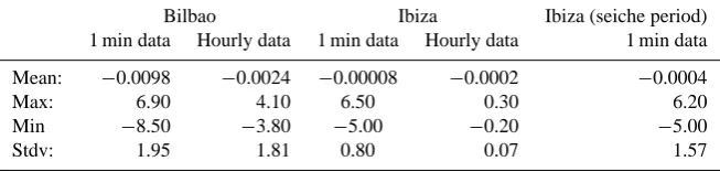
Table 1. Statistics of differences (in cm) between original and 2 min shifted time series for Bilbao and Ibiza (one month of data). Results

are presented both for 1 min time series and for filtered hourly values. An additional computation is made for a few days with important “seiches” in Ibiza (last column).

Bilbao Ibiza Ibiza (seiche period) 1 min data Hourly data 1 min data Hourly data 1 min data

Mean: −0.0098 −0.0024 −0.00008 −0.0002 −0.0004

Max: 6.90 4.10 6.50 0.30 6.20

Min −8.50 −3.80 −5.00 −0.20 −5.00

Stdv: 1.95 1.81 0.80 0.07 1.57

Balearic Islands) were artificially delayed by 2 min. The ex-periment was made for one month of 1 min data in both cases. Differences between the original time series and the delayed one were then analysed and basic statistics computed, both for the original 1 min data and for the filtered hourly values (Table 1).

The table shows that a standard deviation of up to 1.8 cm for hourly values can be explained by just a 2 min shift at Bilbao, where the maximum tidal range is around 5 m. How-ever, at Ibiza, where there is a tidal range less than 20 cm, the same time shift would produce an increase of only 0.07 cm in the standard deviation for hourly values. While the esti-mated errors relative to the tidal range are similar (1.8/500≈ 0.07/20≈0.0035), the observed increase of 0.07 cm at Ibiza is one order of magnitude less than the uncertainty on wa-ter level datum differences and therefore well within the ex-pected uncertainty rangeO(1 cm) (see section about uncer-tainty on water elevation relation to datum). Larger values of Stdv will be obtained from 1 min time series differences in Ibiza and other Mediterranean stations with small tidal range during periods with larger “seiches” and resonance effects (right column of Table 1). Filtering to hourly values during these events significantly reduces the standard deviation of the differences (from 1.57 to 0.10 cm in the example).

Time shifts will be reflected of course in differences in the phases of the main harmonic tidal constituents. The presence of a clock malfunction will be evident if the stations are at the same location and more difficult to determine if there is some delay in the tide due to a different position or because of a lag stemming from the particular instrumentation (e.g. a blocked well in a conventional gauge). However, this error does not generate a bias so it is not so important for long-term mean sea level studies.

2.3 Datum changes and drifts

Datum or reference connection between the tide gauges is one of the basic and critical steps for a successful renovation of a sea level station. Unfortunately, other errors may mask this connection, such as the scale error mentioned above. High precision levelling between the contact points of the two sensors is needed, something that would require more expense and time if they are not at the same location. The

bias or mean difference between the two water level time se-ries should be practically zero once other sources of error such as the scale error have been eliminated. A trend in these differences will indicate the presence of a drift in one of the gauge datums, something very important for study of lower frequency climate or geological processes (secular trends), if this drift would be unnoticed and uncorrected for a period much longer than a year.

2.4 Effective density effects in pressure sensors

Pressure sensors, placed in the water below the lower low water mark, measure the hydrostatic pressure above them, requiring the estimation of the density of the seawater prior to the calculation of the sea level from the pressure measure-ment. In the particular case of the REDMAR pressure sen-sors (AAND), the influence of barometric pressure is com-pensated for by applying air pressure to one side of the trans-ducer through an air pipe and compensating unit. The AAND sensors operate with a predefined constant value of density, determined during the installation phase for each station. This means that there is a potential influence of density vari-ations on the derived sea level data.

(6)

2.5 Air temperature effects in acoustic sensors

Acoustic sensors, located a few metres above the water sur-face, measure the travel time of acoustic pulses reflected ver-tically from the air/sea interface to derive the distance to the water surface and then the sea level height relative to a datum. This travel time depends on the determination of the speed of sound, which varies with the air conditions, especially with temperature gradients. In principle, the speed of sound is esti-mated in the SRD sensors before each measurement, using a calibration measurement over the first 1 m of range from the sensor. However, the sea level measurement itself requires knowing the speed of sound over the full range, and this value may not correspond well to the calibrated one. The sensors measure inside protective tubes painted white to avoid tem-perature gradients along the tube in larger tidal regimes. Er-rors in their operation will be reflected in an increased scale error and lower precision of the sensor during low waters compared to during high waters. On the other hand, the tem-perature gradients will vary throughout the year, leading to seasonal variations of the scale error that may become evi-dent when comparing the acoustic sensors with radar sensor data (as a seasonal signal in the mean sea levels differences).

2.6 Delamination problem in radar antennas

One of the main problems in the comparison of old and new tide gauges in the REDMAR network became apparent af-ter a detailed study of sea level data at Algeciras harbour (Gibraltar Strait), in May 2010. This new station, based on a MIROS radar sensor, was installed in the summer of 2009. Real-time quality control procedures at that time showed an apparently good performance of the antenna. However, when data from the Spanish Institute of Oceanography in Algeciras Bay and from the National Oceanography Centre Liverpool tide gauge at Gibraltar were compared with the MIROS sen-sor, an apparent slow rise of mean sea level during several hours became evident in the MIROS data with respect to the other two tide gauges. After that, the mean sea level relative to these sensors became stable and remained a few centime-tres above the original signal. Figure 3 shows the effect of delamination on the daily means at Algeciras and its correc-tion after replacing the antenna in July 2010.

An inspection of the MIROS installation at Algeciras re-vealed the existence of a problem in the MIROS antenna. After contacting the manufacturer we were informed that this was a potential problem of a set of antennas provided to REDMAR, basically consisting of a failure in the glue joint of the two circuit boards that form the antenna, allowing air to enter inside the joint and thus starting a delamination pro-cess.

As a consequence of this, an immediate plan of verification and substitution of all the installed MIROS radar sensors was put in place in collaboration with the maintenance company and the manufacturer. At the same time, new calibration and

31 Fig. 3. Influence of de-lamination in daily mean sea levels at Algeciras harbour. Daily means 1

from the REDMAR MIROS station (blue) are lower than the daily means from IEO tide 2

gauge (red), due to their datum difference. During the period the MIROS antenna was de-3

laminated (shown by the green arrow), mean sea levels from REDMAR became larger than 4

the IEO ones. The problem disappeared after MIROS antenna replacement in July 2010, when 5

the IEO sea levels became higher again (and the difference constant). The effect is clear in the 6

differences time series. 7 8 9 10 11 12 13 14 15 16 17 18 19

Fig. 3. Influence of delamination in daily mean sea levels at

Al-geciras harbour. Daily means from the REDMAR MIROS station (blue) are lower than the daily means from IEO tide gauge (red) due to their datum difference. During the period the MIROS antenna was delaminated (shown by the green arrow) mean sea levels from REDMAR became higher. The problem disappeared after MIROS antenna replacement in July 2010, when the IEO sea levels became higher again (and the difference constant). The effect is clear in the differences time series (black line).

real-time monitoring procedures were established for these sensors to avoid a potential repetition of the problem. Up to 11 of the 17 antennas of the MIROS devices that were installed to replace the older tide gauges have shown evi-dence of delamination with different degrees of impact on the data (Fig. 4, red periods show data affected by delamination). All the REDMAR MIROS stations have been replaced at the time of writing of this paper, independently of the detection of delamination problems, following the manufacturer’s ad-vice.

3 Data and methods

3.1 Stations and data description

Seventeen pairs of tide gauges stations are used (Fig. 1 and Table 2), four of them based on pressure sensors (AAND) and the rest on acoustic (SRD) sensors. The location of the new radar station might be at the same or at a different location inside the harbour, the latter sometimes unavoid-able due to harbour works and development (e.g. Valencia and Barcelona). Other times, the reason for relocation was more related to the interest of monitoring higher frequency phenomena such as agitation (Vigo, Málaga or Motril sta-tions). Available periods of overlap for comparison range from 120 days to more than three years, although just the segment where both stations were working properly is used (Fig. 4).

(7)

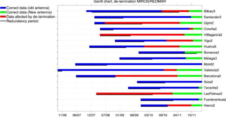
32 Fig. 4. Gantt chart showing the period of operation of the MIROS radar sensors installed to 1

replace an old REDMAR station (black line is the overlapping period). Red: period of data 2

affected by the de-lamination problem in the new sensors. All the stations have now the new 3

model of antenna (green, Motril and Ibiza replaced in 2012). Blue: data not affected by de-4

lamination. As can be seen red periods do not always coincide with the overlapping period. 5

6

7

8

9

10

11

12

13

14

15

16

17

18

Fig. 4. Gantt chart showing the period of operation of the MIROS radar sensors installed to replace an old REDMAR station (black line is the

overlapping period with the old sensor). Red: period of data affected by the delamination problem in the new sensors. Blue: data not affected by delamination. As can be seen red periods do not always coincide with the overlapping period. All the stations now have the new model of antenna (green: Motril and Ibiza replaced in 2012).

Raw data consist of 1 min averages for MIROS radar sen-sors and of 5 min data for the AAND and SRD sensen-sors. The 1 min radar data were averaged to 5 min sampling in order to make the comparisons with the older tide gauges. However, it is important to take into account that the SRD 5 min value corresponds to a mean of around 40 s of multi-ple echoes within the 5 min, and that the AAND 5 min value corresponds to the average of last 5 min of 1 s measurements. Use of subsampling instead of a 5 min average has been tried in the radar data (not possible for the older ones) for two of the stations, Huelva (SRD sensor and large tidal range) and Ibiza (AAND sensor and very small tidal range), but no important differences in the statistical results of the compar-isons have been found. The MIROS strategy will be the one adopted in the future, so it seems reasonable to look for dif-ferences in the overall final products without considering the subsampling.

After detailed quality control, the data used for this study are some of the products generated by Puertos del Estado on a regular basis for all the tide gauges of the Spanish RED-MAR network: the 5 min (minimum standard data sampling of the old tide gauges), hourly, daily and monthly averaged sea level time series. We will focus then on the coherence of processes with frequencies lower than 0.1 cycles min−1. De-tailed tide gauge benchmark information was used to analyse the differences observed between time series concerning da-tum connection.

3.2 Comparison method

The first step consists of the visualization of the time series of the differences (Fig. 5), and the computation of the fol-lowing basic statistical descriptors: bias or mean difference, standard deviation (Stdv), 50 % percentile (p50), maximum and minimum difference (Rmax, Rmin) and Pearson’s correla-tion coefficient,R. For the hourly and daily time series, and for the same time period, the linear trend is also computed, and the slope given with its 68 % confidence interval (±one standard deviation).

A linear fit, y=a+bx, between the two time series is calculated to estimate the scale error from the slope of the linear fit asε=(b−1)×100. The Van de Casteele plots for the 5 min, hourly, daily and monthly averages are then ob-tained. These should present a tilt or inclination for 5 min and hourly values if the scale error value is related to differences in the tidal range. If the scale error in the old time series is corrected, this inclination disappears. In other cases, the inclination is not present, indicating a different origin of the scale error or the inclination appears in the daily and monthly means instead due to seasonal variations.

(8)

Table 2. Stations upgraded within the REDMAR network, including relative positions of the old and new tide gauges (on the same or on

another quay of the harbour), type of old sensor, redundancy period for the comparison studies and main problems from the new and old sensors (delamination in the MIROS antennas or malfunction of the old sensor).

Location Type Old/New Overlapping (days) Delamination Malfunction

short names period MIROS old sensor

Bilbao Different SRD Bilb/Bil3 20090603–20100112 1189 Yes No Santander Same SRD Sant/San2 20080206–20090317 397 No No Gijón Same SRD Gijo/Gij2 20080208–20080701 323 Yes No Coruña Same SRD Coru/Cor2 20080425–20081028 184 No Yes Villagarcía Different SRD Vill/Vil2 20080424–20090624 423 Yes No Vigo Different SRD Vigo/Vig2 20081120–20091231 358 No No Huelva Same SRD Huel/Hue5 20080101–20081231 361 No No Bonanza Same SRD Bona/Bon2 20100113–20101113 487 No Yes Málaga Different SRD Mala/Mal3 20090122–20100423 411 No No Motril Different AAND Motr/Mot2 20070922–20080802 208 No Yes Valencia Different SRD Vale/Val3 20060801–20061114 120 No Yes Barcelona Different SRD Barc/Bar2 20071231–20081030 310 No No Ibiza Same AAND Ibiz/Ibi2 20090924–20101018 374 No Yes Tenerife Same SRD Tene/Ten2 20090522–20100812 427 No Yes Las Palmas Different SRD LasP/Las2 20090101–20100429 766 Yes No Fuerteventura Different AAND Fuer/Fue2 20091112–20110207 357 No No Hierro Different AAND Hier/Hie2 20091114–20100615 361 No Yes

the ones in the Atlantic coast). Notice that the entire time series is used for this computation even though the clocks of pressure and acoustic sensors were checked and synchro-nized every three months during in situ maintenance. This method was used as a first approximation of the time shift and was later compared with the observed values of this time shift during maintenance.

3.2.1 Uncertainty on water level relation to a datum

Knowing the uncertainty associated to the sea level measured by each type of sensor is key for analysing the overlapping time series. This uncertainty will depend not only on the type of instrument but also on the procedure followed to convert raw measurements to water level relative to a datum. Figure 6 shows a general scheme to convert distance measurement to water level relative to a datum, in the case of acoustic and radar sensors located above the water surface. According to this, datum definition will have its own uncertainties that will stem from, among other sources, the ability of the field tech-nician to adjust the datum (not lower than 1 cm), the level-ling error between the tide gauge bench mark (TGBM) and the sensor contact point (which is 0.03 cm for the REDMAR network), the repeatability of measurements (depending on the sensor) and the variability of environmental conditions. Taking all these sources of error into account and using the propagation error theory, we have calculated a total uncer-tainty of the datum definition of 0.15 cm for the MIROS radar sensor, 1.012 cm for the acoustic SRD sensor and 1.41 cm for the AANDERAA pressure sensor.

From the discussion above and, provided no other sources of error or malfunction are present, datum determination will be more precise for the MIROS stations than for the older tide gauges in REDMAR. This will also imply that bias differ-ences below 1.4 cm in the case of AAND sensors and below 1.0 cm in the SRD sensors will be within this uncertainty.

3.2.2 Tide and surge comparison

A change of instrumentation may also affect the tidal har-monic constants and the meteorological residuals in a tidal analysis computation, two basic products from a tide gauge station. One of the critical functions of the REDMAR net-work, as for other sea level networks in the world, is the com-putation of the astronomical tide at each harbour and thereby the prediction of future tidal levels. No less important is also the use of tide gauge data for validation of storm surge fore-casts. For the latter, a meteorological residual time series is computed by subtracting the tide from the observations. In Puertos del Estado this validation is performed in near-real time (each 12 h) within the NIVMAR Sea Level Forecast System (Alvarez Fanjul et al., 2001), and a simple scheme of post-processing is used to correct the meteorological sea level forecast provided by a numerical model, by comparison with the residual time series obtained from each tide gauge for the last few days.

(9)

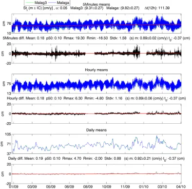
33 Fig. 5. Graphical representation of the inter-comparison, including basic statistics, for Málaga

1 (SRD) vs Málaga3 (MIROS) stations. The slope of the linear trend (

m

) is converted to

cm/y

.

2 The trend of both time series is similar (around 9

cm/y

), indicating no drift in either of the

3 stations. Average time shift estimated from the main tidal period,

∆

t

(

12 h

),

is 111.39 s.

4

5

6

7

8

9

10

Fig. 5. Graphical representation of the comparison, including basic statistics, for Málaga (SRD) vs. Málaga3 (MIROS) stations. The slope of

the linear trend (m) is converted to cm yr−1. The trend of both time series is similar (around 9 cm yr−1), indicating no drift in either of the stations. Average time shift estimated from the main tidal period is 111.39 s.

the redundancy period varies from 4 months to more than a year, the number of significant harmonic constants obtained will also be slightly different in each case. Results will be presented regarding the differences in the main tidal con-stituents and the residual or surge component for the two overlapping series at each station.

3.2.3 Impact of the renovation on historical mean sea levels – use of altimetry data

Another basic objective of a sea level network is the study of long-term mean sea level changes, for which daily, monthly and annual means are routinely computed from all tide gauges around the world. Monthly mean sea levels are com-piled by the Permanent Service for Mean Sea Level (PSMSL) due to its interest in global climate change impact studies

(Woodworth and Player, 2003). From the small amplitude of long-term mean sea level changes in a historical record (sev-eral millimetres per year), it is particularly important to have a good datum connection and a careful study of the influence of instrumentation and/or location changes in a network.

(10)

34 Fig. 6. Details of converting distance measurement from the acoustic SRD (left) and the 1

MIROS radar (right) to water level relative to the datum (WL). The SRD measures inside a 2

PVC tube to filter waves. Uncertainty in the datum (related to uncertainty in the levelling to 3

the contact point and datum definition) and the distance measurements from the different 4

sensors (YMIR and YSRD) will influence the final accuracy of water level measurements (WL).

5

6

7

8

9

10

11

12

13

14

15

16

17

18

Fig. 6. Details of converting distance measurement from the acoustic SRD (left) and the radar MIROS (right) to water level relative to the

datum (WL). The SRD measures inside a PVC tube to filter waves. Uncertainties in the datum (related to uncertainty in the levelling to the contact point and datum definition) and in the distance measurements from the different sensors (YMIRandYSRD)will influence the final accuracy of water level measurements (WL).

in the future, i.e. differences or biases of a few centimetres that may go unnoticed in operational applications.

Even stations that have been moved to another quay in the harbour should present practically the same behaviour in daily and monthly means as for the old one. Nevertheless, the situation is not always perfect and these are the many reasons for eventual differences in mean sea levels: imperfect datum connection, wrong operation or drift in one of the sensors, and differential vertical land movement of the station if lo-cated at a different quay. We can consider the scale error in one of the sensors as one of the second type of reasons be-cause, as explained in Sect. 2.1, this usually results in a bias in the means.

One way of checking the reliability of this historical time series is comparing data with nearby stations (buddy check-ing), as seasonal and interannual variations should be similar. Taking into account the problem of delamination that caused additional bias in the mean sea levels during the last years in some MIROS antennas, altimetry data in the vicinity of each tide gauge have also been used as an external source of information.

Altimetry sea surface height time series in the vicinity of each tide gauge have been computed from AVISO Sea Level Anomaly (SLA) maps (http://www.aviso.oceanobs. com). These are gridded data obtained combining up to four different satellite altimetry missions at a given time (up-dated time series, based on Topex/Poseidon/Jason-1/Jason-2/Envisat/GFO), which significantly increases the estimation of mesoscale signals (Le Traon and Dibarboure, 1999; Le Traon et al., 2001; Pascual et al., 2006), and that cover ex-actly the time period of the REDMAR network (since 1992 to present). We have used the global grid for the stations in

the Atlantic coast, with a spatial resolution of 1/3×1/3◦ and a higher resolution grid available for the Mediterranean stations (1/8×1/8◦). In both cases the temporal resolution is seven days. These are final products provided by AVISO so they have all the environmental and instrumental correc-tions applied, including the inverse barometer and higher fre-quency meteorological effects (Dynamic Atmospheric Cor-rection (DAC)). In order to compare with the tide gauge monthly means, we have eliminated this correction in altime-try data by adding again the DAC correction also provided by AVISO. As the DAC grid was not coincident with the SLA grids, an interpolation to the same grid was made. The al-timetry time series in the vicinity of each tide gauge has been obtained, averaging both data sets to monthly means, adding the two components, and computing the spatial mean on a small grid of 0.5◦resolution near the harbour. There is a gen-eral good agreement in the variability of altimetry and tide gauge time series obtained in this way (correlation values range from 0.8 at Motril to larger than 0.9 at the northern coast and Canary Islands stations).

(11)

land, long-term trends may also differ significantly due to lo-cal, regional or global land movements in the tide gauge. All these signals may represent themselves differently at differ-ent locations and are difficult to determine, but this concern is not included in the scope of this work. Altimetry time se-ries here are only intended to help in the identification of sig-nificant changes during the upgrade of technology or sensor and to check the continuity of the monthly means at the tide gauge station.

4 Results and discussion

4.1 5 min data, hourly values and daily means

Tables 3, 4, 5 and 6 summarize the main statistical results of the comparison study for the 5 min, hourly, daily and monthly means respectively. Before making an interpretation of these data, it is very important to emphasize that, first, all of them are average estimates for the whole overlapping pe-riod and, second, that they have been computed maintaining the original sampling and time assignment strategy of the dif-ferent sensors. This means that these values present an upper limit of the error and will be larger initially than what would be obtained from a more precise pre-processing of the time series.

Paying attention first to the bias column of Tables 3 to 6, it becomes evident which stations are already reasonably re-ferred to the same datum. This is the case for Huelva, Vigo, Santander, Málaga, Barcelona, Las Palmas and Hierro. The rest show bias ranging from 9.67 cm in Valencia to 1.23 cm in Tenerife (for the 5 min averages). For the stations where the sensors are at the same location (Ibiza, Coruña, Santander, Gijón and Bonanza) the bias should be related to scale er-ror, malfunction or wrong datum assignment. The rest of sta-tions may also show the influence of the different location in some way, although all of them have been connected by high-precision levelling and datum difference eliminated (Valen-cia and Motril, for example).

Woodworth and Smith (2003) stated that, provided the high-frequency noise in each of two compared sensors is of a similar magnitude, root mean square errors (in our case Stdv) values below 1.5 cm would yield a precision better than 1 cm for the individual sensors, which is consistent with Global Sea Level Observing System (GLOSS) stan-dards (IOC, 2002). Table 3 shows that for the 5 min data, only Barcelona would fulfil this condition and if we look for the stations with Stdv below 2 cm in the same table, this happens at Hierro, Fuerteventura, Las Palmas, Vilagarcía, Málaga and Valencia. This is interesting as all these tide gauges are in-stalled at different docks, so greater differences are expected to appear in the higher frequency phenomena. If we have a look to Table 4 (hourly values), then the GLOSS condi-tion would be fulfilled for five of the seventeen pairs of sta-tions: Las Palmas, Málaga, Motril, Barcelona and Valencia.

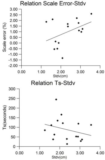
Fig. 7. Relation of scale error and time shift (Ts)with standard de-viation of the differences (Stdv) for each pair of stations. Stdv nor-mally increases for larger scale error (top) and decreases for smaller time shift (bottom). Anomalous values of scale error andTsin Va-lencia and Ibiza not included here.

Of these five, four are based on SRD sensors, one (Motril) is based on a pressure sensor, and only Las Palmas, in the Canary Islands, has a relatively high tidal regime; in all these cases, as previously stated, the MIROS station is located in a different location inside the harbour. As expected, averaging the 5 min data to hourly, daily and monthly means progres-sively reduces in general the Stdv parameter.

This seems to indicate that there is not a clear correlation of the Stdv with the distance between the two sensors or the type of sensor, being apparently more related to the good per-formance during the period of study. In fact, the particular value of Stdv depends on both the scale error and the time shift (Fig. 7), not corrected here, e.g. we have to look at these Stdv values as upper limits to the error. In Las Palmas, Gijón, Bilbao and Barcelona, a MIROS delamination problem was present during or immediately after the overlapping period, but a correct determination of the influence on the data and their correction has been possible.

(12)

Table 3. Results obtained from the 5 min averaged time series. (Stdv: standard deviation of the differences,Rmax: maximum difference, Rmin: minimum difference,R: correlation coefficient,ε: scale error (%),Ts: average time shift from M2period).a, b:yintercept and slope of the regression fit.

St1/St2 Bias Stdv Rmax Rmin a b R ε Ts

(cm) (cm) (cm) (cm) (%) (s)

Bil3/Bilb 4.72 3.04 29.90 −19.70 2.33 1.0099 1.00 0.99 28.76 San2/Sant −0.75 2.90 11.50 −24.90 −5.85 1.0178 1.00 1.78 51.85 Gij2/Gijo −2.57 2.36 36.80 −34.70 −6.60 1.0147 1.00 1.47 13.65 Cor2/Coru −2.14 2.35 12.60 −16.60 −6.73 1.0169 1.00 1.69 39.94 Vil2/Vill 1.52 1.71 8.20 −11.50 1.27 1.0011 1.00 0.11 −49.00 Vig2/Vigo −0.71 2.92 32.90 −22.80 −3.03 1.0111 1.00 1.11 −119.32 Hue5/Huel 0.23 3.10 26.30 −29.70 −2.30 1.0125 1.00 1.25 36.91 Bon2/Bona 5.01 3.30 20.60 −17.00 0.32 1.0261 1.00 2.61 112.50 Mal3/Mala 0.18 1.58 19.30 −16.50 −1.16 1.0210 1.00 2.10 111.39 Mot2/Motr −3.06 2.08 24.50 −46.40 −2.55 0.9867 0.99 −1.33 165.78 Val3/Vale 9.67 1.97 23.05 −4.35 14.58 0.9579 0.98 −4.21 267.13 Bar2/Barc −0.81 1.26 15.50 −10.30 −1.40 1.0188 0.99 1.88 84.90 Ibi2/Ibiz 1.25 2.15 13.00 −7.60 4.42 0.9210 0.98 −7.90 121.67 Ten2/Tene 1.23 2.57 42.40 −38.50 −2.29 1.0226 1.00 2.26 51.90 Las2/LasP −0.01 1.67 8.70 −22.00 0.86 0.9946 1.00 −0.54 37.45 Fue2/Fuer 4.26 1.89 24.50 −14.20 4.24 1.0001 1.00 0.01 135.01 Hie2/Hier −0.30 1.82 7.50 −12.40 0.50 0.9950 1.00 −0.50 244.81

Table 4. Results obtained from the hourly averaged time series. (Stdv: standard deviation of the differences,Rmax: maximum difference, Rmin: minimum difference,R: correlation coefficient,ε: scale error (%)).a, b:yintercept and slope of the regression fit.

St1/St2 Bias Stdv Rmax Rmin a b R ε

(cm) (cm) (cm) (cm) (%)

Bil3/Bilb 4.70 2.28 12.10 −5.30 2.30 1.0099 1.00 0.99 San2/Sant −0.76 2.76 5.80 −10.40 −5.86 1.0178 1.00 1.78 Gij2/Gijo −2.55 1.78 5.50 −10.90 −6.52 1.0145 1.00 1.45 Cor2/Coru −2.15 2.04 4.30 −12.00 −6.76 1.0170 1.00 1.70 Vil2/Vill 1.52 1.60 7.30 −5.00 1.26 1.0012 1.00 0.12 Vig2/Vigo −0.71 2.54 8.90 −11.10 −3.02 1.0111 1.00 1.11 Hue5/Huel 0.23 2.82 8.50 −9.80 −2.32 1.0126 1.00 1.26 Bon2/Bona 5.01 3.04 16.90 −10.40 0.30 1.0262 1.00 2.62 Mal3/Mala 0.18 1.16 6.30 −4.80 −1.50 1.0264 1.00 2.64 Mot2/Motr −3.06 1.04 1.90 −6.90 −2.90 0.9959 1.00 −0.41 Val3/Vale 9.72 1.12 14.35 2.45 13.71 0.9658 0.99 −3.42 Bar2/Barc −0.81 0.95 2.50 −4.00 −1.47 1.0212 1.00 2.12 Ibi2/Ibiz 1.24 2.01 6.70 −5.10 4.36 0.9221 0.98 −7.79 Ten2/Tene 1.19 2.14 17.10 −13.40 −2.37 1.0229 1.00 2.29 Las2/LasP −0.02 1.44 6.20 −9.50 0.81 0.9950 1.00 −0.52 Fue2/Fuer 4.25 1.70 15.80 −6.30 4.25 1.0000 1.00 0.00 Hie2/Hier −0.29 1.78 4.70 −5.90 0.49 0.9951 1.00 −0.49

±3.3 min except at Valencia and Hierro; the large value ofTs at Valencia is not realistic due to the small amplitude of the semidiurnal tide (T =12.42 h), the period used for its com-putation. As mentioned before, clock malfunctions related to these time shifts are expected to come from the old sensors, as there is practically no shift for the MIROS GPS control of time. This has of course been checked and confirmed in the routine visits to the stations.

4.2 The scale error origin and effects

(13)

Table 5. Results obtained from the daily averaged time series. (Stdv: standard deviation of the differences,Rmax: maximum difference,Rmin: minimum difference,R: correlation coefficient).a, b:yintercept and slope of the regression fit.

St1/St2 Bias Stdv Rmax Rmin a b R

(cm) (cm) (cm) (cm)

Bil3/Bilb 4.69 1.49 8.00 0.20 12.40 0.9681 0.99 San2/Sant −0.76 1.72 2.80 −5.80 −9.04 1.0289 0.99 Gij2/Gijo −2.58 0.52 −1.20 −4.50 −4.01 1.0052 1.00 Cor2/Coru −2.17 0.66 −0.80 −3.90 0.58 0.9898 0.99 Vil2/Vill 1.50 0.93 4.10 −0.90 3.31 0.9916 0.99 Vig2/Vigo −0.69 0.83 2.10 −3.60 −0.16 0.9975 1.00 Hue5/Huel 0.24 1.99 4.50 −4.50 −4.37 1.0228 0.96 Bon2/Bona 4.99 1.11 8.00 2.10 8.77 0.9790 1.00 Mal3/Mala 0.19 0.88 4.70 −2.00 −2.45 1.0414 1.00 Mot2/Motr −3.06 0.64 −0.30 −4.30 −3.41 1.0093 1.00 Val3/Vale 9.73 0.73 11.15 7.75 14.22 0.9615 1.00 Bar2/Barc −0.79 0.68 1.10 −2.30 −1.43 1.0202 1.00 Ibi2/Ibiz 1.25 1.85 5.10 −2.20 4.75 0.9121 0.98 Ten2/Tene 1.20 0.79 3.40 −1.60 −0.19 1.0090 0.99 Las2/LasP −0.03 0.52 1.40 −1.70 4.19 0.9738 1.00 Fue2/Fuer 4.27 0.71 6.90 2.00 9.17 0.9682 0.99 Hie2/Hier −0.29 0.41 1.40 −1.40 −0.21 0.9995 1.00

Table 6. Results obtained from the monthly averaged time series. (Stdv: standard deviation of the differences,Rmax: maximum difference, Rmin: minimum difference,R: correlation coefficient).a, b:yintercept and slope of the regression fit.

(cm) (cm) (cm) (cm)

Bil3/Bilb 4.87 0.90 5.70 3.20 15.02 0.9580 0.99 San2/Sant −0.47 1.48 1.60 −2.70 27.20 0.9035 0.90 Gij2/Gijo −2.77 0.15 −2.60 −2.90 −12.21 1.0345 1.00 Cor2/Coru −2.45 1.03 −1.80 −4.40 22.60 0.9075 0.96 Vil2/Vill 1.42 0.76 2.60 0.20 1.81 0.9982 0.98 Vig2/Vigo −0.60 0.70 1.30 −1.50 2.59 0.9847 1.00 Hue5/Huel 0.23 1.99 2.90 −3.70 −14.87 1.0746 0.92 Bon2/Bona 4.90 0.83 6.30 3.70 14.95 0.9443 1.00 Mal3/Mala 0.25 0.46 1.30 −0.40 −2.91 1.0492 1.00 Mot2/Motr −3.19 0.25 −2.80 −3.60 −3.99 1.0209 1.00 Val3/Vale 9.95 0.70 10.45 9.15 31.51 0.8153 1.00 Bar2/Barc −0.84 0.58 0.00 −1.60 −1.98 1.0360 1.00 Ibi2/Ibiz 2.08 1.30 4.00 0.10 8.45 0.8327 0.99 Ten2/Tene 1.13 0.81 2.70 0.30 −19.28 1.1312 0.98 Las2/LasP −0.02 0.39 0.50 −0.90 7.31 0.9552 1.00 Fue2/Fuer 4.14 0.60 4.70 2.90 25.25 0.8639 0.99 Hie2/Hier −0.13 0.40 0.40 −0.70 1.78 0.9881 0.99

inside the harbours, and will more probably be related to instrumental problems for those stations located at exactly the same position: Santander, Gijón, Coruña, Huelva, Bo-nanza, Ibiza and Tenerife. For example, the estimated scale error derived from the 5 min and hourly time series does not differ significantly for all the Atlantic stations but it is sys-tematically different for the Mediterranean stations, Motril, Málaga, Valencia and Barcelona, where higher frequency

variability may differ more due to the “seiches” effect and different resonance responce at different harbour docks.

(14)

Table 7. Bias (from hourly values) and scale errorε(from 5 min and hourly values) for all the stations. Fourth column contains the distance in metres between the old and the new station and the fifth column the evidence of the scale error in the Van de Casteele plot. The scale error is clear in 7 stations (bold), all of them based on SRD sensors. Additional unexplained bias remains in some stations (*).

Station Bias Scale errorε Distance Influence Van (cm) 5 min/hourly (%) SRD/AAND-MIROS(m) de Casteele

Bilb* 4.70 0.99/0.99 1000 Yes Sant –0.76 1.78/1.78 0 Yes Gijo –2.55 1.47/1.45 5 Yes Coru –2.15 1.69/1.70 0 Yes

Vill 1.52 0.11/0.12 313 No

Vigo −0.71 1.11/1.11 250 No

Huel 0.23 1.25/1.26 0 Yes Bona 5.01 2.59/2.62 0 Yes

Mala 0.18 2.10/2.64 180 No

Motr* −3.06 −1.33/−0.41 600 No

Vale* 9.72 −4.21/−3.42 2500 No

Barc −0.81 1.88/2.12 915 No

Ibiz 1.24 −7.90/−7.79 0 No

Tene 1.19 2.26/2.29 0 Yes

LasP −0.02 −0.54/−0.52 523 No

Fuer* 4.25 0.01/0.00 422 No

Hier −0.29 −0.50/-0.49 125 No

particularly large negative values. In the case of Valencia, as mentioned above, this is probably due to real differences in the higher frequency signals, very important here where the distance between tide gauges is 2.5 km and the new sensor is much more exposed to wind waves. The large scale error in Ibiza (−7.9 % for 5 min averages), however, should be in-terpreted as a consequence of the difference in the seasonal cycle, due to a feature of the pressure sensor that does not take into account the changes of density through the year. For these reasons, both Valencia and Ibiza values of scale error were not included in Fig. 7.

Table 7 summarizes the bias, the scale error and its influ-ence in the Van de Casteele plots for the overlapping period. The table shows that the effect is clear in 7 of the stations, all of them based on SRD sensors, confirming that these sen-sors measured slightly lower low waters. When they are cor-rected, the bias between the time series falls well within the uncertainty limits defined for datum definition in each type of tide gauge and coincides with the existing datum differ-ence after levelling at 10 of the stations. Unexplained biases remain in the rest.

Looking into the detail in Table 7 and the Van de Casteele plots (Fig. 8) before and after correction of the scale error (slope of the regression fit), one can classify the influence of the scale error in the data according to the following situa-tions:

– Case A: stations with scale error>0.9 %:

– Case A1: the Van de Cateele plots show a clear inclination for the 5 min and hourly levels (not for the daily means), revealing a difference in the

tidal range. Correction of the scale error elim-inates this inclination and generates a bias be-tween the original and corrected time series for Bilbao, Santander, Gijón, Coruña, Huelva, Bo-nanza and Tenerife (Fig. 8, upper plot: Gijón sta-tion).

– Case A2: the Van de Casteele plots do not show inclination of the time series and the scale error correction only generates a bias between original and corrected time series (5 min, hourly and daily means) for Vigo, Málaga, Valencia, Barcelona and Ibiza. Figure 8 (middle plot) shows an ex-ample of this situation for Vigo. Ibiza is a special case; an inclination in the daily means, coherent with a seasonal variation observed in the daily means differences, disappears when correcting its large scale error, revealing only a significant bias change in all the time series (Fig. 8, bottom plot).

– Case B: stations with scale error<0.9 %: Vilagar-cía, Las Palmas, Fuerteventura, Hierro and Motril (for hourly values).

(15)

Fig. 8. Van de Casteele plots for 5 min, hourly and daily values for the original data (left panels) and for the same data after scale error

correction applied (right panel) for Gijón (top panel, case A1), Vigo (middle panel, case A2) and Ibiza (bottom panel, A2, special case). The value of the scale error in Ibiza is large (−7.79 % for hourly values) and results in a clear inclination in daily means, coherent with the differences observed in the seasonal cycle. Correction of this large scale error implies a significant bias change in all the time series.

AAND sensor at the end of its operation), Valencia (distance of 2.5 km between stations as well as datum problems in the historical SRD station) and Fuerteventura.

Of the 5 stations of case B (scale error below 0.9 %), only two are SRD-based stations (Vilagarcía and Las Palmas) and three AAND-based stations. Bilbao and Vigo present rela-tively small values of the scale error in comparison to the rest of the SRD stations. Interestingly, none of these new stations

(16)

In summary, a clear scale error appears in several SRD sensors, normally at stations with important tidal range (Ta-bles 3 to 7). Its influence affects basically the 5 min and hourly values and is reflected as a bias in the daily and monthly means. It seems reasonable to recommend trying its correction for the whole historical time series (in some cases 20 yr of data) if one wants to be certain about its reliability for providing accurate tidal products and extreme sea level anal-ysis. A small seasonal signal related to seasonal variations of temperature is apparent in the monthly and daily means at the SRD stations but its effect is negligible in the final trends, so we focus here in the mentioned bias that should be taken into account if it is larger than 1 cm (Sect. 4.4). Practically all the stations in the Mediterranean, where the tides are smaller, show little influence of the scale error in the hourly values but do present in some cases large differences in the 5 min data that the scale error correction eliminates. In all the cases ex-cept Ibiza station, this may be related to important physical differences in the signal because of the different location of the sensors, and it is not necessarily related to instrumental errors.

4.3 Results of tide and surge comparison

The scale error affects the tide computation with generally larger amplitudes for the semidiurnal constituents obtained from the SRD sensors. Table 8 contains the amplitude and phase of the main semidiurnal, diurnal and long-period har-monic constants for each pair of stations, obtained for the overlapping period. As already mentioned, the set of harmon-ics obtained differs slightly depending on the length of this period. For this reasonSaandSsaharmonic constants (annual and semiannual) are not available for some of the stations.

The main result from Table 8 is that practically all the sta-tions originally based on SRD sensors (except Las Palmas, Vilagarcía and Mediterranean stations with non-semidiurnal regime) show slightly lower (∼1–2 %) amplitude in the semidiurnal components (mainlyM2andS2)derived from the new MIROS sensor. This is consistent with the scale er-ror present at all these stations and, as explained, is due to the SRD sensors. This is something that does not happen when comparing with the pressure sensors (Hierro, Ibiza, Motril and Fuerteventura). In Ibiza station, however, there is a significant difference in the annual and semiannual (Saand Ssa)constituents, consistent with the problem detected in the pressure sensor, as explained in previous sections. The differ-ences in these constituents, when available, are related to ob-served seasonal variations in the differences at some acoustic and pressure sensors (notice however, the similar values of these constituents in all the pressure sensors except Ibiza).

Table 9 shows the statistical parameters of the compari-son of the residual time series for the same period (obtained from the previously obtained harmonic constants) and Fig. 9 shows the graphical comparison for Bilbao and Valencia. In the residual comparisons, a few spikes of±10 cm were

42 Fig. 9. Comparison of the hourly residual time series (blue for the new station, red for the old 1

one, black for the differences), for around 4 months of redundancy period at Bilbao and 2

Valencia 3

4

5

6

7

8

9

10

11

12

13

14

15

16

Fig. 9. Comparison of the hourly residual time series (blue for

the new station, red for the old one, black for the differences), for around 4 months of redundancy period at Bilbao (top) and Valencia (bottom).

identified and eliminated, although the results did not change significantly if they were included. These spikes were usu-ally related to the old station. Table 9 and Fig. 9 show a good performance for both tide gauges for storm surge applica-tions at practically all the staapplica-tions. The Stdv of the differ-ences is under 1.5 cm for 12 of the 17 stations. Bonanza, Bil-bao and Gijón present Stdv values greater than 1.8 cm (1.82, 1.83 and 1.89 cm respectively). The correlation index is nor-mally 0.98 or 0.99 except at Tenerife where it is 0.95. As the main problems seem to be related to deficiencies in the old stations (e.g. Tenerife, Coruña, Bonanza or Ibiza), this con-firms the capability of the new MIROS sensors to measure storm surges with sufficient accuracy. Nevertheless, in some cases there is an effect of high waves in the surge component, which is revealed by a sudden increase in the hourly residual of around 5 cm in the MIROS sensor. This is the case in Va-lencia, where sudden small surges were not recorded by the SRD, in a more sheltered and interior dock, but were mea-sured by the MIROS, closer to the mouth of the harbour and exposed to waves of more than 1 m during this time (Fig. 10). This could slightly affect extreme analysis studies, but not mean sea level, as we see in the next section.

4.4 Mean sea levels

(17)

Table 8. Main harmonic constants obtained from the two sensors for the overlapping period at each station. (SaandSsanot available at the stations where this overlapping period was too short).

Station M2 S2 O1 K1 SA SSA

Amp Phase Amp Phase Amp Phase Amp Phase Amp Phase Amp Phase (cm) (◦) (cm) (◦) (cm) (◦) (cm) (◦) (cm) (◦) (cm) (◦)

Bilb 131.96 92.88 46.15 122.86 7.13 320.31 6.47 70.35 7.34 134.44 Bil3 130.64 92.65 45.55 122.71 7.10 321.45 6.46 70.75 7.96 136.99 Sant 134.07 93.57 46.78 126.38 7.06 321.81 6.41 70.34 2.62 272.30 2.23 119.07 San2 131.76 93.28 45.94 125.95 6.92 321.53 6.17 70.30 1.81 320.40 2.29 113.50 Gijo 130.61 91.25 45.69 123.45 6.89 322.25 6.74 70.29 2.76 280.62 2.43 144.47 Gij2 128.74 91.38 44.93 123.45 6.80 322.80 6.53 70.36 3.17 297.08 2.79 141.65 Coru 120.01 86.63 40.77 116.43 6.55 323.84 7.86 72.50 1.69 42.48 Cor2 118.04 86.47 40.06 116.35 6.49 323.69 7.29 70.20 2.31 46.66 Vill 113.86 78.54 39.95 108.23 6.40 319.58 7.33 62.98 1.74 41.50 1.02 264.53 Vil2 113.82 79.17 39.63 108.84 6.38 319.89 7.29 62.75 2.00 23.84 0.89 235.06 Vigo 111.44 76.44 38.58 106.05 6.56 318.63 7.34 59.70 4.37 318.15 3.22 161.51 Vig2 110.12 77.44 38.41 106.86 6.45 319.00 7.07 62.43 4.60 320.79 2.81 159.44 Huel 105.34 57.06 38.50 83.83 5.76 310.34 6.37 46.62 4.74 224.38 1.99 49.69 Hue5 104.23 56.95 37.36 83.33 5.82 309.93 6.27 45.31 3.32 254.94 2.31 64.55 Bona 92.58 64.56 31.58 91.39 6.25 323.31 6.40 65.04 7.83 320.46 Bon2 90.11 63.64 30.41 90.73 6.21 322.62 6.23 62.49 8.22 320.79 Mala 19.17 49.95 7.37 74.67 1.76 120.76 3.19 151.72 4.13 293.48 2.33 274.92 Mal3 18.77 49.13 7.23 74.43 1.73 119.96 3.23 152.38 3.69 284.81 2.47 278.68 Motr 15.33 48.90 6.10 73.58 1.93 121.78 3.11 154.24 4.28 102.69 Mot2 15.49 47.64 6.06 73.56 1.91 121.82 3.25 152.47 4.29 105.17 Vale 1.77 196.19 0.55 158.08 2.26 107.60 3.72 162.72

Val3 1.86 198.04 0.68 193.60 2.37 109.08 3.59 168.30

Barc 4.63 213.11 1.72 227.29 2.36 103.50 3.75 166.25 5.29 110.03 Bar2 4.50 212.20 1.68 227.75 2.30 102.54 3.70 168.60 5.61 107.47 Ibiz 1.70 216.61 0.58 240.71 2.22 107.47 3.70 166.56 5.26 282.59 1.94 255.91 Ibi2 1.77 215.69 0.69 231.21 2.19 104.41 3.83 168.17 7.64 289.38 2.21 253.83 Tene 72.14 29.24 27.99 52.61 4.86 292.08 6.45 40.88 3.59 245.31 3.32 359.50 Ten2 70.68 28.61 27.23 52.52 4.77 292.16 6.17 39.62 2.84 247.83 3.15 0.62 LasP 75.44 28.58 29.02 52.92 4.94 293.13 6.19 40.33 3.78 276.86 2.18 15.00 Las2 75.92 28.13 29.03 53.05 4.93 292.37 6.24 40.53 3.93 276.46 2.40 18.27 Fuer 80.84 33.54 30.81 57.41 5.16 294.85 6.21 40.77 3.43 250.05 1.09 335.86 Fue2 80.81 32.32 30.61 56.26 5.17 293.82 6.13 39.21 3.92 247.06 1.30 333.50 Hier 59.54 23.26 24.69 47.70 4.31 291.69 6.15 32.97 2.39 110.81 Hie2 59.86 21.31 24.71 45.47 4.24 290.71 6.05 32.56 2.51 109.27

and especially for monthly means is much smaller than for 5 min and hourly values, so an individual wrong value will have a greater effect on the final statistics shown in these tables. The worst values are found for Huelva, Ibiza, Bil-bao, Santander and Coruña stations, in all the cases related to a seasonal signal in the SRD (related to seasonal varia-tions of the air-temperature effects in acoustic sensors) and AAND sensors (Ibiza case). Interestingly, some stations that presented important problems in the higher frequency and tidal analysis comparisons do not reveal large errors in these statistics. This is the case for Bonanza, for example.

Altimetry data have allowed a better determination of the impact on mean sea levels of problems that appeared in both the old and the new stations. For example, the delamination problem detected in many MIROS stations, most of the time

(18)

Table 9. Results obtained from the hourly residual time series. Stdv: standard deviation of the differences,Rmax: maximum difference,Rmin: minimum difference,R: correlation coefficient).a, b:yintercept and slope of the regression fit.

(cm) (cm) (cm) (cm)

Bilb/Bil3 0.01 1.83 8.60 −7.70 −0.01 0.9900 0.98 Sant/San2 0.05 1.26 6.20 −4.70 −0.05 1.0268 0.99 Gijo/Gij2 0.00 1.89 9.00 −7.40 0.00 0.9739 0.98 Coru/Cor2 0.04 1.02 7.70 −4.60 −0.04 1.0151 0.99 Vill/Vil2 0.05 1.13 5.20 −5.40 −0.05 0.9943 0.99 Vigo/Vig2 0.12 1.56 9.30 −7.30 −0.12 0.9940 0.99 Huel/Hue5 0.03 1.43 6.10 −5.40 −0.03 1.0024 0.98 Bona/Bon2 0.03 1.82 9.80 −9.60 −0.03 0.9778 0.99 Mala/Mal3 0.03 1.19 3.40 −6.50 −0.03 1.0398 0.99 Vale/Val3 0.16 1.05 7.00 −2.50 −0.16 0.9556 0.99 Ibiz/Ibi2 −0.13 1.05 3.30 −5.00 0.13 1.0025 0.99 Barc/Bar2 0.24 1.07 3.70 −3.30 −0.24 1.0271 0.99 Tene/Ten2 0.01 1.35 9.90 9.80 −0.01 0.9835 0.95 LasP/Las2 0.06 1.04 8.00 −6.90 −0.06 0.9754 0.98 Fuer/Fue2 0.06 0.82 3.00 −7.80 −0.06 0.9929 0.98 Hier/Hie2 0.01 0.81 4.40 −3.10 −0.02 0.9908 0.99

red, and the final time series in blue when the delamination bias was corrected. The trends (in cm yr−1) correspond to the period 1992–2011 and are significantly affected by this cor-rection (from 0.62 to 0.40 cm yr−1_{), which in this case yields} to a value closer to the altimetry trend. In the same way we have detected and corrected delamination problems in other stations like Barcelona, Gijón, Las Palmas or Vilagarcía.

Other times, the altimeter data helped to confirm a prob-lem in the old sensor instead. This is the case of Ibiza. Fig-ure 12 shows the comparison of monthly means from altime-try and from the tide gauge time series at this Mediterranean station, where the installation of the MIROS (data since Oc-tober 2009) clearly results in a better agreement with the al-timeter data. This is due to a problem in the seasonal cycle of the pressure sensor, already detected in other steps of the comparison.

Once all the stations were quality controlled in this way, the linear trends from altimetry and tide gauge monthly means for the same period of time were computed and are presented in Table 10. Although comparison of these two trends must be done carefully due to the differences ex-plained in Sect. 3.2, monthly means from the tide gauges have been used in other works for this purpose (García et al., 2012 ). The glacial isostatic adjustment (GIA) is the only component of land movement at the tide gauges that we know from the Peltier model (Peltier, 2004). The impact of GIA in the relative sea level change at each tide gauge has been added to Table 10, where it can be seen that its value is generally one order of magnitude smaller than the errors in our trends, so its correction is not relevant in this study. On the other hand, Ibiza is the only station with a Continu-ous Global Positioning System sensor providing information

Fig. 10. Wind waves recorded by the MIROS sensor (black, Hm0) plotted with the hourly 1

surge component (blue for the MIROS, red for the SRD) at Valencia harbor. Top: whole 2

redundancy period, bottom: just September 2006. The new sensor is placed in an exposed 3

area, the SRD in a rather closed dock and measuring inside a tube. There seems to be an small 4

effect of higher waves in the MIROS surge component. 5

6

7

8

9

10

11

12

13

14

15

16

17

Fig. 10. Wind waves recorded by the MIROS sensor (black, Hm0)

plotted with the hourly surge component (blue for the MIROS, red for the SRD) at Valencia harbour. Top: whole redundancy period, bottom: just September 2006. The new sensor is placed in an ex-posed area, the SRD in a rather closed dock and measuring inside a tube. There seems to be a small effect of higher waves in the MIROS surge component.

(19)

Table 10. Trends in cm yr−1obtained for the combined historical monthly means at each station without correcting the overlapping bias (4th column) and with correcting this bias (5th column). Altimeter trend for the same period, GIA component and GPS information, if available, have also been included. Rows written in bold show the stations where the bias significantly affects the computed sea level trend in the tide gauge; the * indicates for which stations the correction of the bias is recommended. An upward arrow in the last column indicates that the trend in the tide gauge is clearly larger than the one in the altimeter.

Station Nyears Bias overl. TG trend TG Trend with Altimeter GIA GPS period (cm) (cm yr−1) Bias (cm yr−1) trend (cm yr−1) (cm yr−1)

Bilbao* 19.50 4.72 0.10±0.08 0.26±0.08 0.20±0.07 –0.015 ↑ Santander 19.50 −0.75 0.21±0.08 0.17±0.08 0.21±0.07 −0.011

Gijón* 16.58 –2.57 0.18±0.11 0.08±0.11 0.01±0.09 –0.004 ↑

Coruña* 19.50 –2.14 0.22±0.09 0.13±0.09 0.23±0.07 0.0 –0.24±0.01 Vilagarcía* 14.67 1.52 0.42±0.14 0.53±0.14 0.18±0.10 –0.008 ↑ Vigo 19.17 −0.71 0.26±0.10 0.24±0.10 0.25±0.06 −0.012 −0.05±0.26 ↑ Huelva 15.25 0.23 0.40±0.11 0.40±0.11 0.35±0.09 −0.019 −0.19±0.5 ↑

Bonanza 19.50 5.02 0.63±0.08 0.77±0.09 0.39±0.06 –0.019 ↑

Málaga 19.50 0.18 0.47±0.07 0.47±0.07 0.38±0.08 −0.022 ↑

Motril 7.00 –3.06 0.40±0.31 –0.20±0.31 0.94±0.27 –0.020 ↑

Valencia 19.17 9.67 0.75±0.10 1.35±0.10 0.38±0.08 –0.011 –0.081±0.014 ↑ Barcelona 19.33 −0.81 0.67±0.09 0.64±0.09 0.30±0.10 0.003 ↑ Ibiza 8.92 1.25 0.82±0.25 0.98±0.25 0.45±0.27 0.014 −0.113±0.020 ↑

Tenerife* 19.42 1.23 0.65±0.07 0.69±0.07 0.38±0.06 0.008 ↑ Las Palmas 19.50 −0.01 0.60±0.05 0.60±0.05 0.36±0.05 0.005 −0.156±0.034 ↑

Fuerteventura 8.92 4.26 1.16±0.19 1.58±0.19 0.45±0.16 –0.001 ↑

Hierro 7.58 −0.30 1.63±0.27 1.58±0.27 0.71±0.23 0.009 ↑

were obtained for other harbours also from SONEL, but these stations are not close nor collocated with the tide gauge so the values must be taken only as a reference: in Huelva the er-ror of the trend is very large; in Coruña the subsidence itself is large (−0.24 cm yr−1_{) and reflects a very local movement} of the CGPS location (at another pier) not apparent in the tide gauge. The objective of Table 10 is to show the impact of correcting the overlapping period bias to the tide gauge time series; this correction is not needed, from the statisti-cal point of view, if the bias is smaller than 1 cm. This is the case for Santander, Vigo, Huelva, Málaga, Barcelona and Las Palmas. All these stations, except Huelva, have more than 19 yr of data, the longest periods in the network, so the stan-dard error of these trends is usually smaller. The correction is not significant in either Ibiza and Hierro, but in this case the error of the trend is larger because there are only 7 to 10 yr of data (as in Motril). The bias correction is significant for the following stations: Bilbao, Gijón, Coruña, Vilagar-cía, Bonanza, Motril, Valencia, Tenerife and Fuerteventura (bold formatted in the table). In summary, it seems that a bias equal to or larger than 1.5 cm may affect the trend for this length of time series (around 20 yr). The 4.7 cm bias in Bil-bao may be related to an error in the datum definition of the SRD, which could account for half of this difference, com-bined with the influence of the large distance between the stations (1 km). Valencia bias is known to be originated by a problem in the SRD sensor that is probably related to an ac-cidental change of datum during maintenance performed in

2003 rather than to harbour development, as has been stated in García et al. (2012). This error could explain at least 6 of the 9.67 cm of bias observed during the overlapping period. The rest could also reflect the large distance between the two tide gauges in Valencia (2.5 km) and also the very different wave and other environment conditions. Other stations with bias related to the old sensor are Bonanza (fresh water trap-ping in the SRD tube), Motril and Fuerteventura (wrong def-inition and inaccuracies of the pressure sensor) and Coruña, Gijón and Tenerife (clearly related to the scale error in the SRD).

The decision to apply this bias correction is not easy and clear-cut. It is not possible to know if the bias is due to a temporal problem in the old sensor affecting only the overlapping period, in which case the bias, although signifi-cant, should not be corrected, or if it is a constant bias due to the technology change. We think Bonanza, Motril and Fuerteventura could correspond to the first case; in fact the trends become less similar to the trends in the altimeter and other stations in the region if we apply the correction. How-ever this bias may be needed in Bilbao, Gijón, Coruña and Tenerife.

5 Conclusions