Does The Expectations
Hypothesis Explain The Term Structure
Of Treasury Bond Yields In Tunisia?
Jamel Boukhatem, Umm al-Qura University, Saudi Arabia and University of Tunis, Tunisia
ABSTRACT
This paper tests the expectations hypothesis (EH) using monthly data for Treasury bond yields (TBYs) over the period 1994m5–2014m12 and ranging in maturity from one year to 10 years. We apply cointegrated-VAR jointly on more than one pair of yields. The results suggest rejection of the EH throughout the medium maturity spectrum. However, for longer maturities they suggest the validity of the EH for the TBYs. This indeed confirms the smooth functioning of Tunisian bond market which gives an indication that the yield curve should serve as an indicator to the monetary policymakers to manage inflation and to influence the aggregate demand in the economy.
Keywords: Term Structure; Expectations Hypothesis; Bond Yields; Cointegrated VAR
1. INTRODUCTION
ond rates are essential conduits for the transmission of monetary policy. But bond rates contain bond trader expectations of future policy rates. Thus, monetary policy depends on the perception policy of the bond market, and the connection of these perceptions to the announced or recently observed policy is not fully understood.
On the theoretical level, a good theory of the interest rates term structure must explain not only the different structures of yield curves, but also the stylized facts demonstrated by many empirical studies (Mishkin, 2007). The theoretical foundations of the yield curve interpretation depend on the hypothesis made by each theory (pure expectations theory, segmented markets theory, liquidity prime theory and preferred habitat theory). The expectation theory of the term structure illustrated the idea that interest rates reflect the agents’ expectations on the financial markets (money and bond markets). In this case, long rates are expressed as a weighted average of expected future short rates. The term structure allows us then to determine whether there are possibilities of profitable arbitrage to be exploited in these markets.
Furthermore, the relation between short- and long-term interest rates is important for the monetary policy transmission mechanism. The monetary authority controls short rates, and if the case of a stable relationship between short and long rates will the authority also be able to control long rates and thereby stimulating real economic activity.
Likewise, the spread between long and short rates may contain useful information about future interest rates, inflation, and real economic activity. The monetary authorities may be able to use the yield spread as an indicator of the inflationary pressures in the economy. In total, the yield curve appears to be the main indicator of the dynamics of expectations.
Empirically, and far from being exhaustive regarding the presentation of empirical validation of the various theories of the interest rates term structure, we underline rather contrasting results. Indeed, the results depend not only on the country, period, data frequency and the maturity of the securities, but also and mainly on the rate expectations hypotheses and in determining the risk premium.
One of the most tested implications of the expectations theory of the term structure is that of Shiller (1979) which establishes that a longer-term bond rate is just the average of expected one-period rates for the duration of the bond plus some constant term premium. Empirical works overflow without making unanimity about the empirical validity of such a theory (Shiller et al. 1983; Campbell and Shiller 1987 & 1991; Engsted and Tanggaard 1994; Hall et al. 1992; Mankiw 1986; Hardouvelis 1994; Jondeau and Ricart 1999; Lanne 2000; Tzavalis 2003; Sarno et al. 2005; Thornton, 2006, etc.
However, other authors used the implications of the yield curve to measure the informational content of current rates on future rates. Thus, on the one hand, Mishkin (1991) and Jorion and Mishkin (1991) and Jondeau (2001) were interested by the information in the yield curve and, on the other hand, Fama and Bliss (1987) and Fama (1990) considered the information contained in the difference between future and spot rates.
An alternative approach to measure the predictive ability of interest rates based on the restricted vector autoregressive (restricted VAR, noted RVAR) proposed by Campbell and Shiller (1987 and 1988). This representation allows the deduction of forecasting short rates from the RVAR itself and thus to determine a long rate consistent with the expectations theory and the joint dynamics of interest rates. This approach provides a framework for coherent analysis with the statistical properties of interest rates. Since the works of Campbell and Shiller (1987) and Hall et al. (1992), many studies have highlighted the fact that interest rates are generally integrated and cointegrated pairs. In this case, the RVAR allows making several tests of the expectations hypothesis. The causality of the yield curve slope vis-à-vis changes in short and long rates is one of the most direct implications of the theory.
The aim of this paper is to study the relationship between short and long rates in order to identify a term structure of bond rates that can help banks, insurers, corporates and even investors to choose which bonds are bought and which ones will be sold. The rest of the paper is organized as follows. The second section will discuss modeling VAR applied to Tunisian Treasury bill rates (TTBR) used. The third section will focus on interpreting the various results. The fourth and final section concludes the paper.
2. THE VAR REPRESENTATION AND THE TEST OF THE EXPECTATIONS THEORY
In order to study the links between the TBR, we use the Vector Autoregressive model (VAR). To study the dynamics of interest rates, this representation was initially developed by Sargent (1979) and adapted by Campbell and Shiller (1987, 1988) for stationary differenced variables and cointegrated.
As mentioned above, the expectations theory based on the joint hypothesis of no arbitrage opportunities and rationality of expectations, argues that the yield at time t of a zero-coupon bond with a maturity n is equal to the average of the anticipated yields of successive investments: t, t + m, ..., t + n – m in bonds of maturity m (m < n), plus a constant term premium 𝜓#,%.
𝑅'%=)* -𝐸'𝑅',-## + 𝜓#,% (1)
𝑅'% is the n-period (long-term) rate 𝑅'#, is the m-period (short-term) rate ; 𝜓#,% is the constant risk premium that may vary with the maturity of the rates. 𝐸' is the expectations operator.
In this case, the expectations hypothesis represents the true data generating process. Also, expectations are rational so that:
𝐸'𝑅',-## = 𝑅',-## + 𝜈',-#
The term premium may depend on the maturity of the assets but is always constant over time. The term 𝐸'𝑅',- =
Hence, the forecasting of future rates, from equation (1), is possible provided that the term premium 𝜓#,% is stable while, some authors such as Evans and Lewis (1994) and Hardouvelis (1994) argue that this condition is not sufficient. Risk premiums must be constant to make good predictions about future rates1.
The first step in the process of Campbell and Shiller (1987, 1988) is to show that, in the context of a present-value model (Equation 1), the non-stationary short rate is reflected in the existence of a cointegrating relationship between short and long rates.
Thus, if we define the slope of the yield curve by 𝑆'#,%= 𝑅
'%− 𝑅'# (this slope is considered, by some authors, as the "spread" between the long rate and the short one), by subtracting 𝑅'# on both sides of the equation (1), we obtain the expression describing the relationship between the "spread", the expected changes in short-term rates and the risk premium:
𝑆'#,%=#
%𝐸' 𝑅',-#
# − 𝑅
'#
- + 𝜓#,% (2)
Noting that R7,899 − R79 = ∆R97,89+ R97,89;)+ ⋯ + ∆R97,) ; the equation (2) can be written as follows:
𝑆'#,%= 𝐸'𝑆'∗#,%+ 𝜓#,% (3)
Where the slope of perfect predicted rates S7∗9,? is defined by:
𝑆'∗#,%=# % ∆𝑅',@ # -# @A) - (4)
Equation 3 is fundamental in the analysis of the expectations theory since it establishes a link, proposed by Campbell and Shiller (1987, 1988), with cointegration. The interest of the interpretation in terms of co-integration consists to give to the expectations theory a suitable framework of statistical analysis. If short-term rates are stationary in difference, equations 3 and 4 shows that the curve slope (curvature of the yield curve) is stationary, since it depends on future changes in short rates (Equation 4). As short and long rates are cointegrated, it is possible to represent their joint dynamics using a VECM for changes in interest rates or RVAR for the change in short rates and the yield curve. Campbell and Shiller (1987, 1988) preferred the latter representation since it allows a simpler implementation of testing the expectations hypothesis.
Under the assumption that the dynamics of the process 𝑋'= (𝑅'# 𝑅'%)′ follows a VAR model of order p, it can be written as follows:
𝑋'= 𝛷E+ 𝛷)𝑋';)+ 𝛷F𝑋';F+ ⋯ + 𝛷G𝑋';G+ 𝜀' (5)
When all variables are centered, the VAR model can be written as follows to:
𝛷 𝐿 𝑋'= 𝜀'
Where 𝛷 𝐿 = 𝐼F− K-A)𝛷-𝐿- is a polynomial matrix in the lag operator 𝐿 characterized by: 𝐿*𝑋'= 𝑋';* , 𝐼% is the identity matrix with dimension n; 𝜀' is the vector of disturbances supposed white noise. 𝜀'= (𝜀),' 𝜀F,')′.
Note 𝛷 a matrix (2×2𝑝) containing the parameters of the VAR: 𝛷 = (𝛷)… 𝛷G). If it exists a cointegration relationship, the long term matrix 𝛷 1 = 𝐼F− K-A)𝛷- is written as the product 𝛷 1 = −𝛼 ∗ 𝛽′, where 𝛼 and 𝛽 two vectors of dimensions (2×1). 𝛽 is the cointegrating vector.
1
When interest rates are non-stationary but the slope of the yield curve is stationary, the cointegrating vector is written 𝛽 = (−1 1)′ , so that the slope plays the role of a restoring force with 𝛽S𝑋
'= 𝑅'%− 𝑅'#= 𝑆'#,%. We note 𝐻EU: 𝛽 = (−1 1)S.
Engle and Granger (1987) have shown that the dynamics of a system of non-stationary and cointegrated variables can also be studied as a vector error correction model (VECM) or a cointegrated VAR model (CVAR) for interest rates variations. In addition, Campbell and Shiller (1987, 1988) in bivariate cases, and Mellander et al. (1992) in multivariate cases, showed the equivalence between the VAR models in levels, the VECM model and the CVAR model under the expectations hypothesis.
Equation (5) can be expressed as an error or vector equilibrium correction model (VECM), i.e. a CVAR, which is formulated in terms of differences as follows:
Γ 𝐿 Δ𝑋'= 𝜇 + Π𝑋';)+ 𝜀'
⇔ Δ𝑋'= 𝜇 + Γ)Δ𝑋';)+ ⋯ + ΓG;)Δ𝑋';G,)+ Π𝑋';)+ 𝜀' (6)
The CVAR representation provides a favorable transformation as it reduces the multicollinearity problem often present in financial data by combining levels and differences. In addition, it allows distinguishing between stationarity that is created by linear combinations of the variables and stationarity created by first differencing. Finally, it gives an intuitive explanation of the data, categorizing the effects in long (Π) and short (Γ)) run information.
Consequently, we apply the CVAR model to test the expectations theory. This analysis could be useful in our context as it allows us to take account of the non-stationarity of the series, looking for cointegration properties in the data, while taking care of the feedback between the variables.
We use the two-step method proposed by Engle and Granger (1987). The first step consists at testing explicitly the cointegration rank and the value of the cointegration relationship’s parameter (long term relationship). In the second step, we estimate the dynamics of interest rates through the CVAR using the maximum likelihood procedure outlined in Johansen (1988) and Johansen and Juselius (1990).
The contribution of a CVAR is to find a specification that will keep the asymptotic normality of the estimators while keeping the level variables, and their long-term behavior. They involve the long-term relationships between the variables I(1), and the specified dynamic adjustment of the variables in differences. The Granger theorem shows the equivalence between the existence of "r" cointegrating vectors and the existence of CVAR.
To estimate the equation (6), we refer to Johansen (1988). Thus, if there’s "r" cointegrating vectors (0 < 𝑟 ≤ 𝑘)
between the composants of 𝑋', the matrix Π of rank r and dimension k can be decomposed as : Π = 𝛼𝛽S. The dimensions of 𝛼 and 𝛽 are (𝑘, 𝑟).
Δ𝑋'= 𝜇 + 𝛼𝛽S𝑋';-+ Γ-Δ𝑋 ';-*;)
-A)
+ 𝜀'
or,
Γ 𝐿 Δ𝑋'= 𝛼𝛽S𝑋';)+ 𝜀'
where Γ L = I?− c;)8A) Γ8L8 is of order (p − 1). 𝛼 represents the speed of adjustment coefficient of the CVAR and
𝛽 the matrix of long-term coefficients.
3. EMPIRICAL RESULTS
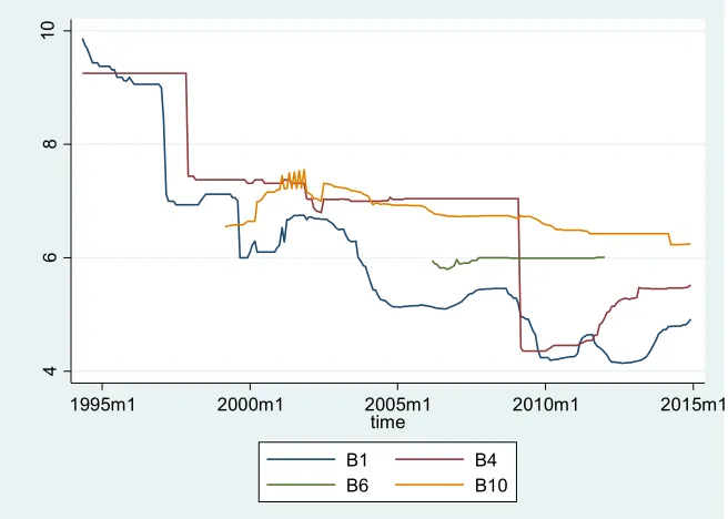
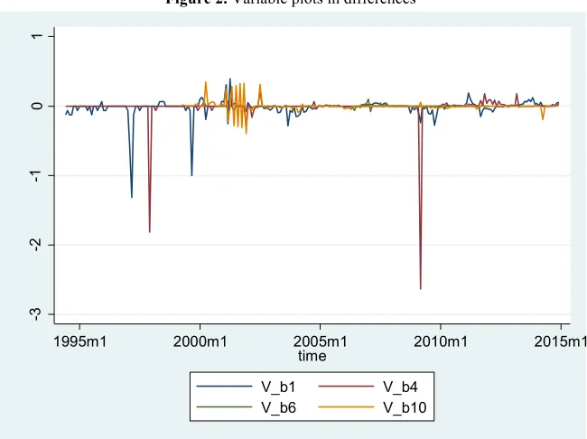
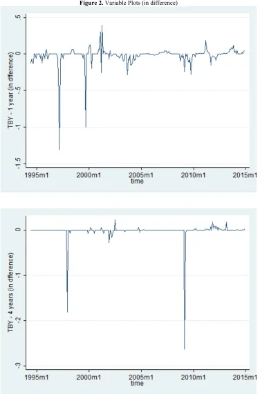
Empirically, the expectations hypothesis is tested from the cointegration between a short-term rate and long-term rate. In this study, cointegration is estimated between many pairs of Treasury bill yield (TBY) rates with one-year, three-year, four-year, six-year, seven-year and ten-year maturity. But, maturities which data are more available and more suitable in terms of autocorrelation will be chosen. Consequently, we retain, 1-year, 4-year, 6-year and 10-year maturity TBYs (appendix – fig. 1 & fig. 2)
𝑋'= (𝑏'), 𝑏
'f, 𝑏'g, 𝑏')E)′ is a (4×1) vector of endogenous I(1) variables where 𝑏'# is the yield at time 𝑡 of a zero-coupon bond with 𝑚 years to maturity. 𝑣_𝑏'# indicates the first difference of the corresponding variable.
The use of this range of interest rates takes into account the fact that expectations on future rates in the short-, medium- and long-term can be different, and, at the same time, to obtain information not only on the slope of the yield curve, but also and especially on the dominant form of the curvature. The sample covers monthly data from 1994:5 to 2014:12. The choice of this frequency is coherent with the related empirical literature.
Before testing for stationarity of the series, we present a graphical analysis for the series in levels and in differences. The figure 1 suggests that TBYs of the one-year, three-yea, six-year and ten-year maturity differ not so much in levels while the ten-year yield is typically higher than yields of short-term maturities. In differences, we show that the long-term yields are less variable. This could be explained according to the above presented theory that longer-term yields can at least partially be explained by the average expected current interest rates of all periods to maturity and thus contain information on the shorter end of the yield curve. This aggregation implies that long maturities are less affected by temporary shocks. TBYs also appear to be highly persistent, well approximated by I(1) process.
Figure 1. Variable plots in levels
4
6
8
10
T
BYs
in
le
ve
ls
1995m1 2000m1 2005m1 2010m1 2015m1
time
B1 B4
Figure 2. Variable plots in differences
To test for the stationarity, we use the augmented Dickey-Fuller test (ADF), the Phillips-Perron test (PP) and the modified Dickey–Fuller t test (known as the DF-GLS test) proposed by Elliott, Rothenberg, and Stock (1996).
For ADF and PP tests, the null hypothesis (Ho) consists at the existence of unit root against the alternative hypothesis of the absence of unit root in the series. The null hypothesis is accepted when the t-statistic exceed the critical value. However, if it is less, we reject the null hypothesis, the series are stationary. For the DF-GLS test, the null hypothesis is that the DGP is a random walk, possibly with drift.
Table 1 summarizes all results. For level-series stationarity, the results show that all series have a unit root and are thus non-stationary in levels but they are stationary in first differences and are considered as I(1).
Table 1. ADF, PP and DF-GLS tests for stationarity of TBYs
(i) (ii) (iii)
ADF PP ADF PP DF-GLS ADF PP DF-GLS
𝑏') -1.579 -1.959 -2.413 -2.554 0.427 -2.337** -2.551** -0.930
𝑏'm -1.925 -2.154 -1.451 -1.426 0.623 -3.202* -2.968* -1.836
𝑏'f -2.196 -2.321 -1.496 -1.510 -0.052 -1.438 -1.426 -2.234
𝑏'g -2.445 -1.584 -1.474 -2.679 -1.800 0.288 0.280 -2.280
𝑏'n -1.097 -0.171 -0.245 0.151 --- -0.250 -0.366 ---
𝑏')E -3.909** -3.638** -1.458 -0.926 -0.798 -0.340 -0.422 -0.801
𝑏')F 0.105 0.609 1.645 2.403 2.341 -1.651*** -1.696*** -0.181
𝑣_𝑏') -12.069* -12.113* -11.890* -11.957* -6.397* -11.705 * -11.796* -8.660*
𝑣_𝑏'm -11.549* -11.551* -11.521* -11.530* -7.484* -11.030* -11.110* -7.645*
𝑣_𝑏'f -15.419* -15.420* -15.432* -15.433* -10.57* -15.382* -15.385* -10.60*
𝑣_𝑏'g -9.465* -9.453* -9.552* -9.534* -0.742 -9.572* -9.534* -1.920
𝑣_𝑏'n -22.854* -29.241* -22.914* -29.310* --- -22.965* -29.305* ---
𝑣_𝑏')E -26.764* -24.438* -26.382* -23.851* -9.420* -26.426* -23.871 * -10.50*
𝑣_𝑏')F -12.553* -12.637* -12.182* -12.189* -7.994* -11.975* -11.975* -8.649*
* Significant at 1%; ** Significant at 5%; *** Significant at 10% (p-value less than 1%, 5% and 10%) (i) with intercept and trend ; (ii) with intercept ; (iii) without intercept
Critical levels in ADF and PP tests: (i) -4.01 (1%), -3.43 (5%) and -3.13 (10%). (ii) -3.46, -2.88 and -2.57. (iii) -2.58, -1.95 and -1.62. Critical levels in DF-GLS test: (ii) -2.580(1%), -1.950(5%) and -1.620(10%). (iii) -3.480, -2.890 and -2.570.
--- Series contain gaps.
-3 -2 -1 0 1 T BYs in d iff ere nce s
1995m1 2000m1 2005m1 2010m1 2015m1
time
V_b1 V_b4
According to these results and considering the existence of breakpoints in some series (3-year and 7-year maturity TBYs), we use 1-year, 4-year, 6-year and 10-year maturity TBYs that seem more adequate to test the EH of the term structure.
Since all series are I(1), it is possible to analyze, in the logic of Campbell and Shiller (1987, 1988), their cointegration properties, and this by estimating the following relationship:
𝛽)𝑏'#+ 𝛽F𝑏'%+ 𝛽m= 𝜀' (7)
The cointegration vector 𝛽 = (𝛽), 𝛽F, 𝛽m) is thus written as 𝛽E= (1, −1, 𝛽m), where the risk premium 𝛽m – constant over time – depends on the maturities 𝑚 and 𝑛.
Three models will be tested:
𝑀𝑜𝑑𝑒𝑙 1: 𝛽)𝑏')+ 𝛽F𝑏'f+ 𝛽m= 𝜀'
𝑀𝑜𝑑𝑒𝑙 2: 𝛽)𝑏')+ 𝛽F𝑏'g+ 𝛽m= 𝜀'
𝑀𝑜𝑑𝑒𝑙 3: 𝛽)𝑏')+ 𝛽
F𝑏')E+ 𝛽m= 𝜀'
The tests of the optimal lag based on Akaike, Schwarz, Hannan-Quinn and LR criteria systematically lead to keep 2 lags, of a maximum of 4, for the first two pairs of TBYs (𝑏), 𝑏f) and (𝑏), 𝑏g) and 3 lags for the pair (𝑏), 𝑏)E). These delays are those that minimize selected criteria (Table 2).
Table 2. Lags choice using Akaike, Schwarz and Hannan-Quinn
Criteria information
Lags 1 2 3
𝒃𝟏 – 𝒃𝟒 AIC -1.600 -1.641*
SBIC -1.514* -1.497
HQIC -1.565 -1.583*
LR 1812.9 17.985*
𝒃𝟏 – 𝒃𝟔 AIC -7.771 -7.944*
SBIC -7.574 -7.615*
HQIC -7.693 -7.814*
LR 413.82 19.565*
𝒃𝟏 – 𝒃𝟏𝟎 AIC -3.984 -4.364 -4.399*
SBIC -3.880 -4.190* -4.155
HQIC -3.942 -4.293 -4.300*
LR 1076.9 78.284 14.522*
AIC: Akaike information criterion ; SBIC: Schwarz Bayesian information criterion ; HQIC : Hannan–Quinn information criterion ; LR : likelihood-ratio.
Before presenting the results of cointegration tests between the different pairs of TBYs, we note that theoretically, two non-stationary variables X7 and Y7 I(1) are cointegrated if it exists between them a stationary linear combination I(2) . Thus, the linear combination: Z7= X7− βY7 is stationary; β is the cointegrating parameter and
(1, −β) is the cointegrating vector (Granger, 1981). In other words, the residuals of the regression between these two variables I 1 would, over time, a tendency to revert to a constant average. In many empirical cases, long-term relationship tends towards zero with time; at least this’s what probably happening in the context of our study.
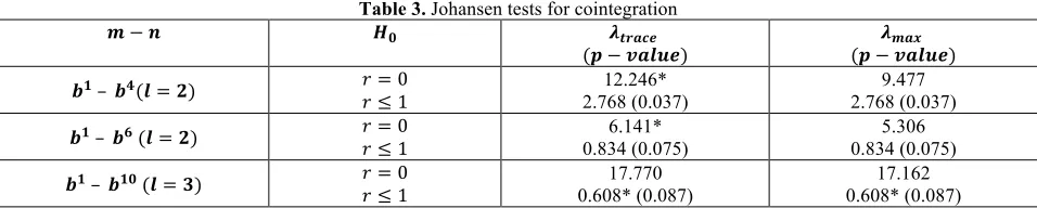
Table 3. Johansen tests for cointegration
𝒎 − 𝒏 𝑯𝟎 𝝀𝒕𝒓𝒂𝒄𝒆
(𝒑 − 𝒗𝒂𝒍𝒖𝒆) (𝒑 − 𝒗𝒂𝒍𝒖𝒆)𝝀𝒎𝒂𝒙 𝒃𝟏 – 𝒃𝟒(𝒍 = 𝟐) 𝑟 = 0
𝑟 ≤ 1 2.768 (0.037) 12.246* 2.768 (0.037) 9.477 𝒃𝟏 – 𝒃𝟔 (𝒍 = 𝟐) 𝑟 = 0
𝑟 ≤ 1 0.834 (0.075) 6.141*
5.306 0.834 (0.075) 𝒃𝟏 – 𝒃𝟏𝟎 (𝒍 = 𝟑) 𝑟 = 0
𝑟 ≤ 1 0.608* (0.087) 17.770 0.608* (0.087) 17.162
* signify the existence of cointegrating relationship. All models with constant trend.
According to the results in table 4 we accept the null hypothesis of no cointegration equations in the bivariate models 𝑏) – 𝑏f and 𝑏) – 𝑏g but there’s one cointegrating relationship between 𝑏) and 𝑏)E. Consequently, we accept the null hypothesis of the absence of cointegration relationship between the two pairs of variables. The absence of an eventual cointegration relationship is an argument for the reject of the EH of the term structure of TBYs for the mentioned maturities. This result is validated from both the trace statistics and maximum eigenvalue, and with deterministic trend or without in the cointegrating equation.
Econometrically, the absence of cointegration is a puzzling, but can be explained by the differences in basic logic growth of time series. Also, the frequency of observations and possible non-linearity of the relation could often explain the absence of cointegration (Engle and Granger 1991). The CVAR would be the better technique in estimating the dynamic processes of the variables for the models 1 and 2. However, we estimate the parameters of the VEC form for the model 3.
Results of the estimated parameters for model 3 are reported in table 4 below.
Table 4. Estimated parameters of the different models
Model 𝛂 𝛃 𝛍 𝚪
(b4 – b1)
(p-value) (-0.032, 0.020) (0.044, 0.036) (1, -1.101) (0.000) (-0.010, -0.016)
(0.441, 0.036) −0.032 0.2740.024 0.038∗ (b6 – b1)
(p-value) (0.057, -0.202) (0.25, 0.124) (1,0.045) (.419) (0.003, -0.001) (0.225, 0.903) −0.0670.202 0.4570.012∗ (b10 – b1)
(p-value (-0.056, 0.079) (0.003, 0.007) (1, -0.465) (0.000) (-0.005, -0.003)
(0.279, 0.619) 0.193
∗ 0.106 −0.056 0.153∗∗
* and ** : significant at 1% and 5%. LM test: Lagrange-multiplier test for autocorrelation, H0: no autocorrelation at lag order.
The results show the rejection of the EH for models 1 and 2: 1-year 4-year and 1-year 6-year maturity. This rejection implies that agents do not optimally use all available information to forecast short-term rates. Also, such a rejection can be explained by the presence of liquidity constraints and, maybe by the time variability of the term premium or market segmentation (Thornton 2005-2006, Dai and Singleton 2002, Tzavalis and Wickens 1997). The theory of market segmentation rejects the EH because it concluded that the expectations in short-term rates play no role in determining long-term rates. Similarly, the rejection of the EH can also be explained, theoretically, by the tightening of monetary policy. Indeed, when the monetary authorities decide to tighten monetary conditions, including in response to inflationary pressures, there is a rise in short-term rates, the long-term rates also increased but to a lesser measurement.
We must not lose sight that the rejection of the EH in the context of the theory of the term structure of TBYs, is a forewarning sign of recession. Three propositions are possible: i) the investors anticipation of similar difficulties for the Tunisian economy justifies the decrease of director rates; ii) the decrease of term premiums combined with low expected inflation, reflecting the credibility of the Central Bank; iii) an imbalance between supply and demand of long-term bonds. We believe that these three explaining elements are playing now.
When the predictions from the cointegrating equation are positive, 1-year TBY is above its equilibrium value because his coefficient in the cointegrating equation is positive.
The quasi-fixed exchange-rate regime adopted by Tunisian monetary authority may reinforce the predictability of short-term rates and thus explain why the EH is not rejected for long maturities.
To check whether we have correctly specified the number of cointegrating equations we test the stability of VECM. Generally, the companion matrix of a VECM with 𝐾 endogenous variables and 𝑟 cointegrating equations has 𝐾 − 𝑟
unit eigenvalues. If the process is stable, the moduli of the remaining 𝑟 eigenvalues are strictly less than one. The different graphs (appendix – fig. 3) show that all the eigenvalues lie inside the unit circle. The VECM satisfies stability condition.
4. CONCLUSION
From an original database covering the period 1994m5 to 2014m12, this work establishes a diagnosis on the validity of the EH for TBYs in Tunisia. The results show the rejection of the EH for short and medium maturity (1-year 4-year and 1-4-year 6-4-year) but for longer maturity (1-4-year 10-4-year) the EH is confirmed. Two explanations for this rejection are possible. The first is based on the existence of a variable risk premium over time. The second however is based on the over-reaction of long rates in relation to future short rates.
The validation of the EH is a strong argument towards the smooth functioning of Tunisian treasury bond market which gives an indication that the yield curve should serve as leading indicator to the monetary policy and the real economy.
AUTHOR BIOGRAPHY
Associate Professor, Jamel Boukhatem teaches Principles of Islamic Economics, Microeconomic analysis, Macroeconomic analysis and Statistics in the Faculty of Islamic Economics and Finance, Umm al-Qura University – Saudi Arabia since 2013. Prior appointments included the High Business School and the High School of Business and Economic Sciences, University of Tunis. Boukhatem holds a PhD on Financial Economics (University of Paris West Nanterre la Defense) and a Doctoral Thesis Supervisor (HDR) on Economics (University of Tunis El-Manar). His research focuses on applied economics and monetary and financial macroeconomics.
REFERENCES
Campbell J.Y. and Shiller R.J. (1988), « Interpreting Cointegrated Models », Journal of Economic Dynamics and Control, 12(2/3), 505-522.
Campbell J.Y. and Shiller R.J. (1987), « Cointegration and Tests of Present Value Models », Journal of Political Economy, 95(5), 1062-1088.
Culbertson J.M. (1957), « The Term Structure of Interest Rates », Quarterly Journal of Economics, 71(4), 485–517.
Culbertson J.M. (1965), « The Interest Rate Structure: Toward Completion of the Classical System», in The Theory of Interest
Rates, F.H. Hahn and P.R. Brechling eds., London.
Dai Q. and Singleton K.J. (2002), « Expectation Puzzles, Time-Varying Risk Premia, and Affine Models of the Term Structure »,
Journal of Financial Economics,63(3), 415-441.
Driffill J., Psaradakis Z. and Sola M. (1997), « A Reconciliation of Some Paradoxical Empirical Results on the Expectations Model of the Term Structure », Oxford Bulletin of Economics and Statistics, 59(1), 29-42.
Evans M.D.D. and Lewis K.K. (1994), « Do Stationary Risk Premia Explain It All? Evidence from the term structure » NBER
Working Paper, 3451.
Fama E.F. (1990), « Term-Structure Forecasts of Interest Rates, Inflation, and Real Returns », Journal of Monetary Economics, 25(1), 59-76.
Fama E.F. and Bliss R.R. (1987), « The Information in Long-Maturity Forward Rates », American Economic Review, 77(4), ) 680-692.
Fisher I. (1930), The Theory of Interest, New York: Macmillan.
Gerlach S. (1996), « Monetary Policy and the Behavior of Interest Rates: Are Long Rates Excessively Volatile? », BIS Working
Paper,34.
Economics and Statistics, 74(1), 116-126.
Hardouvelis G.A. (1994), « The Term Structure Spread and Future Changes in Long and Short Rates in the G7 Countries »,
Journal of Monetary Economics, 33, 2, pp. 255-283.
Hicks J.R. (1939), Value and Capital, 2nd ed., Oxford: Clarendon.
Johansen S. (1988), « Statistical Analysis of Cointegration Vectors », Journal of Economic Dynamics and Control, 12 (2-3), 231-254.
Johansen S. and Juselius K. (1990), « Maximum likelihood estimation and inference on cointegration with application to the demand for money », Oxford Bulletin of Economics and Statistics, 52(2), 169-210
Jondeau E. (2001), « La Théorie des Anticipations de la Structure par Terme permet-elle de Rendre Compte de l’évolution des Taux sur Euro-devise ? », Annales d’Economie et de Statistique, 62, 725–750.
Jondeau E. and Ricart R. (1999), « The expectations hypothesis of the term structure: tests on US, German, French, and UK Euro-rates », Journal of International Money and Finance, N°18, 139–174.
Jorion P. and Mishkin F.C. (1991), « A Multicountry Comparison of Term-Structure Forecasts at Long Horizons », Journal of
Financial Economics, 29(1), 59-80.
Kritzman M. (1993), « What Practitioners Need to Know about the Term Structure of Interest Rates », Financial Analysts
Journal, 49(4), 14-18
Kugler P. (1990), « The Term Structure of Euro Interest Rates and Rational Expectations », Journal of International Money and
Finance, 9(2), 234-244.
Lubochinsky C. (1990), Les Taux d’intérêt, 2ème édition, Dalloz.
Lutz F.A. (1940), « The Structure of Interest Rates », Quarterly Journal of Economics, 55(1), 36–63.
MacDonald R. and Speight, A.E. (1991), « The Term Structure of Interest Rates under Rational Expectations: Some International Evidence », Applied Financial Economics, 1(4), 211-221.
Mankiw N.G. (1986), « The Term Structure of Interest Rates Revisited », Brookings Papers on Economic Activity, 1986(1), 61– 96.
Meiselman D. (1962), The Term Structure of Interest Rates, Printice Hall Inc, Englewood Cliffs, New Jersey.
Mellander E., Vredin A. and Warne A. (1992), « Stochastic Trends and Economic Fluctuations in a Small Open Economy »,
Journal of Applied Econometrics, John Wiley & Sons, Ltd., 7(4), 369-394.
Mishkin F.S. (2007), The Economics of Money, Banking and Financial Markets, 8th ed., Pearson Education Inc. Addison-Wesley.
Mishkin F.C. (1991), « A Multi-Country Study of the Information in the Shorter Maturity Term Structure about Future Inflation
», Journal of International Money and Finance, 10(1), 2-22.
Modigliani F. and Sutch R. (1967), « Debt Management and the Term Structure of Interest Rates », Journal of Political
Economy, 75(4), 569-589.
Sargent T.J. (1979), « A Note on Maximum Likelihood Estimation of the Rational Expectations Model of the Term Structure »,
Journal of Monetary Economics, 5(1), 133-143.
Shiller R.J. (1979), « The Volatility of Long-Term Interest Rates and Expectations Theories of the Term Structure », Journal of
Political Economy, 87(6), 1190-1219.
Shiller R.J., Campbell J.Y. and Schoenholtz K.L. (1983), « Forward Rates and Future Policy: Interpreting the Term Structure of Interest Rates », Brookings Papers on Economic Activity, 1983(1), 173-223.
Thornton D. L. (2005), « Predictions of Short-term Rates and the Expectations Hypothesis of the Term Structure of Interest Rates », Federal Reserve Bank of St. Louis Working Paper, 2004-010A.
Thornton, D.L. (2006) « Tests of the Expectations Hypothesis: Resolving the Campbell-Shiller Paradox », Journal of Money,
Credit, and Banking, 38(2), 511-542.
APPENDIX
(Figure 2. Continued)
Figure 3. VAR/VECM stability
-1
-.
5
0
.5
1
Ima
gi
na
ry
-1 -.5 0 .5 1
Real
Roots of the companion matrix
Stability test of VAR(b4 - b1)
-1
-.
5
0
.5
1
Ima
gi
na
ry
-1 -.5 0 .5 1
Real
(Figure 3 continued)
-1
-.
5
0
.5
1
Ima
gi
na
ry
-1 -.5 0 .5 1
Real
The VECM specification imposes 1 unit modulus
Roots of the companion matrix