Inference for Approximating Regression Models

University of Pennsylvania

ScholarlyCommons

Publicly Accessible Penn Dissertations

1-1-2014

Inference for Approximating Regression Models

Emil Pitkin

University of Pennsylvania, [email protected]

Follow this and additional works at:http://repository.upenn.edu/edissertations Part of theStatistics and Probability Commons

This paper is posted at ScholarlyCommons.http://repository.upenn.edu/edissertations/1405

For more information, please [email protected].

Recommended Citation

Pitkin, Emil, "Inference for Approximating Regression Models" (2014).Publicly Accessible Penn Dissertations. 1405.

Inference for Approximating Regression Models

Abstract

The assumptions underlying the Ordinary Least Squares (OLS) model are regularly and sometimes severely violated. In consequence, inferential procedures presumed valid for OLS are invalidated in practice. We describe a framework that is robust to model violations, and describe the modifications to the classical inferential procedures necessary to preserve inferential validity. As the covariates are assumed to be

stochastically generated ("Random-X"), the sought after criterion for coverage becomes marginal rather than conditional. We focus on slopes, mean responses, and individual future observations. For slopes and mean responses, the targets of inference are redefined by means of least squares regression at the population level. The partial slopes that that regression defines, rather than the slopes of an assumed linear model, become the population quantities of interest, and they can be estimated unbiasedly. Under this framework, we estimate the Average Treatment Effect (ATE) in Randomized Controlled Studies (RCTs), and derive an estimator more efficient than one commonly used. We express the ATE as a slope coefficient in a population regression and immediately prove unbiasedness that way. For the mean response, the conditional value of the best least squares approximation to the response surface in the population - rather than the conditional value of y, is aimed to be captured. A calibration through pairs bootstrap can markedly improve such coverage. Moving to observations, we show that when attempting to cover future individual responses, a simple in-sample calibration technique that widens the empirical interval to contain $(1-\alpha)*100\%$ of the sample residuals is asymptotically valid, even in the face of gross model violations. OLS is startlingly robust to model departures when a future y needs to be covered, but nonlinearity, combined with a skewedX-distribution, can severely undermine coverage of the mean response. Our ATE estimator dominates the common estimator, and the stronger the R squared of the regression of a patient's response on covariates, treatment indicator, and interactions, the better our estimator's relative performance. By considering a regression model as a semi-parametric approximation to a stochastic mechanism, and not as its description, we rest assured that a coverage guarantee is a coverage guarantee.

Degree Type Dissertation

Degree Name

Doctor of Philosophy (PhD)

Graduate Group Statistics

First Advisor Lawrence D. Brown

Keywords

INFERENCE FOR APPROXIMATING REGRESSION

MODELS

Emil Pitkin

A DISSERTATION

in

Statistics

For the Graduate Group in

Managerial Science and Applied Economics

Presented to the Faculties of the University of Pennsylvania

in

Partial Fulfillment of the Requirements for the

Degree of Doctor of Philosophy

2014

Supervisor of Dissertation

Lawrence D. Brown

Miers Busch Professor of Statistics

Graduate Group Chairperson

Eric Bradlow

K.P. Chao Professor, Marketing, Statistics and Education

Dissertation Committee

Lawrence D. Brown, Miers Busch Profes-sor of Statistics

Richard A. Berk, Professor of Statistics and Criminology

Andreas Buja, Liem Sioe Liong/First Pacific Company Professor of Statistics

INFERENCE FOR APPROXIMATING REGRESSION MODELS

COPYRIGHT© 2014

Acknowledgments

I thank first Mama and Papa – Drs. Pitkin – together with Dedushka Rafa, Babushka

Rita, and Babushka Sonya. You were my first teachers. I learn from you always.

Love and reverence for your suffuses my every step. I dedicate this dissertation

to you. I thank my incomparable, good, and wise advisor Larry Brown, who is a

towering flame and who cultivated all my sparks, however slight. I thank Richard

Berk, Andreas Buja, Ed George, and Linda Zhao who have also generously and

significantly shaped my thinking as a statistician and this work. I thank my early

mentor Ken Stanley, whose unfailing trust and reservoir of wisdom has propelled me

on. I thank my classmates Alex Goldstein, Adam Kapelner, Justin Rising, Jordan

Rodu, Jose Zubizaretta, and also Justin Bleich. We few, we happy few! I thank the

members of the Salon and of the Captain’s Club. Words and equations and flint are

all the same – rub them the right way and the sparks will fly.

I thank Mr. Waldman and Moreh Shem for their love of learning and of teaching,

Ethan Schaff for being the best math teacher I ever had, Mr. Randall and Mr. Jarvis

for their perfect advice, Mr. Astrue for his frequent support, Dr. Fichtner for his

ABSTRACT

INFERENCE FOR APPROXIMATING

REGRESSION MODELS

Emil Pitkin

Lawrence D. Brown

The assumptions underlying the Ordinary Least Squares (OLS) model are regularly

and sometimes severely violated. In consequence, inferential procedures presumed

valid for OLS are invalidated in practice. We describe a framework that is robust

to model violations, and describe the modifications to the classical inferential

pro-cedures necessary to preserve inferential validity. As the covariates are assumed to

be stochastically generated (Random-X), the sought after criterion for coverage

be-comes marginal rather than conditional. We focus on slopes, mean responses, and

individual future observations. For slopes and mean responses, the targets of

infer-ence are redefined by means of least squares regression at the population level. The

partial slopes that that regression defines, rather than the slopes of an assumed

lin-ear model, become the population quantities of interest, and they can be estimated

unbiasedly. Under this framework, we estimate the Average Treatment Effect (ATE)

in Randomized Controlled Studies (RCTs), and derive an estimator more efficient

regression and immediately prove unbiasedness that way. For the mean response, the

conditional value of the best least squares approximation to the response surface in

the population rather than the conditional value of y, is aimed to be captured. A

calibration through pairs bootstrap can markedly improve such coverage. Moving to

observations, we show that when attempting to cover future individual responses, a

simple in-sample calibration technique that widens the empirical interval to contain

(1−α)∗100% of the sample residuals is asymptotically valid, even in the face of gross

model violations. OLS is startlingly robust to model departures when a futureyneeds

to be covered, but nonlinearity, combined with a skewedX-distribution, can severely

undermine coverage of the mean response. Our ATE estimator dominates the

com-mon estimator, and the stronger the R2 _{of the regression of a patient’s response on}

covariates, treatment indicator, and interactions, the better our estimator’s relative

performance. By considering a regression model as a semi-parametric approximation

to a stochastic mechanism, and not as its description, we rest assured that a coverage

Contents

1 Introduction 1

2 Random Predictors and Model Violations∗ 4

2.1 Abstract . . . 4

2.2 Introduction . . . 5

2.3 Discrepancies between Standard Errors Illustrated . . . 6

2.4 Populations and Targets of Estimation . . . 8

2.5 Observational Datasets and Estimation . . . 13

2.6 Decomposition of the LS Estimate According to Two Sources of Variation 15 2.7 Assumption-Lean Central Limit Theorems . . . 16

2.8 The Sandwich Estimator and the M-of-N Pairs Bootstrap . . . 18

2.9 Adjusted Predictors . . . 20

2.10 Proper and Improper Asymptotic Variances Expressed with Adjusted Predictors . . . 23

2.11 Discussion . . . 27

2.12 Proofs . . . 29

3.1 Abstract . . . 32

3.2 Introduction . . . 33

3.3 Neyman Framework, Fixed X, True Models . . . 35

3.4 Target of Estimation . . . 38

3.5 Illustration on real data . . . 54

3.6 Conclusion . . . 56

3.7 Technical appendix . . . 58

4 Calibrated Prediction Intervals 64 4.1 Abstract . . . 64

4.2 Introduction . . . 64

4.3 Marginally correct intervals . . . 67

4.4 Procedures . . . 72

4.5 Performance comparison . . . 74

4.6 Calibrated Intervals for the Mean Response . . . 76

4.7 Conclusion . . . 79

Bibliography 83

List of Tables

4.1 n = 100 . . . 76

4.2 n = 500 . . . 76

4.3 n = 1000 . . . 76

List of Figures

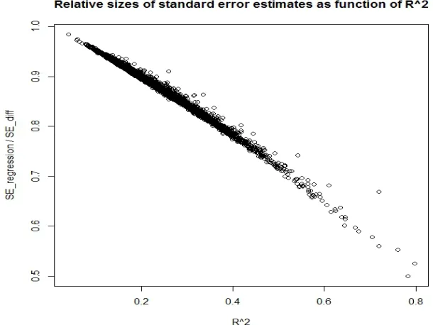
3.1 R2 plotted against SEˆ (_ˆτˆregression)

1

Introduction

The organizing principle of this work, which will be repeated in each chapter, is

two-fold: 1) that classical regression theory does not accommodate non-linearity or

heteroskedasticity in the presence of random predictors, and 2) that a re-examination

of the target of inference can and does give rise to valid, marginal inference.

Hal-bert White wrote a series of three papers (White, 1980b), (White, 1980a), (White,

1982) in which he addressed and solved the question of inference for misspecified

models. The sandwich estimator he introduced is asymptotically equivalent to the

non-parametric “pairs bootstrap,” which we will employ often in this work. Chapter

2, an adaptation of (Buja et al., 2013), examines this form of valid inference, which

includes a comparison of the relative performance of classical, or “conventional”

stan-dard errors, and those implied by the sandwich or the bootstrap. The key insight is

that regression slope estimates derived through OLS are asymptotically unbiased for

regression coefficients derived through population least squares. It is the randomness

of the joint distribution of the predictors and response that motivates the population

least squares procedure.

Chapter 3 changes orientation but preserves the statistical framework. We turn to

Randomized Controlled Trials (RCTs) and the attendant estimation of the Average

progenitor in Neyman’s thesis (Splawa-Neyman et al., 1990) to contemporary ones

that consider, as we do, semi-parametric settings (Zhang et al., 2008), (Rosenblum and

van der Laan, 2010), and then we explicitly define an estimator that is asymptotically

efficient relative to the difference in means estimator. Our estimator can be expressed

as a slope coefficient in a regression model of the sort defined in chapter 2, and

it is therefore asymptotically unbiased. This work sets a principled foundation to

the study of efficient ATE estimators, and admits many natural extensions to more

complex study designs.

The problem of predicting future observations in a regression setting without

in-voking normal-theory parametric intervals is not new. (Stine, 1985), for example,

examines the coverage of bootstrap prediction intervals. In his scheme the operating

assumption is that the model is correctly specified, and hence that the distribution of

the errors is known. (Schmoyer, 1992), who conscientiously avoids resampling

meth-ods, creates an estimator derived from a convolution of the empirical distribution of

the regression residuals. More resonant with our work, which assumes only a joint

distribution P between the X~ and y, and more recently, (Politis, 2013) states as a

common sense principle that in the absence of a model (the “model - free” case),

prediction intervals should be based on quantiles of the observed predictive

distri-bution. We adapt this principle to generate prediction intervals based on quantiles

of the empirical distribution of the residuals. In chapter 4 we show how a simple

in-sample calibration technique, which places minimal assumptions on the data

gen-erating process, gives desired, asymptotically valid coverage. Chapter 4 continues

with an exploration of valid coverage for the mean response. Again, our target of

inference is based on the population least squares approximation to the conditional

mean. We in simulations show examples where Xβ~ is covered with probability lower

theory are applied to misspecified models with random predictors. Again relying on

2

Random Predictors and Model Violations

Excerpted and adapted from Buja, A., Berk, Richard A., Brown, Lawrence D.,

George, Edward I., Pitkin, E., Traskin, M. Zhao, L., Zhang, K.: A Conspiracy of

Random X and Model Violation Against Classical Inference in Linear Regression.

2.1

Abstract

This chapter reviews the insights of Halbert White’s asymptotically correct inference

in the presence of “model misspecification.” This form of inference, which is pervasive

in econometrics, relies on the “sandwich estimator” of standard error. White permits

models to be “misspecified” and predictors to be random. Careful reading of his

theory shows that it is a synergistic effect — a “conspiracy” — of nonlinearity and

randomness of the predictors that has the deepest consequences for statistical

infer-ence. A valid alternative to the sandwich estimator is given by the “pairs bootstrap.”

We continue with an asymptotic comparison of the sandwich estimator and the

stan-dard error estimator from classical linear models theory. The comparison shows that

when standard errors from linear models theory deviate from their sandwich analogs,

they are usually too liberal, but occasionally they can be too conservative as well. The

chapter concludes by answering why we might be interested in inference for models

that are not correct.

2.2

Introduction

The classical Gaussian linear model reads as follows:

y = Xβ+, ∼ N(0N, σ2IN×N) (y,∈IRN, X ∈IRN×(p+1), β ∈IRp+1). (2.1)

Important for the present focus are two aspects of how the model is commonly

in-terpreted: (1) the model is assumed correct, that is, the conditional response means

are a linear function of the predictors and the errors are independent,

homoskedas-tic and Gaussian; (2) the predictors are treated as known constants even when they

arise as random observations just like the response. Starting with Halbert White’s

(White, 1980a), ((White, 1980b), (White, 1982)) seminal articles, econometricians

have used multiple linear regression without making the many assumptions of

clas-sical linear models theory. While statisticians use assumption-laden exact finite

sample inference, econometricians useassumption-lean asymptotic inference

based on the so-called “sandwich estimator” of standard error. The approach in this

chapter is to interpret linear regression in a semi-parametric fashion: the generally

nonlinear response surface is decomposed into a linear and a “residualized”

nonlin-ear component. The modeling assumptions can then be reduced to i.i.d. sampling

from largely arbitrary joint (X~, Y) distributions that satisfy a few moment

condi-tions. It is in this assumption-lean framework that the sandwich estimator produces

asymptotically correct standard errors.

boot-strap.” As the name indicates, the pairs bootstrap consists of resampling pairs (~xi, yi),

which contrasts with the “residual bootstrap” which resamples residuals ri.

Asymp-totic theory exists to justify both types of bootstrap under different assumptions

(Freedman, 1981), (Mammen, 1993). It is intuitively clear that the pairs bootstrap

can be asymptotically justified in the assumption-lean framework mentioned above.

In what follows we will use the general term “assumption-lean estimators of

standard error” to refer to either the sandwich estimators or the pairs bootstrap estimators of standard error.

The chapter concludes by comparing the standard error estimates from

assumption-lean theory and from classical linear models theory. The ratio of asymptotic variances

— “RAV” for short — describes the discrepancies between the two types of standard

error estimates in the asymptotic limit. If RAV 6= 1, then there exist deviations

from the linear model in the form of nonlinearities and/or heteroskedasticities. If

RAV = 1, then either the model is correct, or there has been a false negative.

2.3

Discrepancies between Standard Errors

Illus-trated

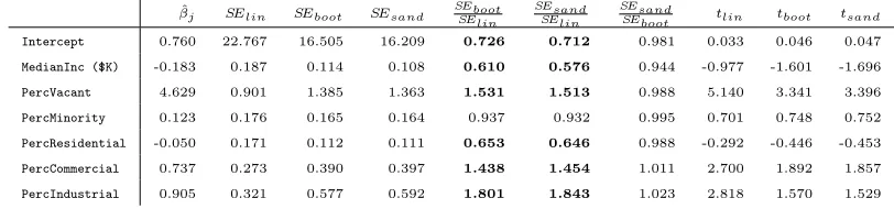
The table below shows regression results for a dataset in a sample of 505 census tracts

in Los Angeles that has been used to examine homelessness in relation to covariates

for demographics and building usage (Berk et al., 2008). We show the raw results

of linear regression to illustrate the degree to which discrepancies can arise among

three types of standard errors: SElin from linear models theory, SEboot from the pairs

bootstrap (Nboot = 100,000) and SEsand from the sandwich estimator (according to

(MacKinnon and White, 1985)). Ratios of standard errors are shown in bold font

Table 1: Regression coefficients along with their standard errors estimated by

different means.

ˆ

βj SElin SEboot SEsand SEboot_SElin SEsand_SElin SEsand_SEboot tlin tboot tsand

Intercept 0.760 22.767 16.505 16.209 0.726 0.712 0.981 0.033 0.046 0.047

MedianInc ($K) -0.183 0.187 0.114 0.108 0.610 0.576 0.944 -0.977 -1.601 -1.696

PercVacant 4.629 0.901 1.385 1.363 1.531 1.513 0.988 5.140 3.341 3.396

PercMinority 0.123 0.176 0.165 0.164 0.937 0.932 0.995 0.701 0.748 0.752

PercResidential -0.050 0.171 0.112 0.111 0.653 0.646 0.988 -0.292 -0.446 -0.453

PercCommercial 0.737 0.273 0.390 0.397 1.438 1.454 1.011 2.700 1.892 1.857

PercIndustrial 0.905 0.321 0.577 0.592 1.801 1.843 1.023 2.818 1.570 1.529

The ratios SEsand/SEboot show that the standard errors from the pairs bootstrap

and the sandwich estimator are in rather good agreement. Not so for the standard

errors based on linear models theory: we haveSEboot, SEsand > SElinfor the predictors

PercVacant, PercCommercial and PercIndustrial, and SEboot, SEsand < SElin for

Intercept,MedianInc ($1000),PercResidential. Only forPercMinorityisSElin

off by less than 10% from SEboot and SEsand. The discrepancies affect outcomes

of some of the t-tests: under linear models theory the predictors PercCommercial

and PercIndustrial have commanding t-values of 2.700 and 2.818, respectively, which are reduced to unconvincing values below 1.9 and 1.6, respectively, if the pairs

bootstrap or the sandwich estimator are used. On the other hand, for MedianInc

($K) the t-value −0.977 from linear models theory becomes borderline significant with the bootstrap or sandwich estimator if the plausible one-sided alternative with

negative sign is used.

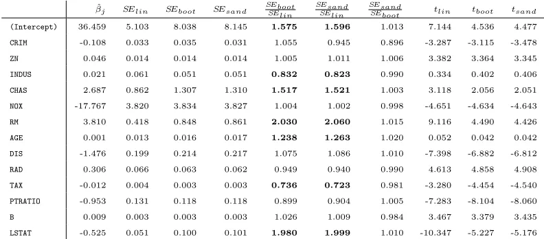
The second illustration of discrepancies between types of standard errors, shown in

the table below, is with the Boston Housing data (Harrison Jr and Rubinfeld, 1978).

We focus only on the comparison of standard errors. Here, too,SEboot andSEsand are

mostly in agreement as they fall within less than 2% of each other, an exception being

CRIM with a deviation of about 10%. By contrast, SEboot and SEsand are larger than

their linear models cousin SElin by a factor of about 2 for RM and LSTAT, and about

SEsandare only a fraction of about 0.73 ofSElinforTAX. Also worth stating is that for several predictors there is no substantial discrepancy among all three standard errors,

namely ZN, NOX, B, and even for CRIM, SElin falls between the somewhat discrepant values of SEboot and SEsand.

Table 2: Regression coefficients along with their standard errors estimated by

different means.

ˆ

βj SElin SEboot SEsand SEboot_SElin SEsand_SElin SEsand_SEboot tlin tboot tsand

(Intercept) 36.459 5.103 8.038 8.145 1.575 1.596 1.013 7.144 4.536 4.477

CRIM -0.108 0.033 0.035 0.031 1.055 0.945 0.896 -3.287 -3.115 -3.478

ZN 0.046 0.014 0.014 0.014 1.005 1.011 1.006 3.382 3.364 3.345

INDUS 0.021 0.061 0.051 0.051 0.832 0.823 0.990 0.334 0.402 0.406

CHAS 2.687 0.862 1.307 1.310 1.517 1.521 1.003 3.118 2.056 2.051

NOX -17.767 3.820 3.834 3.827 1.004 1.002 0.998 -4.651 -4.634 -4.643

RM 3.810 0.418 0.848 0.861 2.030 2.060 1.015 9.116 4.490 4.426

AGE 0.001 0.013 0.016 0.017 1.238 1.263 1.020 0.052 0.042 0.042

DIS -1.476 0.199 0.214 0.217 1.075 1.086 1.010 -7.398 -6.882 -6.812

RAD 0.306 0.066 0.063 0.062 0.949 0.940 0.990 4.613 4.858 4.908

TAX -0.012 0.004 0.003 0.003 0.736 0.723 0.981 -3.280 -4.454 -4.540

PTRATIO -0.953 0.131 0.118 0.118 0.899 0.904 1.005 -7.283 -8.104 -8.060

B 0.009 0.003 0.003 0.003 1.026 1.009 0.984 3.467 3.379 3.435

LSTAT -0.525 0.051 0.100 0.101 1.980 1.999 1.010 -10.347 -5.227 -5.176

Important messages are the following: (1) SEboot and SEsand are in substantial

agreement; (2)SElinon the one hand and{SEboot, SEsand}on the other hand can show

substantial discrepancies; (3) these discrepancies are specific to predictors. In what

follows we describe how the discrepancies arise from nonlinearities in the conditional

mean and/or heteroskedasticities in the conditional variance of the response given the

predictors. Furthermore, it will turn out that SEboot and SEsand are asymptotically

correct whileSElin is not.

2.4

Populations and Targets of Estimation

Before we compare standard errors it is necessary to define targets of estimation in

a semi-parametric framework. Targets of estimation will no longer be parameters

nonparametric class of data distributions. A seminal work that inaugurated this

approach is P.J. Huber’s 1967 article whose title is worth citing in full: “The behavior

of maximum likelihood estimation under nonstandard conditions.” The “nonstandard

conditions” are essentially arbitrary distributions for which certain moments exist.

A population view of regression with random predictors has as its ingredients

random variables X1, ..., Xp and Y, where Y is singled out as the response. At this

point the only assumption is that these variables have a joint distribution

P = P(dy,dx1, ...,dxp)

whose second moments exist and whose predictors have a full rank covariance matrix.

We write

~

X = (1, X1, ..., Xp)T.

for the column random vector consisting of the predictor variables with a constant 1

prepended to accommodate an intercept term. Values of the random vector X~ will

be denoted by lower case ~x= (1, x1, ..., xp)T. We write any function f(X1, ..., Xp) of

the predictors equivalently as f(X~) because the prepended constant 1 is irrelevant.

Correspondingly we also use the notations

P =P(dy,d~x), P(d~x), P(dy|~x) or P =P_Y,X~, P_X~, P_Y|_X~ (2.2)

for the joint distribution of (Y,X~), the marginal distribution of X~, and the

condi-tional distribution ofY givenX~, respectively. Nonsingularity of the predictor

covari-ance matrix is equivalent to nonsingularity of the cross-moment matrix E[X ~~XT].

to the response Y, which is the conditional expectation of Y given X~:

µ(X~) := argmin_f(X~₎∈L2(P)E[(Y −f(

~

X))2] = E[Y |X~ ]. (2.3)

This is sometimes called the “conditional mean function” or the “response surface”.

Importantly we do not assume that µ(X~) is a linear function of X~.

Amonglinear functionsl(X~) = βTX~ of the predictors, one stands out as the best

linear L2(P) or population LS linear approximation to Y:

β(P) := argmin_β∈IRp+1E[(Y −βTX~)2] = E[X ~~X

T

]−1E[X~Y ]. (2.4)

The right hand expression follows from the normal equationsE[X ~~XT]β−E[X~Y] =

0 that are the stationarity conditions for minimizing the population LS criterion

E[(Y −βTX~)2_{] =−2β}T

E[X~Y] +βTE[X ~~XT]β+ const.

By abuse of terminology, we use the expressions “population coefficients” forβ(P)

and “population approximation” for β(P)TX~We will often write β, omitting the

argument P when it is clear from the context that β =β(P).

The population coefficients β = β(P) form a statistical functional that is

de-fined for a large class of data distributions P. The question of how β(P) relates to

coefficients in the classical linear model (2.1) will be answered in Section 2.6.

The population coefficientsβ(P) provide also the best linearL2(P) approximation

toµ(X~):

β(P) = argmin_β∈IRp+1E[(µ(X~)−βTX~)2] = E[X ~~X

T

]−1E[X~µ(X~) ]. (2.5)

This fact shows that β(P) depends onP only in a limited way, as will be spelled out

The response Y has the following natural decompositions:

Y = βTX~ + (µ(X~)−βTX~)

| {z }

+ (Y −µ(X~)

| {z }

= βTX~ + η(X~) +

| {z }

= βTX~ + δ

(2.6)

These equalities define the random variable η = η(X~), called “nonlinearity”, and ,

called “error” or “noise”, as well δ = +η, for which there is no standard term so

that “linearity deviation” may suffice. Unlike η=η(X~), the error and the linearity

deviationδ are not functions of X~ alone; if there is a need to refer to the conditional

distribution of either given X~, we may write them as |X~ and δ|X~, respectively.

The erroris not assumed homoskedastic, and indeed its conditional distributions

P(d|X~) can be quite arbitrary except for being centered and having second moments

almost surely:

E[|X~] = 0P , σ2(X~) := V[|X~] = E[2|X~] <P ∞. (2.7)

We will also need a quantity that describes the total conditional variation of the

response around the LS linear function:

m2(X~) := E[δ2|X~] = σ2(X~) +η2(X~). (2.8)

We refer to it as the “conditional mean squared error” of the population LS function.

Equations (2.6) above can be given the following semi-parametric interpretation:

µ(X~) | {z }

= βTX~

| {z }

+ η(X~)

| {z }

semi-parametric part parametric part nonparametric part

The purpose of linear regression is to extract the parametric part of the response

surface and provide statistical inference for the parameters even in the presence of a

nonparametric part.

To make the decomposition (2.9) identifiable one needs an orthogonality

con-straint:

E[ (βTX~)η(X~) ] = 0.

For η(X~) as defined above, this equality follows from the more general fact that the

nonlinearity η(X~) is uncorrelated with all predictors. Because we will need similar

facts for and δ as well, we state them all at once:

E[X~ η] = 0, E[X~ ] = 0, E[X~ δ] = 0. (2.10)

Proofs: The nonlinearity η is uncorrelated with the predictors because it is the

pop-ulation residual of the regression of µ(X~) on X~ according to (2.5). The error is

uncorrelated with X~ because E[X~] = E[XE~ [|X~]] = 0. Finally, δ is uncorrelated with X~ because δ =η+.

While the nonlinearity η = η(X~) is uncorrelated with the predictors, it is not

independent from them as it still is a function of them. By comparison, the error

as defined above is notindependent of the predictors either, but it enjoys a stronger

orthogonality property than η: E[g(X~)] = 0 for all g(X~)∈L2(P).

It is important to note that β(P) doesnotdepend on the predictor distribution if

and only ifµ(X~) is linear. More precisely, for a fixed measurable functionµ0(~x)

con-sider the class of data distributionsP for whichµ0(.) is a version of their conditional

mean function: E[Y|X~] =µ(X~)=P µo(X~). In this class we have:

µ0(.) is nonlinear =⇒ ∃P1,P2 : β(P1)6=β(P2),

(For proof details, see Appendix 2.12.1.) Two population LS lines for two different

predictor distributions may differ when the conditional response is nonlinear, while

they will be identical when it is linear in the covariates.

In the presence of nonlinearity the LS functional β(P) depends on the predictor

distribution, hence the predictors are not ancillary for β(P).

2.5

Observational Datasets and Estimation

The term “observational data” means in this context “cross-sectional data”

con-sisting of i.i.d. cases (Yi, Xi,1, ..., Xi,p) drawn from a joint multivariate distribution

P(dy,dx1, ...,dxp) (i= 1, 2, ..., N). We collect the predictors of case i in a column

(p+ 1)-vector X~ i = (1, Xi,1, ..., Xi,p)T, prepended with 1 for an intercept. We stack

theN samples to form random columnN-vectors and a random predictorN×(p

+1)-matrix: Y =          Y1 .. .. YN         

, Xj =

        

X1,j

.. .. XN,j         

, X = [1,X1, ...,Xp] =          ~

XT₁

...

...

~

XT_N

         .

Similarly we stack the values µ(X~ i), η(X~ i), i =Yi −µ(X~ i),δi, and σ(X~ i) to form

random column N-vectors:

µ=         

µ(X~1)

..

..

µ(X~ N)          , η=         

η(X~ 1)

..

..

η(X~ N)          , =          1 .. .. N          , δ =          δ1 .. .. δN          , σ =         

σ(X~ 1)

..

..

The definitions of η(X~), and δ in (2.6) translate to vectorized forms:

η = µ−Xβ, = Y −µ, δ = Y −Xβ. (2.12)

It is important to keep in mind the distinction between population and sample

prop-erties. In particular, the N-vectors δ, and η are not orthogonal to the predictor

columns Xj in the sample. Writing h·,·i for the usual Euclidean inner product on

IRN, we have in general hδ,Xji 6= 0,h,Xji 6= 0, hη,Xji 6= 0, even though the

asso-ciated random variables are orthogonal to Xj in the population: E[δXj] = E[Xj]

= E[η(X~)Xj] = 0.

The sample linear LS estimate of β is the random column (p+ 1)-vector

ˆ

β = ( ˆβ0,βˆ1, ...,βˆp)T = argmin_β˜ kY −Xβ˜k2 = (XTX)−1XTY . (2.13)

Randomness stems from both the random response Y and the random predictors

inX. Associated with ˆβ are the following:

the hat or projection matrix: H = X(XTX)−1XT,

the vector of LS fits: Yˆ = Xβˆ = HY,

the vector of residuals: r = Y −Xβˆ = (I −H)Y.

The vector r of residuals is of course distinct from the vector δ = Y −Xβ as the

2.6

Decomposition of the LS Estimate According

to Two Sources of Variation

When the predictors are random and linear regression is interpreted semi-parametrically

as the extraction of the linear part of a nonlinear response surface, the sampling

vari-ation of the LS estimate ˆβ can be additively decomposed into two components: one

component due to errorand another component due to nonlinearity interacting with

randomness of the predictors. This decomposition is a direct reflection of the

decom-position δ = +η, according to (2.6) and (2.12). We give elementary asymptotic

normality statements for each part of the decomposition. The relevance of the

decom-position is that it explains what the pairs bootstrap estimates, while the associated

asymptotic normalities are necessary to justify the pairs bootstrap.

In the classical linear models theory, which is conditional on X, the target of

estimation is E[ ˆβ|X]. When X is treated as random and nonlinearity is permitted,

the target of estimation is the population LS solution β=β(P) defined in (2.4). In

this case, E[ ˆβ|X] is a random vector that sits between ˆβ and β:

ˆ

β−β = ( ˆβ−E[ ˆβ|X]) + (E[ ˆβ|X]−β) (2.14)

This decomposition corresponds to the decomposition δ = +η as the following

lemma shows.

Definition and Lemma: The following quantities will be called “Estimation Offsets” or “EO” for short, and they will be prefixed as follows:

T otal EO: βˆ−β = (XTX)−1XTδ,

Error EO: βˆ −E[ ˆβ|X] = (XTX)−1XT,

N onlinearity EO: E[ ˆβ|X]−β = (XTX)−1_XT_η.

This follows immediately from the decompositions (2.12), =Y −µ,η =µ−Xβ,

δ =Y −Xβ, and these facts:

ˆ

β= (XTX)−1XTY, E[ ˆβ|X] = (XTX)−1XTµ, β= (XTX)−1XT(Xβ).

The first equality is the definition of ˆβ, the second uses E[Y|X] =µ, and the third

is a tautology.

The variance/covariance matrix of ˆβ has a canonical decomposition with regard

to conditioning on X:

V[ ˆβ] = E[V[ ˆβ|X]] + V[E[ ˆβ|X]]. (2.16)

This decomposition reflects the estimation decomposition (2.14) and δ = +η in

view of (2.15):

V[ ˆβ] = V[ (XTX)−1XTδ], (2.17)

E[V[ ˆβ|X]] = E[V[ (XTX)−1XT|X] ], (2.18)

V[E[ ˆβ|X]] = V[ (XTX)−1XTη]. (2.19)

(Note that in general E[ (XTX)−1XTη]6=0 even though E[XTη] =0 and hence (XTX)−1XTη−→0 a.s.)

2.7

Assumption-Lean Central Limit Theorems

The three EOs arise from the decompositionδ =+η(2.6). The respective CLTs draw

on the analogous conditional second moment decompositionm2(X~) =σ2(X~)+η2(X~)

form:

Proposition: The three EOs follow central limit theorems under usual multivariate CLT assumptions:

N1/2( ˆβ−β) −→ ND 0, E[X ~~XT]−1E[δ2X ~~XT]E[X ~~XT]−1 (2.20)

N1/2( ˆβ−E[ ˆβ|X]) −→ ND 0, E[X ~~XT]−1E[2X ~~XT]E[X ~~XT]−1 (2.21)

N1/2(E[ ˆβ|X]−β) −→ ND 0, E[X ~~XT]−1E[η2X ~~XT]E[X ~~XT]−1 (2.22)

Proof Outline: The three cases follow the same way; we consider the first. Using

E[δX~ ] =0 from (2.10) we have:

N1/2_{( ˆβ−β) =} 1 N X

T_X−1 1 N1/2 X

T_δ

= 1

N

P _~

XiX~ T i

−1

1 N1/2

P _~

Xiδi

D

−→ E[X ~~XT]−1_N0,E[δ2_{X ~~X}T_]

= N0,E[X ~~XT]−1E[δ2X ~~XT]E[X ~~XT]−1 ,

(2.23)

The proposition can be specialized in a few ways to cases of partial or complete

well-specification:

ˆ First order well-specification: When there is no nonlinearity, η(X~) = 0,P

then

N1/2( ˆβ−β) −→ ND 0, E[X ~~XT]−1E[2X ~~XT]E[X ~~XT]−1

The sandwich form of the asymptotic variance/covariance matrix is solely due

ˆ First and second order well-specification: When additionally

homoskedas-ticity holds, σ2_(X~)=P _σ2_{, then}

N1/2( ˆβ−β) −→ ND 0, σ2E[X ~~XT]−1

The familiar simplified form is asymptotically valid under first and second order

well-specification but without the assumption of Gaussian errors.

ˆ Deterministic nonlinear response: σ2_{(X~)= 0, then}P

N1/2( ˆβ−β) −→ ND 0, E[X ~~XT]−1E[η2X ~~XT]E[X ~~XT]−1

The sandwich form of the asymptotic variance/covariance matrix is solely due

to nonlinearity and random predictors.

2.8

The Sandwich Estimator and the

M

-of-

N

Pairs

Bootstrap

Empirically one observes that standard error estimates obtained from the pairs

boot-strap and from the sandwich estimator are generally close to each other. This is

intuitively unsurprising as they both estimate the same asymptotic variances. A

closer connection between them will be established below.

2.8.1

The Plug-In Sandwich Estimator of Asymptotic

Vari-ance

The simplest form of the sandwich estimator of asymptotic variance is the plug-in

version of the asymptotic variance as it appears in the CLT of (2.20), replacing the

according to (2.20). For plug-in one estimates the population expectationsE[X ~~XT]

and E[ (Y −X~Tβ)X ~~XT] with sample means and the population parameter β with

the LS estimate ˆβ. For this we use the notation ˆE[...] to express sample means:

ˆ

E[X ~~XT] = _N1 P

i=1...NX~iX~ T

i = N1 (X

T

X)

ˆ

E[ (Y −X~βˆ)2X ~~XT] = _N1 P

i=1...N(Yi−X~iβˆ)

2_X~

iX~ T

i = N1 (X T

D_r2X),

where D2

r is the diagonal matrix with squared residuals ri2 = (Yi −X~iβˆ)2 in the

diagonal. With this notation the simplest and original form of the sandwich estimator

of asymptotic variance can be written as follows (White, 1980b):

ˆ

AVsand := ˆE[X ~~X T

]−1Eˆ[ (Y −X~Tβˆ)2X ~~XT] ˆE[X ~~XT]−1 (2.24)

The sandwich standard error estimate for the j’th regression coefficient is therefore

defined as

ˆ

SEsand( ˆβj) := 1

N1/2( ˆAVsand) 1/2

jj . (2.25)

2.8.2

The

M

-of-

N

Pairs Bootstrap Estimator of Asymptotic

Variance

To connect the sandwich estimator (2.24) to its bootstrap counterpart we need the

M-of-N bootstrap whereby the resample sizeM is allowed to differ from the sample

size N. It is at this point important not to confuse

ˆ M-of-N resampling with replacement, and

ˆ M-out-of-N subsamplingwithout replacement.

In resampling the resample size M can be any M < ∞, whereas for subsampling it

bootstrap resampling, and we will focus on the extreme case M N, namely, the

limit M → ∞.

Because resampling is i.i.d. sampling from some distribution, there holds a CLT

as the resample size grows, M → ∞. It is immaterial that in this case the sampled

distribution is the empirical distributionPN of a given dataset{(X~i, Yi)}i=1...N, which

is frozen of size N asM → ∞.

Proposition: For any fixed dataset of size N, there holds a CLT for the M-of-N

bootstrap as M → ∞. Denoting by β∗_M the LS estimate obtained from a bootstrap

resample of size M, we have

M1/2(β∗_M−βˆ) −→ ND 0, Eˆ[X ~~XT]−1Eˆ[ (Y −X~Tβˆ)2X ~~XT] ˆE[X ~~XT]−1 (M → ∞).

(2.26)

This is a straight application of the CLT of the previous section to the empirical

distribution rather than the actual distribution of the data, where the middle part

(the “meat”) of the asymptotic formula is based on the empirical counterpart r2

i =

(Yi−X~ T

i βˆ)2 of δ2 = (Y −X~ T

β)2_{. A comparison of (2.24) and (2.26) results in the}

following:

Observation:The sandwich estimator (2.24) is the asymptotic variance estimated by the limit of the M-of-N pairs bootstrap as M → ∞ for a fixed sample of size N.

2.9

Adjusted Predictors

The adjustment formulas of this section serve to express the slopes of multiple

re-gressions as slopes in simple rere-gressions using adjusted single predictors. The goal

is to analyze the discrepancies between the proper and improper standard errors of

2.9.1

Adjustment formulas for the population

To express the population LS regression coefficient βj =βj(P) as a simple regression

coefficient, let the adjusted predictorXj•be defined as the “residual” of the population

regression of Xj, used as the response, on all other predictors. In detail, collect all

other predictors in the random p-vector X~−j = (1, X1, ..., Xj−1, Xj+1, ..., Xp)T, and

letβ_j• be the coefficient vector from the regression of Xj ontoX~−j:

β_j• = argmin_β˜∈IRpE[ (X_j −β˜

T _~

X−j)2] = E[X~−jX~ T

−j]

−1_E[X~

−jXj].

The adjusted predictor Xj• is the residual from this regression:

Xj• = Xj −βTj•X~−j. (2.27)

The representation of βj as a simple regression coefficient is as follows:

βj =

E[Y Xj•]

E[Xj•2]

= E[µ(X~)Xj•]

E[Xj•2]

. (2.28)

2.9.2

Adjustment formulas for samples

To express estimates of regression coefficients as simple regressions, collect all

predic-tor columns other thanXj in aN×prandom predictor matrixX−j = (1, ...,Xj−1,Xj+1, ...)

and define

ˆ

Using the notation “ˆ•” to denote sample-based adjustment to distinguish it from

population-based adjustment “•”, we write the sample-adjusted predictor as

Xjˆ• = Xj−X−jβˆjˆ• = (I −H−j)Xj. (2.29)

where H−j = X−j(XT−jX−j)−1XT−j is the associated projection or hat matrix. The

j’th slope estimate of the multiple linear regression of Y on X1, ...,Xp can then

be expressed in the well-known manner as the slope estimate of the simple linear

regression without intercept of Y onXjˆ•:

ˆ

βj =

hY,Xjˆ•i

kXjˆ•k2

. (2.30)

With the above notation we can make the following distinctions: Xi,j• refers to

the i’th i.i.d. replication of the population-adjusted random variable Xj•, whereas

Xi,jˆ• refers to thei’th component of the sample-adjusted random column Xjˆ•. Note

that the former, Xi,j•, are i.i.d. for i= 1, ..., N, whereas the latter, Xi,jˆ•, are not

be-cause sample adjustment introduces dependencies throughout the components of the

random N-vector Xjˆ•. As N → ∞ for fixed p, however, this dependency disappears

asymptotically, and we have for the empirical distribution of the values {Xi,jˆ•}i=1...N

the obvious convergence in distribution:

{Xi,jˆ•}i=1...N D

−→ Xj•

D

= Xi,j• (N → ∞).

2.9.3

Adjustment Formulas for Decompositions and Their

CLTs

The vectorized formulas for estimation offsets (2.14) have the following component

T otal EO : βˆj −βj =

hXjˆ•,δi

kXjˆ•k2

,

Error EO : βˆj−E[ ˆβj|X] =

hXjˆ•,i

kXjˆ•k2

,

N onlinearity EO : E[ ˆβj|X]−βj =

hXjˆ•,ηi

kXjˆ•k2

.

(2.31)

Asymptotic normality can also be expressed for each ˆβj separately using population

adjustment:

Corollary:

N1/2_{( ˆβ}

j −βj)

D

−→ N 0,E[m

2_(X~)X

j•

2

]

E[Xj•2]2 !

= N

0,E[δ

2_X

j•

2

]

E[Xj•2]2

N1/2_{( ˆβ}

j−E[ ˆβj|X]) D

−→ N 0,E[σ

2_(X~)X

j•2]

E[Xj•2]2 !

N1/2_{(E[ ˆβ}

j|X]−βj) D

−→ N 0,E[η

2_(X~)X

j•2]

E[Xj•2]2 !

(2.32)

2.10

Proper and Improper Asymptotic Variances

Expressed with Adjusted Predictors

The following prepares the ground for an asymptotic comparison of linear models

standard errors with correct assumption-lean standard errors. We know the former

to be potentially incorrect, hence a natural question is this: by how much can linear

models standard errors deviate from valid assumption-lean standard errors? We look

for an answer in the asymptotic limit, which frees us from issues related to how the

Here is generic notation that can be used to describe the proper asymptotic

vari-ance of ˆβj as well as its decomposition into components due to error and due to

nonlinearity:

Definition:

AV_lean(j)(f2(X~)) := E[f

2_(X~)X

j•2]

E[Xj•2]2

(2.33)

The proper asymptotic variance of ˆβj and its decomposition is therefore according to

(2.32)

AV_lean(j)(m2(X~)) = AV_lean(j)(σ2(X~)) + AV_lean(j)(η2(X~))

E[m2(X~)Xj•2]

E[Xj•2]2

= E[σ

2_(X~)X

j•2]

E[Xj•2]2

+ E[η

2_(X~)X

j•2]

E[Xj•2]2

(2.34)

The next step is to derive an asymptotic form for the conventional standard error

estimate in the assumption-lean framework. This asymptotic form will have the

appearance of an asymptotic variance but it is valid only in the assumption-loaded

framework of first and second order well-specification. This “improper” standard

error depends on an estimate ˆσ2 _{of the error variance, usually ˆσ}2 _{=kY −Xβˆk}2_/(N−

p−1). In an assumption-lean context, with both heteroskedastic error variance and

nonlinearity, ˆσ2 _{has the following limit:}

ˆ

σ2 N−→→∞ E[m2(X~) ] = E[σ2(X~) ] +E[η2(X~) ]

Standard error estimates are therefore given by

ˆ

Vlin[ ˆβ] = ˆσ2(XTX)−1, SEˆ

2

lin[ ˆβj] = ˆ

σ2 kXjˆ•k2

Their scaled limits are (a.s.) under usual assumptions as follows:

NVˆlin[ ˆβ]

N→∞

−→ E[m2(X~) ]E[X ~~XT ]−1, NSEˆ 2_lin[ ˆβj]

N→∞

−→ E[m

2_{(X~) ]}

E[X2

j•]

.

(2.36)

These are the asymptotic expressions that describe the limiting behavior of linear

models standard errors in an assumption-lean context. Even though they are not

proper asymptotic variances except in an assumption-loaded context, they are

in-tended and used as such. We introduce the following generic notation for improper

asymptotic variance where f2_{(X~) is again a placeholder for any one among m}2_(X~),

σ2_{(X~) and η}2_(X~):

Definition:

AV_lin(j)(f2(X~)) := E[f

2_(X~)]

E[Xj•2]

(2.37)

Here is the improper asymptotic variance of ˆβj and its decomposition into components

due to error and nonlinearity:

AV_lin(j)(m2_{(X~)) = AV}(j)

lin(σ2(X~)) + AV

(j)

lin(η2(X~))

E[m2(X~)]

E[Xj•2]

= E[σ

2_(X~)]

E[Xj•2]

+ E[η

2_(X~)]

E[Xj•2]

(2.38)

We examine next the discrepancies between proper and improper asymptotic

vari-ances.

2.10.1

Comparison of Proper and Improper Asymptotic

Vari-ances

It will be shown that the conventional asymptotic variances can be too small or too

large to unlimited degrees compared to the proper marginal asymptotic variances. A

m2_{(X~). To this end we form the ratios RAV}

j(...) as follows:

Definition and Lemma: Ratios of Proper and Improper Asymptotic Variances

RAVj(m2(X~)) :=

AV_lean(j)(m2_(X~))

AV_lin(j)(m2_(X~₎₎ =

E[m2_(X~)X

j•2]

E[m2_(X~_)]E[X

j•2]

RAVj(σ2(X~)) :=

AV_lean(j)(σ2_(X~))

AV_lin(j)(σ2_(X~₎₎ =

E[σ2_(X~)X

j•2]

E[σ2_(X~_)]E[X

j•2]

RAVj(η2(X~)) :=

AV_lean(j)(η2(X~))

AV_lin(j)(η2_(X~₎₎ =

E[η2(X~)Xj•

2

]

E[η2_(X~_)]E[X

j•2]

(2.39)

The second equality on each line follows from (2.38) and (2.34). The ratios in (2.39)

express by how much the improper conventional asymptotic variances need to

mul-tiplied to match the proper asymptotic variances. Among the three ratios the

rel-evant one for the overall comparison of improper conventional and proper inference

is RAVj(m2(X~)). For example, if RAVj(m2(X~)) = 4, say, then, for large sample

sizes, the correct marginal standard error of ˆβj is about twice as large as the incorrect

conventional standard error. In general RAVj expresses the following:

ˆ If RAVj(m2(X~)) = 1, the conventional standard error for ˆβj is asymptotically

correct;

ˆ if RAVj(m2(X~)) >1, the conventional standard error for βj is asymptotically

too small/optimistic;

ˆ if RAVj(m2(X~)) <1, the conventional standard error for βj is asymptotically

too large/pessimistic.

The ratiosRAVj(σ2(X~)) andRAVj(η2(X~)) express the degrees to which

heteroskedas-ticity and/or nonlinearity contribute asymptotically to the defects of conventional

2.10.2

Meaning and Range of the

RAV

Observations:

(a) IfXj•has unbounded support on at least one side, that is, if P[Xj•

2

> t]>0∀t >

0, then

sup f

RAVj(f2(X~)) = ∞. (2.40)

(b) If the closure of the support of the distribution of Xj• contains zero but there is

no pointmass at zero, that is, if P[Xj•2 < t]>0 ∀t >0 but P[Xj•2 = 0] = 0, then

inf

f RAVj(f

2

(X~)) = 0. (2.41)

Even though the RAV is not a correlation, it is nevertheless a measure of

associ-ation between f2_{(X~) andX}

j•2:

ˆ Heteroskedasticities σ2_{(X~) with large average variance E[σ}2_(X~)|X

j•2] in the

tail of Xj•

2

imply an upward contribution to the overall RAVj(m2(X~));

het-eroskedasticities with large average variance concentrated near Xj•2 = 0 imply

a downward contribution to the overall RAVj(m2(X~)).

ˆ Nonlinearitiesη2_{(X~) with large average valuesE[η}2_(X~)|X

j•2] in the tail ofXj•2

imply an upward contribution to the overallRAVj(m2(X~)); nonlinearities with

large average values concentrated nearXj•2 = 0 imply a downward contribution

to the overall RAVj(m2(X~)).

2.11

Discussion

We compared statistical inference from classical linear models theory with inference

that relies on strong assumptions and treats the predictors as fixed even when they

are random, whereas the latter uses asymptotic theory that relies on few assumptions

and treats the predictors as random. At a practical level, inferences differ in the type

of standard error estimates they use: linear models theory is based on the “ususal”

standard error which is a scaled version of the error standard deviation, whereas

econometric theory is based on the so-called “sandwich standard error” which derives

from an assumption-lean asymptotic variance. We observe the following:

ˆ As the semiparametric framework makes no demands on the correctness of the

linearity and homoskedasticity assumptions of linear models theory, a new

in-terpretation of the targets of estimation is needed: linear fits estimate the best

linear approximation to a usually nonlinear response surface.

ˆ The discrepancies between standard errors from assumption-rich linear models

theory and assumption-lean econometric theory can be of arbitrary magnitude

in the asymptotic limit, but real data examples indicate discrepancies by a

factors of 2 to be common. This is obviously relevant because such factors can

change a t-statistic from significant to insignificant and vice versa.

ˆ The pairs bootstrap is seen to be an alternative the sandwich estimate of

stan-dard error. In fact, the latter is the asymptotic limit in the M-of-N bootstrap

2.12

Proofs

2.12.1

Proofs from Section 2.4

The linear case is trivial: if µ0(X~) is linear, that is, µ0(~x) = βT~x for some β,

then β(P) = β irrespective of P(d~x) according to (2.5). The nonlinear case is

proved as follows: For any set of points ~x1, ...~xp+1 ∈ IRp+1 in general position and

with 1 in the first coordinate, there exists a unique linear function βT~x through the

values of µ0(~xi). Define P(d~x) by putting mass 1/(p+ 1) on each point; define the

conditional distribution P(dy|~xi) as a point mass at y = µo(~xi); this defines P

such that β(P) = β. Now, if µ0() is nonlinear, there exist two such sets of points

with differing linear functions βT₁~x and βT₂~x to match the values of µ0() on these

two sets; by following the preceding construction we obtain P1 and P2 such that

β(P1) = β1 =6 β2 =β(P2).

2.12.2

Conditional Expectation of RSS

The conditional expectation of the RSS allowing for nonlinearity and

heteroskedas-ticity:

E[krk2_{|X] = E[Y}T_{(I −H)Y|X] (2.42)}

= E[(Xβ+η+)0(I−H)(Xβ+η+)|X] (2.43)

= E[(η+)T(I −H)(η+)|X] (2.44)

= tr(E[(I −H)(η+)(η+)T|X]) (2.45)

= tr((I −H)(ηηT +E[T|X]) (2.46)

= tr((I −H)(ηηT +Dσ2) (2.47)

= |(I −H)η|2_{+ tr((I −H)D}

2.12.3

Limit of Squared Adjusted Predictors

The asymptotic limit ofkXjˆ•k2:

1

NkXjˆ•k

2 ₌ 1

NX

T

j(I −H−j)Xj

= 1

N X

T

jXj−XTjH−jXj = 1 NX 2 i,j − 1 N X

Xi,jX~ T i,−j X i ~ Xi,−jX~

T i,−j

!−1 X

i

~

Xi,−jXi,j !

P

−→ E[X_j2] − E[XjX~−j]E[X~−jX~ T −j]

−1_E[X~

−jXj]

= E[Xj•2]

2.12.4

Asymptotic Normality in Terms of Adjustment

We gave the asymptotic limit of the conditional bias in vectorized form after

(2.20)-(2.22). Here we derive the equivalent element-wise limit using adjustment The

vari-ance of the conditional bias is the marginal inflator of SE.

N1/2(E[ ˆβj|X]−βj) = N1/2

hXj•,ηi

kXj•k2 =

1

N1/2X

T

jη− _N11/2X

T jH−jη

1

NkXj•k

2

1

N1/2X

T

jH−jη = 1

N1/2X

T

jX−j(XT−jX−j)−1XT−jη

= 1

N

X

i

Xi,jX~ T i,−j ! 1 N X i ~ Xi,−jX~

T i,−j

!−1

1

N1/2

X

i

~

Xi,−jη(X~i) !

D

≈E[XjX~−j]E[X~−jX~ T

−j] 1

N1/2

X

i

~

Xi,−jη(X~i) !

= βT_j· 1

N1/2

X

i

~

= 1

N1/2

X

i

(βT_j·X~i,−j)η(X~i)

1

N1/2 X

T

jη−X T jH−jη

D

≈ 1

N1/2

X

i

Xi,j−βTj·X~i,−j

η(X~i)

D

−→ N 0,V[(Xj−βjT·X~−j)η(X~)]

= N0,V[Xj•η(X~)]

N1/2(E[ ˆβj|X]−βj) D

−→ N 0,V[Xj•η(

~ X)]

3

Improved Precision in Estimating Average

Treatment Effects

3.1

Abstract

The Average Treatment Effect (ATE) is a global measure of the effectiveness of an

experimental treatment intervention. In the context of randomized trials, classical

methods of its estimation either ignore relevant covariates or do not fully exploit

them. Regression based adjustment has primarily considered covariates as fixed, or

the model as correctly specified. We relax these assumptions and present a method for

improving the precision of the ATE estimate: the treatment and control responses

are estimated via a regression, and information is pooled between the groups to

produce an asymptotically unbiased estimate. The respective statistical models are

thought only to estimate some linear approximation to the population response

sur-faces. Marginally valid standard errors are derived, and the estimator’s performance

is compared to a classical estimator. Conditions under which the regression-based

estimator is preferable are detailed, and demonstrations on real and simulated data

3.2

Introduction

In the study of randomized controlled trials (RCTs), the average treatment effect

(ATE) is a measure of an experimental intervention’s global effect on a study

popula-tion. For a treatment population T and control population C, the ATE is defined as

τ =_E[T]−_E[C] for some measured response that can be continuous or categorical.

The parameter τ can be estimated in a multitude of ways, each estimator depending

on the sampling framework and model specification. The interpretation of and scope

of inference for the ATE parameter will depend on these choices.

Past work has followed two principal strands. The first, earliest investigations of

randomized experiments centered around finite, fixed populations, all of whose

mem-bers would be randomized into either treatment(s) (the number of treatments could

exceed one) or control groups; the random assignment furnished the randomness,

and inference extended only as far as to these subjects in the trial. The foundation

was thereby laid by Neyman, and subsequently developed by Rubin, for the notion

of “potential outcomes,” whose unbiased estimation represented the first attempt to

estimate some ATE (Splawa-Neyman et al., 1990)1_{. In this, earliest exploration of}

the ATE, the scope of inference was the collection of units examined in the study

only. The Neyman framework has since evolved to accommodate a superpopulation

from which the experimental units are sampled (Imbens and Rubin, 2007).

More recent literature has aimed to improve the precision of the ATE estimates via

regression; whenever signal exists, the conditional variance of the response is reduced,

with attendant gains in efficiency. The conventional philosophy behind regression

adjustments in RCTs is appealing: not only does the ATE become a parameter of the

model, but the random discrepancies in empirical covariate distributions between the

1_{Neyman considered a series of plots in a field, on each of which one of several varieties of fertilizer}

treatment and control groups are adjusted away, and the essential difference between

treatment and control groups is retained. Some authors (Freedman, 2008) assume

the framework in which a true, generating model exists, which could be correctly and

completely specified via a regression equation. The estimating regression model in

practice, however, is often misspecified, and in this case covariance adjustment can

lead to undesirable consequences: in an influential critique, Freedman demonstrates

how regression-based ATE estimators can lead to reduced asymptotic precision, and

how they can be beset by small-sample bias. Often, fixed-X design is often implicitly

assumed, explicitly when inference is restricted to the sample at hand. Elsewhere, also

in the name of improving precision of the ATE estimate, knowledge of the population

mean of the covariate distribution is assumed (Lin, 2013). In this chapter we will

step aside from the finite sample Neyman framework within which Freedman offers

his analysis, and we will make fewer assumptions.

In our view, the posited statistical model rarely captures the data generating

pro-cess, and subjects’ covariates ought to be treated as random. We therefore argue for

an analysis of RCTs that places minimal assumptions on the population from which

data are generated, and assume only that there exists a joint distribution between

the covariates, the treatment indicator, and the response2_{. There exist best linear}

approximations to the regression surfaces, derived through population least squares,

and these linear approximations are the targets of inference for the treatment and

control regressions. Considered this way, we derive efficient, asymptotically unbiased

estimates for the unconditional average difference between these surfaces. Such an

ap-proach, with minimal assumptions placed on the data generating mechanism, echoes

the work of (Yang and Tsiatis, 2001) and (Tsiatis et al., 2008). In this

assumption-2_{Fixed X is rarely reasonable in the context of RCTs: after patients have entered a clinical trial,}

lean framework, we derive an efficient ATE estimator for a more powerful test of the

ATE.

In section 2 we describe the assumptions that have underlain much of previous

work. In section 3 we define our perspective, define our estimator of the ATE, and

compare its performance to an alternate, simple estimator. Section 4 illustrates the

comparison on a dataset and investigates the behavior of our estimator via simulation.

Section 5 concludes.

3.3

Neyman Framework, Fixed X, True Models

Most pithily, the heart of Neyman’s paradigm can be described as a

“repeated-sampling randomization-based” method (Rubin, 1990). Of N subjects {Yi}1:N, fixed

once and for all, nT are assigned to the treatment group, and the remaining nC =

N −nT are exposed to the control condition. In subsequent hypothetical

realiza-tions of the experiment, another nT subjects out of the original N are exposed to

the treatment, and the remainder to the control. Each of the _nN

T

subsets has an

equal probability of being the “treated block” in any given experiment. Note that in

the thought experiment, the same, fixed nT number of units are assigned treatment,

rather than each of the n subjects being assigned treatment as a Bernoulli trial with

probability nT/n.

To each subject are associated two hypothetical states, one of which is observed

in practice3. These are called “potential outcomes,” and they refer to the

(determin-istic) response of the subject, had he been subjected to the treatment (or control)

condition. Let Yi(0) be the ith patient’s response under the control, and letYi(1) be

the corresponding response under treatment. The ith patient’s unobserved treatment

effect is defined as Yi(1)−Yi(0). The sample-ATE, known as SATE, is defined as

τS = 1

N

N X

i=1

[Yi(1)−Yi(0)] (3.1)

and is estimated (w.l.o.g. let Y1, . . . YnT be treated) by

ˆ

τS = 1

nT nT

X

i=1

Yi(1)− 1

nC nC

X

i=1

Yi(0) (3.2)

ˆ

τS is an unbiased estimate of τS.

In the literature a complementary parameter exists, called the population average

treatment effect (PATE). Here the subjects under investigation are thought to have

been sample from a superpopulation. The parameter, if the potential outcomes were

known, would be computed similarly to the SATE, except the summation in (3.1)

would be taken not over the sample in question but over all subjects in the population.

In RCTs, where the desired scope of inference extends beyond the sample in question,

the PATE is the more logical parameter to estimate. The estimate will be more

variable: “sample selection error,” defined by ∆S = P AT E −SAT E, adds to the

uncertainty of the ATE estimate (Imbens, 2004), (Imai et al., 2008).

The attractiveness of this estimator described lies in its simplicity: at its core it

is just a difference of means. In the name of simplicity, however, potentially useful

subject specific characteristics are sacrificed. It can therefore be desirable to estimate

the ATE by way of regression: the intention behind this approach being to make more

precise the estimate of the ATE parameter by adjusting for the treated and control

units’ covariates. The conclusions are sensitive to the assumptions made about the

statistical model.

Freedman (Freedman, 2008), responding to its pervasiveness as an estimation

acronym for “intention to treat.4_{” b}

IT T can be estimated via regression in several

ways. In the first, most simple and slightly contrived way, one regresses the response

on the treatment indicator only, and takes note of the indicator’s coefficient. This

is akin to measuring the difference of treated and control means. For testing the

equality of bIT T to some value, usually 0, one employs the usual t-tests 5

One may then proceed to introduce covariates into the regression; the new

co-efficient of the treatment indicator, ˆbIT T, is now the estimator of bIT T. Freedman

demonstrates that while augmenting the design with covariates can improve the

per-formance of the estimator, it can worsen it as well (standard error is either increased

or decreased, depending on the data). What’s worse, the nominal standard error of

ˆ_b

IT T, in addition to the estimator itself, can be severely biased. The

counterintu-itive result arises because, as Freedman writes: “randomization does not justify the

assumptions behind the OLS model.” That is, the demands the Neyman paradigm

places on the nature of the data are not nearly as stringent as those imposed by OLS,

with its requirements of homoscedasticity, linearity, and fixed design.

A recent and interesting paper by (Lin, 2013) reacts to Freedman’s critique, works

in the Neyman paradigm, and reports the conditions under which regression

adjust-ment can give asymptotically valid coverage. His most trenchant point is that, by

in-cluding a full set of covariate-treatment indicator interactions in the regression model,

thereby allowing heterogeneous effects, OLS adjustment cannot worsen asymptotic

precision. In his formulation, the covariates, once observed, are fixed, and “random

assignment is the sole source of randomness in this model.” Another recent paper

(Imbens and Wooldridge, 2008) analyzes ATEs under more flexible circumstances,

4_{“Intention to treat” is described as “the effect of assigning everybody to treatment, minus the}

effect of assigning them to control.”

5_{Interestingly, the usual t-tests assume the units to have been randomly sampled, but conclusions}