Design and Analysis of State Feedback Controller for
System of Type 1
Noaman Mehmood
1, ,Saqib Zafar
2, Saad Hasan Malik
3, Sajid Hussain
41Department of Robotics and Intelligent Machine Engineering, NUST, Islamabad, Pakistan 2,4Department of Mechatronics Engineering, CEME NUST, Rawalpindi, Pakistan
3
Department of Mechanical Engineering, HITEC University, Taxila, Pakistan 1[email protected]
2[email protected] 3 [email protected]
4
Abstract— Control system has played very vital role in the field of engineering. A control problem involves modelling of a physical system using the basic knowledge of physics etc. and then designing a controller according to desired design specifications. In this paper state space model of the type 1 system was derived. Then dynamic characteristics of the system were analyzed and a state feedback controller was designed for the system using Linear Quadratic Controller LQR method. The designed LQR system was simulated to check the responses of states and output of the system. Then effects of weighting matrices Q and R were observed.
Index Term— Linear Quadratic Controller, Modelling, State Space, Weighting matrices.
I. INTRODUCTION
Control system is one of the most important branches of engineering. Many applications of control system includes robotic system, traffic control system, hard disk drives etc. Control system involves modelling of very complex physical system and it is not limited to a single field of engineering rather it is applicable to very vast field of engineering.
In order to design control of a system Linear Quadratic Controller LQR plays an important role. It is very powerful method which is not only applicable for simple system rather it can be used for multi input and multi output system. The stability of a system ensured by the LQR is better than any other controller.
II. MODEL OF SYSTEM
A block diagram of the plant is given below. We want to assure the stability of the system by designing LQR controller.
Fig. 1. Plant Model
Where
( )
( )
III. STATE SPACE MODEL
In order to design state feedback controller it is very important to find the state space model of the system. Let define two states X1 and X2 as shown in the Fig # 2.
Fig. 2 Block Diagram
( ) ( ) (
) ( ) ( ) Let ( ) ( )
and
( ) ( ) ( ) (2) ( ) ( ) ( ) by taking inverse laplace we get
̇ ( ) ( ) ( ) ( ) Also taking inverse laplace of "(2)" we get
̈ ( ) ̇ ( ) ( ) ( ) ( ) Now let
̇ ( ) ( ) then from "(4)"
̇ ( ) = ( ) ( ) ( ) (5) So complete state space is given by
[ ̇ ( ) ̇ ( )
̇ ( )] [ ] [ ( ) ( )
( )] [ ] ( )
[ ] ( ) (6)
and
( ) [ ( ) ( ) ( )]
IV. DYNAMIC CHARACTERISTICS
In order to analyze the dynamic characteristics of the plant we consider the transfer function of the system by neglecting the disturbance signal.
( ) ( ) ( ) (8)
and now state space model is given by
[ ̇ ( ) ̇ ( ) ̇ ( )
] [
] [
( ) ( )
( )] [ ] ( ) (9)
( ) [ ( ) ( ) ( )]
(10)
A. Unit Step Response of System
Fig. 3. Step Response of System
B. Responses of Individual States
Fig. 4. Response of State X1
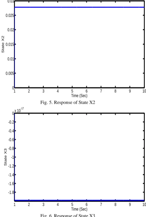
Fig. 5. Response of State X2
Fig. 6. Response of State X3
By considering the initial states of the system as zero if we plot the states of the system then we can get the Fig 4,Fig 5and Fig 6 and it can be seen that, state variable x1 is showing the same response as y as output y=x1 and other two states become stable after some time.
V. STATE FEEDBACK CONTROLLER USING LQR
Desired plant specifications which needs to be met by designing a controller, are first cast into a specific index or cost function, and the control is sought to minimize the cost function. This cost function can be minimized by designing a state feedback controller for various values of the optimal control and cost minimizing parameters like Q and R.
Let the system is defined by
x(t) =Ax(t) + Bu(t), x(0) ≠ 0, y(t) = Cx(t)
And the objective is to bring non zero initial state to zero. The cost function is scalar and it is defined by.
∫ (11) The Weighting matrices Q and R are symmetric and appear most often in the diagonal form. In addition, it is assumed that Q is semi-positive and R is positive. The optimal control has the form of state feedback u=-Kx.
1 2 3 4 5 6 7 8 9 10
0 100 200 300 400 500 600 700 800
Time (Sec)
Y
1 2 3 4 5 6 7 8 9 10
0 100 200 300 400 500 600 700 800
Time (Sec)
St
at
e
X1
1 2 3 4 5 6 7 8 9 10
0 0.005 0.01 0.015 0.02 0.025 0.03
Time (Sec)
St
at
e
X2
1 2 3 4 5 6 7 8 9 10
-1.8 -1.6 -1.4 -1.2 -1 -0.8 -0.6 -0.4 -0.2
0x 10 -17
Time (Sec)
St
at
e
The algebraic Recatti equation is given by
(12)
Where P is nxn symmetric matrix and
(13)
The LQR problem basically is the trade of where we give less weightage to the undesirable parameters and high weightage to the desired ones. Usually Q and R are selected to be diagonal so that specific state and control variables are penalized individually with higher weightings if their response is undesirable. In this case we will choose Q and R as follows, and use LQR method to get the feedback gain K, and make simulation under zero input situations. As it is single input and single output system so we set the initial condition as
x=[ ].
Matlab has a function named as 'lqr' which implements the above algorithm and returns the Eigen values, P and Gain matrix. When Q=[1 0 0; 0 1 0; 0 0 1] and R =1;
K = 1.0000 0.2379 0.0917 P =
36.2379 8.0917 1.0000 8.0917 4.2263 0.2379 1.0000 0.2379 0.0917 E =
-0.0278 -4.0320 + 4.4449i -4.0320 - 4.4449i
As it can be seen clearly from this result that Eigen values are all have negative real parts, so the closed loop system becomes stable, initially it was marginally stable as checked using pole zero map command.
Fig. 7. Output of the system with LQR Controller
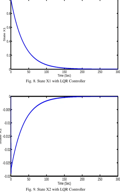
Fig. 8. State X1 with LQR Controller
Fig. 9. State X2 with LQR Controller
Fig. 10. State X3 with LQR Controller
0 50 100 150 200 250 300
0 0.2 0.4 0.6 0.8 1
Time (Sec)
Y
0 50 100 150 200 250 300
0 0.2 0.4 0.6 0.8 1
Time (Sec)
St
at
e
X1
0 50 100 150 200 250 300
-0.03 -0.025 -0.02 -0.015 -0.01 -0.005 0
Time (Sec)
St
at
e
X2
0 50 100 150 200 250 300
-0.08 -0.07 -0.06 -0.05 -0.04 -0.03 -0.02 -0.01 0 0.01
Time (Sec)
St
at
e
Fig. 11. Control Signal of LQR Controller
It can be seen that from Fig # 7, 8,9,10 it is clear that output and states reaches to steady state value after some time. Now let's define a general Q matrix as [ q 0 0; 0 q 0; 0 0 q] and change the value of q as 5,10 and 15 and make R=1 as constant and observe the results.
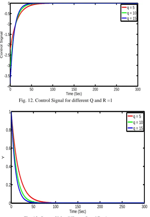
Fig. 12. Control Signal for different Q and R =1
Fig. 13. Output Y for different Q and R =1
Fig. 14. State X1 for different Q and R =1
Fig. 15. State X2 for different Q and R =1
Fig. 16. State X3 for different Q and R =1
From above figures it is clear that when we increase the value of q then the system approaches to zero more quickly and steady state error also reaches to zero very quickly. This is because we are increasing the weights for the states and making the weight constant for control signal. Therefore whatever the control signal the response is
0 50 100 150 200 250 300
-1 -0.8 -0.6 -0.4 -0.2 0
Time (Sec)
C
ont
rol
Sign
al
0 50 100 150 200 250 300
-4 -3.5 -3 -2.5 -2 -1.5 -1 -0.5 0
Time (Sec)
C
ont
rol
Sign
al
q = 5 q = 10 q = 15
0 50 100 150 200 250 300
0 0.2 0.4 0.6 0.8 1
Time (Sec)
Y
q = 5 q = 10 q = 15
0 50 100 150 200 250 300
0 0.2 0.4 0.6 0.8 1
Time (Sec)
St
at
e
X1
q = 5 q = 10 q = 15
0 50 100 150 200 250 300
-0.12 -0.1 -0.08 -0.06 -0.04 -0.02 0
Time (Sec)
St
at
e
X2
q = 5 q = 10 q = 15
0 50 100 150 200 250 300
-0.3 -0.25 -0.2 -0.15 -0.1 -0.05 0 0.05
Time (Sec)
St
at
e
X3
becoming faster. If we look at the control signal plot in Fig # 12, we can see that control signal size is little increasing with the increase of the Q since we are not increasing the weight R.
Now we keep q constant i.e. 1 and change the value of R and see the responses.
Fig. 17. Control Signal for different R and q =1
Fig. 18. Output Y for different R and q =1
Fig. 19. State X1 for different R and q =1
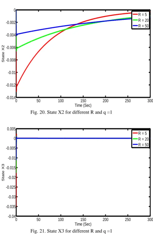
Fig. 20. State X2 for different R and q =1
Fig. 21. State X3 for different R and q =1
From figures it is quite clear that as we increase the value of R then output and states reaches to zero slowly and steady state error also reaches to zero very slowly. This is because we are increasing the weight for the control signal, so the control effort becomes smaller; therefore it takes more time for the output/states to reach the steady-state. If we look at the control signal plot in Fig # 17, we can see that control signal size is decreasing with the increase of the R.
VI. CONCLUSION
From the specified model of the plant, state space model was derived. Then its dynamic characteristics were studied. Then State Feedback controller was designed using LQR. It was found that when we increase the value of Q then system reaches to steady state more abruptly and when we increase the value of R then the system reaches to steady state slowly so state feedback controller was successfully designed for the system and the effects of Q and R were observed for the stability of the system.
0 50 100 150 200 250 300
-0.45 -0.4 -0.35 -0.3 -0.25 -0.2 -0.15 -0.1 -0.05 0
Time (Sec)
C
ont
rol
Sign
al
R = 5 R = 20 R = 50
0 50 100 150 200 250 300
0 0.2 0.4 0.6 0.8 1
Time (Sec)
Y
R = 5 R = 20 R = 50
0 50 100 150 200 250 300
0 0.2 0.4 0.6 0.8 1
Time (Sec)
St
at
e
X1
R = 5 R = 20 R = 50
0 50 100 150 200 250 300
-0.014 -0.012 -0.01 -0.008 -0.006 -0.004 -0.002 0
Time (Sec)
St
at
e
X2
R = 5 R = 20 R = 50
0 50 100 150 200 250 300
-0.04 -0.035 -0.03 -0.025 -0.02 -0.015 -0.01 -0.005 0 0.005
Time (Sec)
St
at
e
X3
REFERANCES
[1] W. J. Rugh., Linear System Theory, Prentice-Hall, Inc, 1996. [2] K. Ogata, Modern control Engineering, Pearson Prentice Hall.
[3] J. Douglas and M. Athans, "Robust LQR Control for the Benchmark Problem," in American Control Conference,.
[4] R. Datko, "The LQR Problem for Functional Differential Equations," in American Control Conference.
[5] E. Jones, "On the existence of optimal stabilizing controls," in Automatic Control, IEEE Transactions.
[6] N. N. a. P. V. D. J. Kautsky, "Robust pole assignment in linear state feedback".
[7] S. G. a. M. S. G.C. Goodwin, Control System design, Prentice Hall, 2011.
[8] J. Bay, Fundamentals of Linear State Space Systems, McGraw-Hill, 1999.
[9] J. Maciejowski, Multivariable Feedback Design, Addison-Wesley Publishing Company, 1991.
[10] B. A. a. J. Moore, Optimal Control. Linear quadratic method, Prentice-Hall International, 1989.