Manuscript Title & Authors

e-ISSN: 2278-7461, p-ISSN: 2319-6491

Volume 6, Issue 11 [November. 2017] PP: 50-55

Bivariate Weibull Chi-squaremodel based on Gaussian copula

MervetKhalifahAbd Elaal

1_{King Abdulaziz University Department of Statistics, Jeddah, Saudi Arabia} 2_{Al-Azhar University, Department of Statistics, Cairo, Egypt}

Abstract:

Key words:

Weibull Chi-square distribution; Bivariate Weibull Chi square distribution; Maximum likelihood

---Date of Submission: 04-12-2017 ---Date of acceptance: 16-12-2017

---I. Introduction

Recently, there has been an increased interest in defining ne w generators for univariate continuous families o f distributions b y introducing one or more additional shape parameter(s) to the baseline distribution. For instance, Cordeiro, et al. [4],Bourguignon et al. [3] proposed a generator of distributions called the Weibull -Gclass, Nadarajahet al.[8], and among others. The class of Weibull G distributions (WG) has received an increasing amount of attention in recent years. Many studiesconducted based on the properties and inferences of Weibull G distributions with a consideration to their applications. In this paper, we introduce a bivariate Weibull Chi-square distribution in the dependence structure and illustrate its applicability.

The(WG) probability density function (PDF) has the following

𝑓 𝑡, 𝛼, 𝛽, 𝛿 = 𝛼

𝛽𝛼 𝑔(𝑡,𝛿) 1−𝐺(𝑡,𝛿 ) −

𝑙𝑜𝑔 1−𝐺(𝑡,𝛿) 𝛽

𝛼 −1

𝑒𝑥𝑝 − −𝑙𝑜𝑔 1−𝐺(𝑡,𝛿)

𝛽 𝛼

, 𝑡 ≥ 0 (1)

where𝐺 𝑡, 𝛿 and 𝑔(𝑡, 𝛿), are Cdfand PDFof any baseline distribution depends on a parameter vector 𝛿, t is in the range of g(t, 𝛿), β > 0 is the scale parameter and 𝛼> 0 is the shape parameter. The (WG) distributionfunction (Cdf)is given by

𝐹 𝑡, 𝛼, 𝛽, 𝛿 = 1 − 𝑒𝑥𝑝 −𝑙𝑜𝑔 1−𝐺 𝑡,𝛿

𝛽 𝛼

, 𝑡 ≥ 0 (2)

Various Class Weibull G distributions have been discussed such as Weibull Pareto distribution by Alzaatreh, et al. [2].Copulas are a general tool to construct multivariate distributions and measure the dependence structure between random variables. The paper of Abd elaal [1] provided several methods of constructing bivariate distributions with copula functions.The main aim of this article is to introduce bivariate Weibull C h i s q u a r e (BWCH) model based on the most used copula function named Gaussian copula with a suitable organization. The paper is organized as follows. Section 2presents the bivariateWeibull Chi-square (BWCH) model based on Gaussian copula function. The maximum likelihood estimates (MLEs) for the model parameters are demonstrated in Section 3. In Section 4, the flexibility of the model is explained. Finally, the performance of the suggested model using a simulation data is discussed Section 5.

II. Bivariate Weibull C h i - s q u a r e distribution based on Gaussian copula

S u p p o s e t h a t 𝑔 𝑡 i s C hi-s quare d i st rib ut io n . W e h a v e g ( t ; r ) = 2− 𝑟 2 Γ 𝑟₂ 𝑡

𝑟

2−1_{exp −}𝑡

2 , 𝑡, 𝛼, 𝛽, 𝑟 >

0, a n d G ( t ; r ) i s 1−Γ 𝑡,

𝑟 2

Γ 𝑟₂ , where Γ 𝑡, 𝑟 2 𝑖𝑠

𝑓 𝑡, 𝛼, 𝛽, 𝑟 = 𝛼 2−

𝑟 2 Γ (𝑟₂₎𝑡

𝑟

2−1exp −𝑡 2

𝛽𝛼 _{1 −}1−Γ(𝑡, 𝑟 2) Γ(𝑟₂)

−

𝑙𝑜𝑔 1 −1−Γ(𝑡,

𝑟 2) Γ(𝑟₂)

𝛽

𝛼−1

𝑒𝑥𝑝 − −

𝑙𝑜𝑔 1 −1−Γ(𝑡,

𝑟 2) Γ(𝑟₂)

𝛽

𝛼

,

0 < 𝑡 < 𝑟 < ∞, 𝛼, 𝛽, 𝑟 > 0. (3) And

𝐹 𝑡, 𝛼, 𝛽, 𝑟 = 1 − 𝑒𝑥𝑝 − −

𝑙𝑜𝑔 1−1−Γ(𝑡, 𝑟 2) Γ (𝑟₂₎ 𝛽

𝛼

, 𝑡, 𝛼, 𝛽, 𝑟 > 0, (4)

The density of t h e W C H d i s t r i b u t i o n can be right-skewed. This fact implies that the WCHa n d B W C H d i s t r i b u t i o n s can be very useful to fit different data sets with various shapes. Now, let 𝑇1 and 𝑇2 a r e

f o l l o w i n g W e i b u l l - C h i - s q u a r e ( W C H ) d i s t r i b u t i o n t h e n t h e bivariate W e i b u l l C h i -s q u a r e ( B W C H ) d i -s t r i b u t i o n w h i c h d e f i n e d a -s t he joint PDF of 𝑇1 and 𝑇2 based on Gaussiancopula

becomes

𝑓 𝑡1, 𝑡2, 𝛼, 𝛽, 𝑟

= 𝛼𝑗2

−𝑟𝑗₂ Γ (𝑟𝑗_{2 )}

𝑡𝑟𝑗2 −1exp −𝑡𝑗 2

𝛽𝑗 𝛼_𝑗

1 −1−Γ(𝑡𝑗,

𝑟𝑗 2) Γ(𝑟𝑗₂)

−

𝑙𝑜𝑔 1 −1−Γ(𝑡𝑗,

𝑟𝑗 2) Γ(𝑟𝑗₂)

𝛽𝑗

𝛼_𝑗−1

𝑒𝑥𝑝 − −

𝑙𝑜𝑔 1 −1−Γ(𝑡𝑗,

𝑟𝑗 2) Γ(𝑟𝑗₂)

𝛽𝑗

𝛼_𝑗 2

𝑗 =1

1

1−𝜌2(exp[ −𝜌

2 1−𝜌2 𝜌 𝑧12+ 𝑧22 − 2𝑧1 𝑧2 ]) , 𝑡𝑗, 𝛼𝑗, 𝛽𝑗, 𝑟𝑗 > 0 (5)

(a) (b)

Fig.3 BWCH based on Gaussian copula: (a) Contour plot and (b) PDF curve

III. Parameter Estimation

In this section, we provide the estimation of the unknown parameters of BWCH distribution. There are two approaches to fitting copula models; parametric and semi-parametric methods.

3.1 Parametric methods of estimation

There are two approaches to fitting BWCH models. One approach is to estimate the marginal and copula parameters separately. The second approach is to obtain the estimation of the marginal and copula parameter from the pseudo-observations separately names modified ML.

3.1.1 Maximum likelihood estimation (ML)

The log-likelihood function expressed as

𝑙𝑜𝑔 𝐿 = 𝑛𝑖=1[𝑙𝑜𝑔 𝑓1 𝑡1𝑖 + 𝑙𝑜𝑔 𝑓2 𝑡2𝑖 + 𝑙𝑜𝑔 𝑐(𝐹1 𝑡1𝑖 , 𝐹2 𝑡2𝑖 )](6)

The estimation of BWCH distribution parameters obtained by ML in two-steps. The first step is estimating the

parameters of marginal distribution 𝐹1 and 𝐹2 by MLE separately as

log 𝐿𝑗 = 𝑛𝑖=1log 𝑓𝑗 𝑡𝑗𝑖 , 𝑗 = 1,2. (7)

Then, estimating copula parameters by maximizing the copula density is;

By considering the first step with (WCH) distribution, the parameters of each marginal distribution are estimated using MLE method. Now, if𝑡1, … , 𝑡𝑛 is a random sample from WE(𝛼𝑗,𝛽𝑗,𝑟𝑗), then the log-likelihood

function 𝐿(𝛼𝑗, 𝛽𝑗, 𝑟𝑗)becomes

log 𝐿𝑗(𝑡𝑗, 𝛼𝑗, 𝛽𝑗, 𝑟𝑗) = 𝑛𝑙𝑜𝑔 𝛼𝑗 + 𝑙𝑜𝑔 2 −𝑟𝑗₂ Γ (𝑟𝑗_{2 )}𝑡

𝑟𝑗

2 −1exp −𝑡𝑗𝑖 2 𝑛

𝑖=1 − 𝑛𝛼𝑗𝑙𝑜𝑔 𝛽𝑗 − 𝑙𝑜𝑔 1 −

1−Γ(𝑡_𝑗𝑖,𝑟𝑗₂) Γ(𝑟𝑗₂) 𝑛

𝑖=1 +

𝑛𝛼𝑗−𝑛𝑙𝑜𝑔−𝑙𝑜𝑔 1−1 − Γ(𝑡𝑗𝑖𝑟𝑗2)Γ 𝑟𝑗2)𝛽𝑗−𝑖=1𝑛− 𝑙𝑜𝑔 1−1 − Γ(𝑡𝑗𝑖, 𝑟𝑗2)Γ 𝑟𝑗2)𝛽𝑗𝛼𝑗.(9)

𝜕 log 𝐿𝑗(𝑡𝑗, 𝛼𝑗, 𝛽𝑗, 𝑟𝑗)

𝜕𝛼𝑗

= 𝑛 𝛼𝑗

− 𝑛 𝑙𝑜𝑔 𝛽𝑗 + 𝑛 𝑙𝑜𝑔 −

𝑙𝑜𝑔 1 −1−Γ(𝑡𝑗𝑖,

𝑟𝑗 2) Γ(𝑟𝑗₂)

𝛽𝑗

= 0 (10)

𝜕 log 𝐿_𝑗(𝑡_𝑗𝑖,𝛼_𝑗,𝛽_𝑗,𝑟_𝑗) 𝜕𝛽_𝑗 =

−𝑛𝛼_𝑗 𝛽_𝑗 +

𝑛 𝛼_𝑗−1 2

𝛽_𝑗 + 𝛼𝑗 −

𝑙𝑜𝑔 1−1−Γ(𝑡𝑗𝑖 , 𝑟𝑗

2 ) Γ(𝑟𝑗_{2 )} 𝛽_𝑗

𝛼_𝑗

𝑛 𝑖=1

1

𝛽_𝑗𝛼 𝑗 +1= 0 . (11)

𝜕 log 𝐿𝑗(𝑡𝑗,𝛼𝑗,𝛽𝑗,𝑟𝑗) 𝜕𝑟_𝑗 =

𝜕 𝑙𝑜𝑔 2 −𝑟𝑗₂ Γ(𝑟𝑗_{2 )} 𝑡

𝑟𝑗

2 −1exp −𝑡𝑗𝑖₂ 𝑛

𝑖=1

𝜕𝑟_𝑗 −

𝜕 𝑙𝑜𝑔 1−1−Γ 𝑡𝑗𝑖 , 𝑟𝑗

2 Γ 𝑟𝑗₂ 𝑛

𝑖=1

𝜕𝑟_𝑗 +

𝑛 𝛼_𝑗−𝑛 𝜕 𝑙𝑜𝑔

−𝑙𝑜𝑔 1−1−Γ 𝑡𝑗𝑖 𝑟𝑗

2 Γ 𝑟𝑗₂ 𝛽 𝑗

𝜕𝑟_𝑗 +

𝜕

− 𝑙𝑜𝑔 1−1−Γ(𝑡𝑗𝑖 , 𝑟𝑗

2 ) Γ(𝑟𝑗_{2 )} 𝛽 𝑗

𝛼 𝑗

𝑛 𝑖=1

𝜕𝑟_𝑗 = 0 (12)

The solution of the system of nonlinear equations (10),(11) and (12)gives the MLE of 𝛼𝑗, 𝛽𝑗,and 𝑟𝑗.Then copula

density will estimated as given,

log 𝐿(𝜃) = 𝑙𝑜𝑔 𝑐 𝐹 𝑡1 1𝑖 , 𝐹 2 𝑡2𝑖 𝑛

𝑖=1

13

Where 𝐹 𝑡1 1 and , 𝐹 2 𝑡2 denote the ML estimates of the parameters from first step. The solution of the

nonlinear equation (13) gives the MLE of 𝜃.

3.1.2 Modified maximum likelihood estimation (MML)

We will propose a modified ML method to obtain the model parameters of BWCH as follows. Firstly, the parameter estimation of marginal distribution 𝐹1 and 𝐹2by MLE separately computed as log 𝐿𝑗 =

log 𝑓𝑗 𝑡𝑗𝑖 , 𝑗 = 1,2. 𝑛

𝑖=1

The solution of the system of nonlinear equations (10),(11) and (12)gives the MLE of 𝛼𝑗, 𝛽𝑗,and 𝑟𝑗.Secondly,

estimate copula parameters by maximizing the copula density as log 𝐿 𝜃 = 𝑛𝑖=1log⁡[𝑐𝜃(𝑈𝑖, 𝑉𝑖)](14)

Where 𝑈𝑖, Viare pseudo-observations computed

from Ui= 𝑅_1𝑖 𝑛+1=

𝑛

𝑛+1𝐹 1 (𝑡1𝑖), Vi= 𝑅_2𝑖 𝑛+1 =

𝑛

𝑛+1𝐹 1 (𝑡2𝑖), 𝑅1𝑖 , 𝑅2𝑖are respectively the ranks of 𝑡1𝑖, 𝑡2𝑖.It is

important to respect that the margins Cdf.s estimated parametrically from the first step.

3.2 Semi-parametric methods of estimation

This section presents the semiparametric methods to estimate the copula model parameter.

Methods-of-moments

Following Kojadinovic and Yan [7], let c be a bivariate random sample from Cdf 𝐶𝜃 [𝐹1(𝑡1 ), 𝐹2(𝑡2)], where F1 and F2 are continuous Cdf.s and 𝐶θ is an absolutely continuous copula such that 𝜃 ∈ 𝒪, where 𝒪 is an open

subset of 𝑅2_{. Furthermore, let 𝑅}

1, . . . , 𝑅𝑛 are the vectors of ranks associated with 𝑡1, . . . , 𝑡𝑛 unless otherwise

of a consistent estimator of a moment of the copula 𝐶θ. The two best-known moments, Spearman’s rho and

Kendall’s tau, are respectively given by

ρ θ = 12 _[0,1]2u vdCθ u, v − 3, (14)

and τ θ = 4 _[0,1]2Cθ u, v dCθ u, v − 1.(15)

Consistent estimators of these two moments can be expressed as

𝜌𝑛= 12

𝑛(𝑛+1)(𝑛−1) 𝑅𝑖,1𝑅𝑖,2− 3 𝑛+1 𝑛−1 𝑛

𝑖=1 , (16)

And𝜏𝑛= 4

𝑛(𝑛−1) 1[𝑡𝑖,1≤ 𝑡𝑗 ,1]1[𝑡𝑖,2≤ 𝑡𝑗 ,2] − 1 𝑛

𝑖=1 (17)

When the functions ρ and τ are one-to-one, consistent estimators of θ is given by

𝜃𝑛,𝜌 = 𝜌−1 𝜌𝑛 ,𝜃𝑛,𝜏= 𝜏−1 𝜏𝑛 .

It called inversion of Kendall's (itau) and inversion of Spearman's rho (irho) respectively. For more information, see Kojadinovic and Yan [7].

IV. Goodness of fit tests for copula

The idea of this test is to compare the empirical copula with the parametric estimator derived under the null hypothesis seeDobrić and Schmid [5]. That is, test if C is well-represented by a specific copula 𝐶𝜃

𝐻0: 𝐶 = 𝐶𝜃𝑉𝑠. 𝐻1: 𝐶 ≠ 𝐶𝜃

Two approaches are commonly used in the literature to test the goodness of fit of a copula see Genest, et al.[6]. The goodness of fit tests based on the empirical process

ℂ𝑛 𝑢, 𝑣 = 𝑛 𝐶𝑛 𝑢, 𝑣 − 𝐶𝜃_𝑛 𝑢, 𝑣 ,

where𝐶𝑛 𝑢, 𝑣 is the empirical copula of the data of 𝑇1 and 𝑇2

𝐶𝑛 𝑢, 𝑣 =

1

𝑛 1 𝑈𝑖,𝑛 ≤ 𝑢, 𝑉𝑖,𝑛 ≤ 𝑣

𝑛

𝑖=1

, 𝑢, 𝑣 ∈ 0,1 ,

𝑈𝑖,𝑛, 𝑉𝑖,𝑛arepseudo observations from C calculated from data as follows. 𝑈𝑖,𝑛 = 𝑅_1𝑖

𝑛+1, 𝑉𝑖,𝑛 = 𝑅_2𝑖

𝑛+1, 𝑅1𝑖 , 𝑅2𝑖are

respectively the ranks of 𝑡1𝑖, 𝑡2𝑖.Here 𝐶𝑛 𝑢, 𝑣 is a consistent estimator and 𝜃𝑛 is an estimator of 𝜃 obtained

using the pseudo observations. According to Genest et al.[6], and Kojadinovic et al., [7], the test statistics is the

Cramer-von Miss and is defined as𝑆𝑛 = 𝐶𝑛 𝑈𝑖,𝑛, 𝑉𝑖,𝑛 − 𝐶𝜃_𝑛 𝑈𝑖,𝑛, 𝑉𝑖,𝑛 2 𝑛

𝑖=1

V. Simulation Data

In this section, a new bivariate proposed BWCH model based on Gaussian copula is presented. The correlation measures Kendall's tau and Spearman's rho of two variables with BWCH distribution are obtained and used to provide the values of copula parameter. Considering the following values of marginal and copula parametersof BWCH distribution based on Gaussian copulawith different sizes of sample (n = 30, 50, 100, and 150), where Gaussian copula parameterθ𝐺= 0.8.The estimations of parameters for the model by Gaussian

copula and the corresponding bias, mean squared errors and relative mean squared errors based on 1000 replications are reported in Table 1, 2, and 3.

To sum up, we observe the follows.

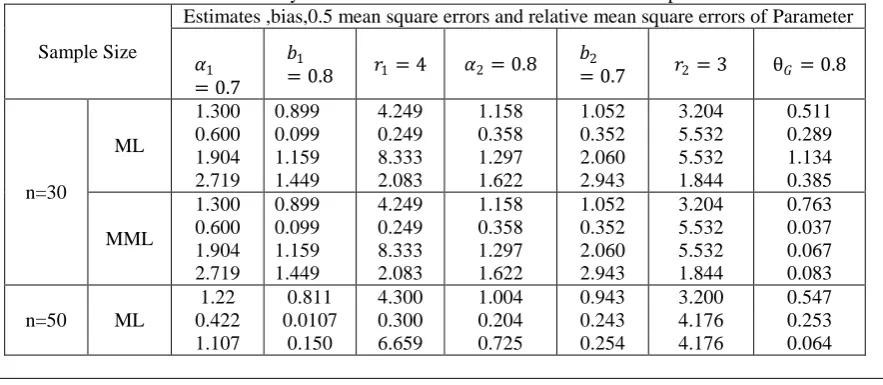
Table 1. The estimates, the bias, the mean squared errors and the relative mean squared errors of parameters by simulation study for BWCH distribution based on Gaussian copula

Sample Size

Estimates ,bias,0.5 mean square errors and relative mean square errors of Parameter

𝛼1

= 0.7 𝑏1

= 0.8 𝑟1= 4 𝛼2= 0.8 𝑏2

= 0.7 𝑟2= 3 θ𝐺 = 0.8

n=30

ML

1.300 0.600 1.904 2.719

0.899 0.099 1.159 1.449

4.249 0.249 8.333 2.083

1.158 0.358 1.297 1.622

1.052 0.352 2.060 2.943

3.204 5.532 5.532 1.844

0.511 0.289 1.134 0.385

MML

1.300 0.600 1.904 2.719

0.899 0.099 1.159 1.449

4.249 0.249 8.333 2.083

1.158 0.358 1.297 1.622

1.052 0.352 2.060 2.943

3.204 5.532 5.532 1.844

0.763 0.037 0.067 0.083

n=50 ML

1.22 0.422 1.107

0.811 0.0107

0.150

4.300 0.300 6.659

1.004 0.204 0.725

0.943 0.243 0.254

3.200 4.176 4.176

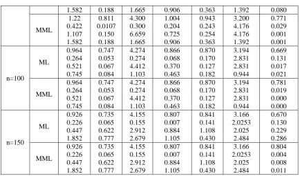
1.582 0.188 1.665 0.906 0.363 1.392 0.080 MML 1.22 0.422 1.107 1.582 0.811 0.0107 0.150 0.188 4.300 0.300 6.659 1.665 1.004 0.204 0.725 0.906 0.943 0.243 0.254 0.363 3.200 4.176 4.176 1.392 0.771 0.029 0.001 0.001 n=100 ML 0.964 0.264 0.521 0.745 0.747 0.053 0.067 0.084 4.274 0.274 4.412 1.103 0.866 0.068 0.370 0.463 0.870 0.170 0.127 0.182 3.194 2.831 2.831 0.944 0.669 0.131 0.017 0.021 MML 0.964 0.264 0.521 0.745 0.747 0.053 0.067 0.084 4.274 0.274 4.412 1.103 0.866 0.068 0.370 0.463 0.870 0.170 0.127 0.182 3.194 2.831 2.831 0.944 0.781 0.019 0.000 0.000 n=150 ML 0.926 0.226 0.447 1.852 0.735 0.065 0.622 0.777 4.155 0.155 2.912 2.679 0.807 0.007 0.884 1.105 0.841 0.141 1.108 0.430 3.166 2.0253 2.025 2.484 0.670 0.130 0.229 0.286 MML 0.926 0.226 0.447 1.852 0.735 0.065 0.622 0.777 4.155 0.155 2.912 2.679 0.807 0.007 0.884 1.105 0.841 0.141 1.108 0.430 3.166 2.0253 2.025 2.484 0.804 0.004 0.008 0.011

Table 2. The estimates, the bias, the mean squared errors and the relative mean squared errors of correlation parameter by simulation study for BWCH distribution based on Gaussian copula

Sample Size θ𝐺 = 0.8

Estimates

bias 𝑀𝑆𝐸 RMSE Method Estimation

n=30 0.511 0.763 0.796 0.797 0.289 0.037 0.004 0.003 1.134 0.067 0.010 0.022 0.385 0.083 0.013 0.007 ML MML Itau IRho n=50 0.547 0.771 0.755 0.762 0.253 0.029 0.045 0.038 0.064 0.001 0.002 0.001 0.080 0.001 0.003 0.002 ML MML Itau IRho n=100 0.669 0.781 0.777 0.776 0.131 0.019 0.023 0.024 0.017 0.000 0.001 0.001 0.021 0.000 0.001 0.001 ML MML Itau IRho n=150 0.670 0.804 0.806 0.804 0.130 0.004 0.006 0.004 0.229 0.008 0.021 0.012 0.286 0.011 0.026 0.015 ML MML Itau IRho

1. As expected, most results improve with increasing in sample size.

2. For most selected values of 𝛼1, 𝑏1, 𝑟1, 𝛼2, 𝑏2, 𝑟2 and 𝜃𝐺 the bias, MSE and RMSE of the estimates 𝛼 1, 𝑏 1,

𝑟 1, 𝛼 2, 𝑏 2, 𝑟 2 and 𝜃 𝐺 become smaller as the sample size increased.

3. the efficient estimators of marginal parameters of the model differ according to the parameters. It seems that ML estimates𝛼 1, 𝑏 1, 𝑟 1, 𝛼 2, 𝑏 2, 𝑟 2 and of the model are the same corresponding MML estimates.

4. For copula parameter, the MML provided efficient most estimates for the model with the marginals and Gaussian, copula parameters compared to ML, Itau, and Irho.

www.ijeijournal.com Page | 55 signficant p-value obtained using parmetric bootstrap for Gaussian copula function which indicate that selected parmetric copula function provide approporiate fit to the marginals. In addition, estimate of the copula parmeter based on ML, MML, Itau, and Irho methods for the Gaussian copula.This estimates are used as intial value when fitting this copula model using WCH marginals.

Table 3. Goodness of fit test statistics with their p-values and estimate of the copula parameter for selected copula functions.

model statistic p-value Estimate of copula

parameter

𝜃

Method estimation

BWCH 0.0235 0.3272 0.7949 Ml

0.0235 0.3422 0.7949 MML

0.0270 0.2792 0.7548 Itau

0.0261 0.3651 0.7625 Irho

Acknowledgments

The author would like to thank the Editor-in-Chief, and the referee for constructive comments, which greatly improved the paper.

References

[1]. Abd Elaal, M. K. (2017).Bivariate beta exponential distributions based on copulas. InternationalOrganization of Scientific ResearchJournal of Mathematics,13(3), 7–19.doi: 10.9790/5728-1303010719.

[2]. Alzaatreh A, Famoye F, Lee C (2013).Weibull-Pareto Distribution and Its Applications Communications in Statistics–Theory and Methods,42(9),1673–1691. doi:10.1080/ 03610926.2011.599002.

[3]. Bourguignon, M., Silva, R.B. and Cordeiro, G.M. (2014).The Weibull–G family of probability distributions, Journal of Data Science 12, 53–68.

[4]. Cordeiro, G.M. and de Castro, M. (2011).A new family of generalized distributions, Journal of Statistical Computation and Simulation 81, 883–893.

[5]. Dobrić, J., and Schmid, F. (2007).A goodness of fit test for copulas based on Rosenblatt’s transformation.Computational Statistics and Data Analysis, 51(9), 4633–4642. http://doi.org/10.1016/j.csda.2006.08.012

[6]. Genest, C., Rémillard, B., & Beaudoin, D. (2009). Goodness-of-fit tests for copulas: A review and a power study. Insurance: Mathematics and Economics, 44(2), 199–213.

[7]. Kojadinovic, I., and Yan, J. (2010). Comparison of three semiparametric methods for estimating dependence parameters in copula models, Insurance: Mathematics and Economics,47( 1), 52–63.

[8]. Nadarajah, S., and Rocha, R. (2016).Newdistns: An R Package for New Families of Distributions, Journal of Statistical Software, 69(10), 1-32, doi:10.18637/jss.v069.i10.