Abstract— Ozone is one of the most severe air pollution problems in the world. The concentration of ozone in the troposphere is of great interest because of its negative influence on the human health, vegetation and materials. The complexity of ozone (O3) formation mechanisms in the troposphere, the
complexity of meteorological conditions in urban areas and the uncertainty in the measurements of all the parameters involved, make fast and accurate modeling of ozone a challenging task. In the absence of a process model, multivariate statistical techniques, such as principal component analysis (PCA) have been successfully used in fault detection (FD) of highly correlated process variables. This paper presents an application of PCA in detecting abnormalities in ozone measurements, which are caused by air pollution or any incoherence between the different network sensors or sensor faults. Practical data from various ozone surveillance network stations in Upper Normandy, France, are used in this analysis.
Index Term— Ozone pollution, fault detection, principal component analysis.
I. INTRODUCTION
Air pollution has become a major concern in highly urbanized regions. Bad air quality negatively affects the public health, animals, plants, and the environment. People's health can be seriously affected by exposure to intense air pollution. This effect varies depending on the concentrations of the pollutants and the duration of exposure. In France as well as abroad, the study of air quality has attracted the attention of several researchers for a better understanding of the phenomenon of pollution and fight against atmospheric pollution [1]. Today, air quality is a multidisciplinary issue that involves both the epidemiological experts, transportation modeling specialists, specialists in transmission and transformation of pollutants,
T he authors gratefully acknowledge financial support from T exas A&M university at Qatar.
Fouzi Harrou , Chemical Engineering Program, T exas A&M University at Qatar,Doha, Qatar; (e-mail: Fouzi.harrou@
Qatar.tamu.edu).
Mohamed N. Nounou, Chemical Engineering Program, T exas A&M University at Qatar,Doha, Qatar; Corresponding author. T el.: +974 4423 0208; fax: +974 4423 0065., [email protected].
Hazem N. Nounou, Electrical and Computer Engineering Program, T exas A&M University at Qatar, Doha, Qatar,
specialists in geographic and diagnosis sys tems, local authorities and industry.
The impact of atmospheric pollution on human health is now at the forefront of population concerns [2]. Numerous epidemiological studies highlight the influence on the health of certain pollutants such as sulfur dioxide (SO2), nitrogen dioxide (NO2), ozone (O3) or dust particle in the air. The influence of this pollution is noticeable on sensitive populations , such as asthmatics, children, and elderly [3]. Currently, among the monitored atmospheric pollutants, ozone is one of the greatest concerns. Ozone is one of the most important photochemical oxidant that exerts adverse effects on human health as well as damages ecosystems, agricultural crops and materials at certain concentration levels [4-6]. France, like most European countries, has often known during the last summer seasons (2003 especially) episodes of ozone pollution, affecting a large part of the territory [7]. Therefore, monitoring the ozone pollution levels should be urgently considered in order to protect human health and environment.
The acceptable concentrations of various air pollutants are defined by European standards. Air quality monitoring networks have the following main missions: the measurement network management (i.e., recording of pollutant concentrations and the ranges of meteorological parameters related to pollution events), and the diffusion of data and information to the population and public authorities to warn against any dangers . The objective of this work is to propose a statistical detection method that can detect abnormal ozone measurements caused by air pollution or any incoherencies between the different network sensors or any sensor malfunctions. The developed detection method will be applied to ozone data obtained in the Upper Normandy region in France.
The complexity of ozone (O3) formation mechanisms in the troposphere [8], the complexity of meteorological conditions in urban areas and the uncertainty in the measurements of all the parameters involved, make the fast and accurate modeling of O3 very difficult. To overcome this difficulty, principal component analysis (PCA), which is a well-known multivariate data analysis technique, can be used it requires no prior knowledge about the process model [9]. PCA is one of the most popular multivariate statistical technique used to extract information from measured data and is widely used by scientists and engineers in various disciplines, such as in face
Statistical Detection of Abnormal Ozone Levels
Using Principal Component Analysis
recognition, data compression, image analysis, visualization, as well as in fault detection [10-12]. In the absence of a process model, PCA has been successfully used as a data-based FD technique for highly correlated process variables [10-12]. Due to its simplicity and efficiency in processing huge amount s of process data, it is recognized as a powerful tool in statistical process monitoring [13-16].
The remainder of this paper is organized as follows. Section II briefly presents the state of the art on ozone pollution and brief descriptions of the ozone data used in this work. Then, PCA is briefly introduced in Section III, and a description of how it can be used in fault detection is presented in Section IV. In Section V, we present the application of the PCA method to detect abnormal ozone measurements obtained from an air quality monitoring network in Upper Normandy, France. Finally, conclusions and future directions are presented in Section VI.
II. OZONE POLLUT ION
Generally, two types of ozone are distinguished . The first type of ozone is the stratospheric or good ozone, which is present at around 13 to 30 kilometers of altitude, and acts as a natural filter that protects life on earth from the harmful (ultraviolet) rays of the sun [17]. The ozone hole, which is a partial disappearance of this filter, is linked to the ozone destroying effects of certain pollutants emitted into the troposphere that move slowly into the stratosphere. The second type of ozone is the tropospheric ozone (often termed
bad ozone) or ground-level ozone. It is present in the air we breathe, and it causes eye irritation, bronchial, and can cause respiratory problems or asthma, especially among vulnerable persons (children, elderly) [2, 17]. The tropospheric ozone (O3) is a pollutant that has attracted growing interest in recent years [18, 19]. Unlike other pollutants , ozone is not directly emitted to the atmosphere. It is a called a secondary pollutant because it is formed as a result of complex chemical reactions involving two large families of pollutants known as primary pollutants, which are volatile organic compounds (VOC) and industrial emissions, which include nitrogen oxides (NOx) [17, 20]. The tropospheric ozone is formed gradually under the action of solar radiation, where NOx and VOC react chemically with oxygen to form ozone during sunny periods. That’s why ozone levels peak during the summer time.
A. Anomalies in ozone measurements
Two types of anomalies in ozone measurements (atypical ozone peaks) can be distinguished: true and false anomalies. The formation of a true anomaly of ozone requires certain conditions, which include s unny days under stagnant and humid air conditions , high humidity and high temperatures , and low wind speeds. These anomalies are large, with durations of several hours due to the long reaction time necessary for a gradual formation of the photochemical (tropospheric) ozone.
False anomaly, on the other hand, can be usually observed outside the summer times, where ozone concentrations abruptly increase to be in the range of 150.g/m3 to
3
/ .
600g m for short periods of time (around an hour). These abnormal measurements are sharply pointed, which are different from those observed in the case of photochemical ozone. The appearance of this type of anomalies may be due to different phenomena: a) possibility of a sensor malfunction, b) transported ozone produced elsewhere in the region, c) the possibility of stratospheric ozone intrusion into the low troposphere, and others [21].
The aim of this study is to use PCA to detect abnormal ozone measurements, both of anthropogenic origin (pollution peaks caused by human activity) or those encountered as a result of malfunctioning sensors. This application will be performed using ozone measurements obtained in the Upper Normandy region in France. More details about these data are provided in Section V. Since PCA is used in this application, a brief introduction to PCA, and a description of how it can be used in fault detection are presented next.
III. PRINCIPALCOM PONENTANALYSIS(PCA)
PCA is a linear dimensionality reduction modeling method, which can be helpful when handling data with a high degree of cross correlation among the variables. The main idea behind PCA is briefly introduced in this section, and more details can be found in [22, 27]. Let us consider the following data matrix
n m
X
consisting of n observations and m variables,1 2
[
T,
T,
,
T Tm]
X
x
x
x
, wherex
i
m. Before computingthe PCA model, the data matrix
X
is usually pre-processed by scaling every variable to have a zero mean and unit variance. This is because variables are measured with various means and standard deviations in different units. This preprocessing step puts all variables on an equal basis for analysis [23]. The data matrix X can be expressed using singular value decomposition (SVD) as follows:
X
TP
T (1)where,
T
[ , ,
t t
1 2
,
t
m]
n m is a matrix of thetransformed variables,
t
i
n, which are called the scorevectors or principal components, and
1 2
[
,
,
,
m]
m mP
p p
p
R
is a matrix of orthogonalvectors
p
i
m (also known as the loading vectors) whichare the eigenvectors associated with the covariance matrix of
X
, i.e.,Σ
. The covariance matrix,Σ
, is defined as follows:1
1
T T
X X
P P
n
Σ
(2)where,
PP
T
P P
T
I
n,
diag
(
1,
,
m)
is aorder
(
1
2
m)
, andI
n is the identity matrix[24].
Note that the PCA model results in the same number of principal components as the number of originals variables , m. In the case of collinear process variables, however, a smaller number of principal components (l) are needed to capture most of the variations in the data. Often, a small subset of the principal components (corresponding to the largest eigenvalues) can extract most of the important information in a data set, and thus simplify its analysis.
A. How many principal components to use?
The goodness of the PCA model depends on a good choice of how many principal components (PCs) to retain. Underestimating the number of PCs can leave out important variations in the data which degrades the prediction quality of the PCA model. Overestimating the number of PCs, on the other hand, introduces noise that masks the important features in the data. Thus, it is important to make a good estimate of the retained number of PCs. Several techniques for determining the number of PCs have been developed. The Scree plot [25] is one graphical technique, which plots the eigenvalues in a descending order and looks for a 'big gap' or an 'elbow' in the graph to determine the cutoff. Another technique is the cumulative percent variance (CPV), in which the smallest number of PCs that capture a certain percentage of the total variance (e.g., 90%) is chosen. The CPV is defined as follows:
100
)
(
)
(
1
trace
l
CPV
li
i .Cross validation is another popular criterion for choosing the number of PCs [26], which is based on minimizing a quantity, called PRESS that presents the sum of squared errors between the observed data and the approximated data. Other approaches include the parallel analys is, sequential tests, resampling, and profile likelihood [25, 27].
Once the number of principal components (l) is determined, the data matrix
X
can be expressed as follows:
X
TP
[
T
ˆ
T
~
][
P
ˆ
P
~
]
T (4)where,
T
ˆ
nl andT
~
n(ml), are matrices containing the (l) retained principal components and the (m-l) ignored principal components, respectively, and the matricesl m
P
ˆ
andP
~
m(ml)are matrices containing the (l) retained eigenvectors and the (m-l) ignored eigenvectors, respectively. Expanding equation 4, we get:
X
T
ˆ
P
ˆ
T
T
~
P
~
T
X
ˆ
E
(5) where,T
P
P
X
X
ˆ
ˆ
ˆ
andE
X
(
I
m
P
ˆ
P
ˆ
T)
.IV. FAULTDETECTIONINDICES
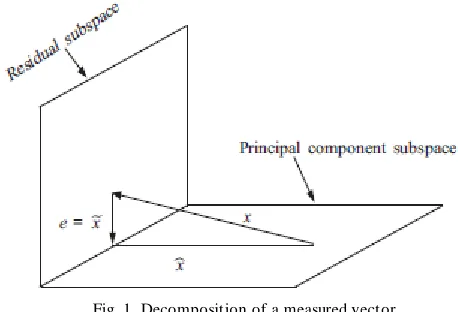
As shown in equation (5), a measured vector x can be expressed using PCA as the sum of two orthogonal parts,
approximated vector ˆx and residual vector x (see Fig. 1). The residual vector x is usually small in a fault-free situation, but it can greatly increase in the presence of a fault.
Fig. 1. Decomposition of a measured vector.
In fault detection using PCA, a PCA model is constructed using fault-free data, and then the model is used to detect faults using one of the detection indices . One of commonly used detection indices is the
Q
statistic, which is describednext.
A. The
Q
statistic or squared prediction error (SPE)The
Q
statistic or Rao-statistic (also referred to as thesquared prediction error, SPE) measures the projection of a data sample on the residual subspace, which provides an overall measure of how a data sample fits the PCA model.
Q
is defined as the sum of squares of the residuals obtained from the PCA model, i.e., [10]:x
P
P
x
x
x
Q
~
T~
T~
~
T (7)where,
~
x
x
x
ˆ
(
I
P
ˆ
P
ˆ
T)
x
.
The monitored system is considered to be operating normally if:
Q
Q
(8)where, the value of the threshold
Q
is given by Jackson andMudholkar [17]:
2 1 0 0 2 1 2 0 1)
1
(
1
2
h
h
c
h
Q
(9)where,
,
1
,
2
,
3
1
mi
l j
i j
i
, 22 3 1 0
3
2
1
h
, wherel
is the number of retained PCs, andc
is the value of the normal distribution with
level of significance. This value of threshold is calculated based on the assumptions that the measurements are time-independent and multivariate normally distributed. TheQ
fault detection index is very sensitive toB. Fault detection using PCA
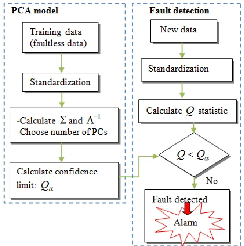
Fault detection using PCA involves the following steps (see Fig. 2): 1) the development of a statistical model from historical data collected when the process runs under normal operating conditions; 2) the determination of control limits for the statistical model (e.g., the
Q
statistic limits); and 3) the detection of process faults when new data exceeds the control limits.Fig. 2. A block diagram of the PCA fault detection algorithm.
V. RESULTS AND DISCUSSION
In this Section, PCA is used to monitor the ozone levels using real ozone data obtained in the Upper Normandy region , France. Descriptions of the ozone data and the region un der study are presented next.
A. Ozone data sets and study region
In this study, the Upper Normandy region in France was selected for data collection. Upper Normandy is located at northwest of Paris, near the south side of Manche sea and is one of the most highly industrialized areas in France. This city, like most large European cities, faces air pollution problems. Air Normand is the official association responsible for monitoring air quality in the Upper Normandy region, and for providing the public with information on any findings. The association consists of 7 stations placed in rural, peri-urban and urban sites, across the region.
The ozone data used in this application were measured each fifteen minutes in order to limit spatial and temporal sampling problems. Measured fault-free ozone data (collected between 11 August and 19 August, 2006, for a total of 773 observations) were used to develop a PCA reference model. Plots of these ozone measurements and their corresponding
auto-correlation functions (ACF) are shown in Fig.s 3a and 3b, respectively. Only the curves of the three stations SRC, QUI and ND2 are plotted for better readability of the fig.s. The data from the other stations have similar trends.
Fig. 3. (a) Quarter-hourly ozone concentrations in Upper Normandy, and (b) ACF of O3 concentrations.
Fig. 3b shows a clear periodicity of the ACF every 24 hours (period between adjacent peaks in the ACF). It is well known that the distance between extreme points in the autocorrelation functions gives the period of the time series. This periodic behavior is related to the diurnal cycle of ozone, which is primarily caused by the diurnal temperature cycle that affects the ozone levels. Fig. 3b also shows a similarity between the autocorrelation functions for all ozone measurements from all network stations. An advantage of PCA is that it can handle such a high dimensional data set having a high degree of correlation among the variables.
B. Ozone modeling using PCA
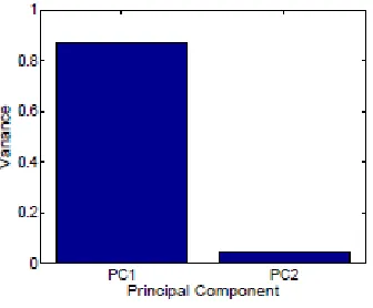
86.88 % and 4.34% of the total variations in the data, as shown in Fig. 4.
Fig. 4. Variance captured by each principal component.
The PCA based monitoring algorithm (described in Section IV) is first carried out using the training fault-free data. Based on the first two PCs, the
Q
statistic for the PCA algorithm is usedfor fault detection. The result of the
Q
statistic is shown inFig. 5, where the dotted line represents the detection threshold
Q
, which is found to be 1.439. Fig. 5 shows that theQ
statistic is always below the threshold which means that the data belong to the normal operating region.
Fig. 5. T he time evolution of the
Q
statistic on a semi-logarithmic scale for the fault -free data.C. PCA fault detection
In this subsection, the performance of the PCA fault detection scheme will be evaluated using real ozone testing data sets. Two ozone monitoring examples are presented in order to illustrate the performance of the PCA fault detection scheme in this ozone monitoring application. The first example involves a sensor fault (false anomaly) in station 'QUI'. In the second example, on the other hand, PCA is used in the detection of multiple faults.
a) Sensor anomaly detection: simple fault case
The PCA model developed using the fault-free data is used in this section to detect possible simple sensor faults using unseen testing data. The testing data set consists of 361 data samples, measured from 03 August to 7 August 2006, which are completely independent from the training data. In this case, the possibility of only a single fault (i.e., in one variable) is considered. This testing data contains an abnormal ozone
measurement. This fault occurs in station 'QUI' between sample numbers 289 and 290 (6 August 2006 at 05:00pm), with a maximum intensity level of
350
.
g
/
m
3. Fig. 6 which plots the value of theQ
statistic based on the testing data, shows that this fault is detected by exceeding the threshold value. However, Fig. 6 also shows that theQ
test resulted in somefalse alarms, which are indicated by the red crosses.
Fig. 6. T he time evolution of the
Q
statistic on a semi-logarithmic scale in the presence of a simple sensor fault.b) Abnormal ozone detection: multiple fault case
In this example, we verify the PCA model ability to detect multiple faults. The ozone concentrations data measured between 5-7 September 2006, consist of 200 data samples . In this data set, faults simultaneously occur in stations 'ND2' and 'TAN' from sample numbers 21 to 34 (which occur on September 5, from 07:45am to 11:00am), and in stations 'LIL', 'ND2' and 'GRV' from the sample numbers 119 to 146 ( on September 6, from 08:45am to 03:00pm). Fig. 7 shows that the
Q
test is capable of detecting all faults but on the expense of a lot more false alarms (which are indicated by the red crosses) than in the simple fault case. This is mainly due to the fact that PCA is a linear modeling technique, and is thus inappropriate to use it in modeling nonlinear processes. In the case of nonlinear data, such as the ozone data used in this application, this modeling error reflects on the effectiveness of the PCA-based fault detection algorithm.Fig. 7. T he time evolution of the
Q
statistic on a semi-logarithmic scale in the presence of multiple faults.VI. CONCLUSION
in different stations , were performed. The results show that PCA is capable of detecting single and multiple fault, but on the expense of many false alarms, especially for the multiple fault case. This is mainly due to the fact that PCA is a linear modeling technique, and thus does not suit the nonlinear nature of the ozone formation process . Therefore, building nonlinear PCA models is expected to reduce the rate of false alarms.
ACKNOWLEDGMENT
The authors gratefully acknowledge financial support from Texas A&M University at Qatar. The authors also would like to thank Air Normand which made available the atmospheric pollution data used in this article.
REFERENCES
[1] L.Basly, T élédétection pour la qualité de l'air en milieu urbain, Ph.D. thesis, Sciences de technologies de l’information et de la communication, Université de Nice Sophia Antipolis, 2000. [2] H.Moshammer, “Communicating health impact of air pollution”,
Air Pollution, ed: Vanda Villanyi, Intech, 2010.
[3] E. Marchwinska-Wyrwal, G. Dziubanek, I. Hajok, M. Rusin, K.Oleksiuk and M.Kubasiak . “Impact of Air Pollution on Public Health”, in, T he Impact of Air Pollution on Healt h, Economy, Environment and Agricultural Sources, Mohamed K. Khallaf (Ed.), ISBN: 978-953-307-528-0, InTech, 2011.
[4] WHO, “ Health Aspects of Air Pollution”, World Health Organization, 2004.
[5] Air pollution primer. National T uberculosis and Respiratory Disease Association, New York, 1971.
[6] I.F. Gheorghe and B. Ion, “T he Effects of Air Pollutants on Vegetation andthe Role of Vegetation in Reducing Atmospheric Pollution”, in T he Impact of Air Pollution on Health, Economy, Environment and Agricultural Sources, Mohamed K. Khallaf (Ed.), ISBN: 978-953-307-528-0, InT ech, 2011.
[7] M. Poumadere, C.Mays, S. Le Mer, and R. Blong, T he 2003 heat wave in France: dangerous climate change here and now, Risk Analysis, 25(6), 1483-1494, 2005.
[8] J.H. Seinfeld and S.N. Pandis. “Atmospheric chemistry and physics: from air pollution to climate change”, John Wiley & Sons, Inc , New York, 2006.
[9] M. Kano and Y. Nakagawa. Data-based process monitoring, process control, and quality improvement: Recentdevelopments and applications in steel industry. Com puters & Chem ical Engineering, 32(1-2):1224, 2008.
[10]S.J. Qin. “Statistical process monitoring: Basics and beyond”,
Journal of Chem om etrics, 17(8/9):480–502, 2003.
[11]A. Herve and J.W. Lynne. “Principal component analysis”, Wiley Interdisciplinary Reviews: Com putational Statistics, 2:433–459, 2010.
[12]W. Li, H. Yue, S. Valle, and S.J Qin. “Recursive pca for adaptive process monitoring”, Journal of Process Control, 10:471–486, 2000.
[13]S.I.V. Sousa, F.G. Martins, M.C.M. Alvim-Ferraz, and M.C. Pereira. “Multiple linear regression and artificial neural networks based on principal components to predict ozone concentrations”. Environm ental Modelling & Software, 22:97–103, 2007.
[14] X.Sun, H.J. Marquez and T .Chen, An improved PCA method with application to boiler leak detection, ISA Transactions, 44(3), 379– 397, 2005.
[15]J.P. George, Z. Chen and P. Shaw, Fault Detection of Drinking Water T reatment Process Using PCA and Hotelling T2 Chart,
World Academ y of Science, Engineering and Technology, 50, 970-975, 2009.
[16]J. Yu, Fault Detection Using Principal Components-Based Gaussian Mixture Model for Semiconductor Manufacturing Processes, IEEE Transactions on Sem iconductor Manufacturing, 24(3), 471-486, 2011.
[17]S. Sillman. “T ropospheric ozone and photochemical smog”. in B. Sherwood Lollar, ed., T reatise on Geochemistry, Environm ental Geochem istry, Ch. 11, Elsevier, 9:407–431, 2003.
[18]Ch. Vlachokostas, S.A. Nastis, Ch. Achillas, K. Kalogeropoulos, I. Karmiris, N. Moussiopoulos, E. Chourdakis, G. Banias, and N. Limperi. “ Economic damages of ozone air pollution to crops using combined air quality and gis modeling”. Atm ospheric Environm ent, 44:3352–3361, 2010.
[19]A. Detournay, S. Le Meur, and V. Delmas. “Understanding of the atypical ozone peaks phenomenon observed around the petrochemical industrial zone of port -jerome in Upper Normandy, France”. Pollution atmosphrique, 196: 405–422, 2007.
[20]G.Brulfert, O.Galvez, F.Yang and J.J.Sloan, “A regional modelling study of the high ozone episode of June 2001 in southern Ontari”,
Atm ospheric Environm ent, 44, pp.3777-3788, 2007.
[21]I. Zdanevitch. “ Etude d’pisodes inexpliqus d’ozone”. Rapport LCSQA, convension 41/2000. INERIS, Paris., 2001.
[22]J.F. MacGregor and T . Kourti. “ Statistical process control of multivariate processes”. Control Engineering Practice, 3(3), 1995. [23]P. Ralston, G. DePuy, and J.H. Graham. “ Computer-based
monitoring and fault diagnosis: a chemical process case study ”. ISA Transactions, 40(1):85–98, 2001.
[24]J.E. Jackson and G. Mudholkar. “ Control procedures for residuals associated with principal component analysis”. Technom etrics, 21:341349, 1979.
[25]M. Zhu and A. Ghodsi. ’’Automatic dimensionality selection from the scree plot via the use of profile likelihood . Com putational Statistics & Data Analysis, 51:918–930, 2006.
[26]G. Diana and C. T ommasi. “ Cross-validation methods in principal component analysis: A comparison”, Statistical Methods & Applications, 11(1):71–82, 2002.
[27]I.T . Jolliffe. “Principal component analysis”. second edition,Springer, Berlin, 2002.
[28]A. Benaicha, M. Guerfel, N. Boughila, and K. Benothman.” New PCA-based methodology for sensor fault detection and localization”. In MOSIM’10, Hammamet, T unisia, May 10-12 2010.