Abstract— Standard approaches to evaluate the ground-state
properties of the Hubbard model via the Lanczos method have convergence problems upon the growing difference between hopping and Coulomb interaction strength. This issue is quite relevant since energy convergence does not necessarily translate into convergence of the ground-state itself. Here we discuss several algorithms such as the standard Lanczos method, Explicit Restarted Lanczos algorithm (ERL), and the Modified Explicit Restarted Lanczos algorithm (MERL), and introduce a protocol based on them, using the S2 operator as a stopping criterion, since it is possible to track the error in the ground-state evaluation. We find that the ERL-based algorithm provides a much better precision and it is 5 times faster when compared to the conventional one. The MERL-based algorithm keeps the error at the last significant digit and its processing time takes about 2.5 times longer than the ERL algorithm, although it is still faster than the standard Lanczos scheme. Our findings pave the way for a reliable and practical evaluation of the ground-state properties not only of the Hubbard model, but also for many other many-body quantum systems.
Index Term— Diagonalization, Hubbard model, Lanczos
Method, Quantum State Transitions.
I. INTRODUCTION
Critical phenomena stands as one the major fields in physics. It is important for the development and optimization of solid-state devices and provides a better understanding of complex statistical systems. The melting of ice or sudden changes in magnetic correlations of an iron bar, for instance, are phase transitions induced by temperature [1]. Critical behavior can also be found in quantum systems at absolute zero temperature. In this case, the ground state may face abrupt changes by varying a given physical parameter, and thus the phase transition is triggered due to quantum, instead of thermal, fluctuations. A paradigmatic example is the metal to insulator transition in the electronic Hubbard model [2-4], which is the framework we use in this paper. It emerges from the competition between electron hopping and the local coulomb potential. Other examples include superconducting transitions, in which the electrical resistance falls to zero, the Mott-insulator to superfluid transition in the bosonic version of the Hubbard model [5], and also in coupled cavity QED
*e-mail: [email protected]
systems [6], and many others (for a review see, e.g., Ref. [7]). These phenomena are simply known as a quantum phase transitions [8].
In particular, the Hubbard model is applied to study the behavior of strongly correlated electron systems. It describes a lattice of fixed sites where electrons can tunnel among next-neighbor sites at the same time it can locally interact with another electron via Coulomb repulsion or attraction. The Hamiltonian of the Hubbard model reads
i i i j
i
j i j
i
c
c
U
n
n
t
H
, ,,
, †
, ,
, (1)
where i and j represent the lattice sites,
denotes the spindirection,
c
i†, (c
i,) is the fermionic operator which creates(destroys) an electron with spin
at site i, following thestandard anticommutation rules for fermions, and
n
i,is thenumber operator. Here we take the hopping amplitude to be uniform along the lattice, ti,j = t.
The most straightforward numerical method to study those transitions is to simply diagonalise the corresponding Hamiltonian, thus finding its energy spectrum along with its eigenstates for a given set of parameters. However, it turns out to be computationally unattainable to deal with the exponentially increasing number of states when we add more sites and/or particles into the lattice. In addition, as long as the ground state, and its related quantum phase transition, is the only object of interest, it is useless, if not impossible to proceed with a robust evaluation of the whole spectrum. An alternative which requires much less resources is the Lanczos method [10]. Through a modified version of this protocol, it is possible to obtain only the ground state using iterations which do not take the other eigenstates into account [11,12].
In the Hubbard model, the Lanczos method is quite efficient when the two competing parameters, i.e., the hopping amplitude t and the Coulomb interaction strength U are of the same order of magnitude [13-16]. But in some studies should be necessary to analyse strong coupling systems, as the work made by Ribeiro in which the interaction parameter is three times the non-interacting energy bandwidth, U = 48t [17]. Then in some systems, where quantum state transition occurs in the strong coupling regime, the Lanczos method shows crucial convergence problems, even for simple systems. Here we show how to surpass this problem by presenting a protocol that ensures a precise result for the ground-state energy and
Efficient ground-state evaluation of the Hubbard
model using an approach of the Lanczos method
T. X. R. Souza
*and C. A. Macedo.
vector.
The remainder of this paper is organized as follows. In Sec. II, we introduce the standard Lanczos method. In Sec. III, we describe the quantum operator S2, which will be used as a new stopping criterion for the method. In Sec. IV, we implement the algorithms and, in Sec. V, we analyze the results comparing the processing times and precision rates. Conclusions are drawn in Sec. VI.
II. LANCZOS METHOD
In order to deal with the Hubbard model in finite lattice sizes, a diagonalization of its Hamiltonian, Eq. (1) is required. In grand-canonical systems, however, the size of the array grows exponentially with the number of sites, where the
Hilbert-space dimension is Dim H =
4
Ns. Since the Hubbard Hamiltonian preserves the number of particles and spin, it is possible to deal with separate manifolds, at which the number of states is given by
N
N
N
N
H
sub s sDim
, (2)thus greatly reducing computational cost. Another technique to reduce the memory allocation is write the Hamiltonian hopping matrix as a Kronecker sum, which is given by
H
H
H
I
I
H
H
hop , (3)where
is the Kronecker product,H
andI
are theHamiltonian and the identity operator for particles with spin
. In this form the Hamiltonian cam be storage as twosquared matrix with dimensions
N s Nand
N s N, and a
diagonal matrix with the interaction part of the Hamiltonian [16].
Standard diagonalization techniques aim for computing the whole eigenstate spectrum. However, our aim is to efficiently compute the ground state of the Hubbard model. Then, the Lanczos method arises as a great tool for this task, allocating as less memory as possible. This method consists in building a new set of orthogonal basis vectors for the system, so that the Hamiltonian matrix takes a tridiagonal form. This set of vectors is defined in a Krylov subspace. The algorithm starts
with a random initial vector
0 , from which a set oforthogonal vectors is spanned following the recurrence rule
1 2
1
n
n n
n nn
H
a
b
, (4)Where n n n n n
H
a
and1 1 2
n n n n nb
. (5)
The tridiagonal Hamiltonian matrix representation then takes the form
1 1 1 2 2 2 1 1 1 00
0
0
0
0
0
n n n Ta
b
b
a
b
b
a
b
b
a
H
. (6)
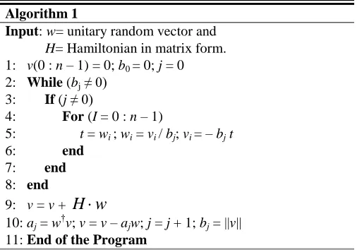
Now, the ground-state evaluation is done by using an iteration algorithm [18] obeying m < n, with n =Dim(H) as seen below in Algorithm 1, where v, w and a are vectors with
length n, and b is also a vector with length n – 1.
H
w
is the resulting product of H and w. a and b are, respectively, the main and secondary diagonal of matrix HT.Algorithm 1
Input: w= unitary random vector and
H= Hamiltonian in matrix form. 1: v(0 : n – 1) = 0; b0 = 0; j = 0
2: While (bj ≠ 0)
3: If (j ≠ 0)
4: For (I = 0 : n– 1)
5: t = wi ; wi = vi / bj; vi = – bj t
6: end
7: end
8: end
9: v = v +
H
w
10: aj = w†v; v = v – ajw; j = j + 1; bj = ||v||
11: End of the Program
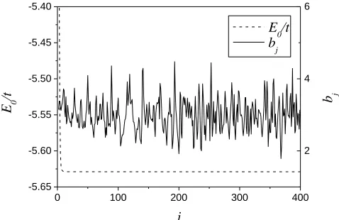
Due to numerical inaccuracies, it is well known that the vectors orthogonality is lost [19], and so the stopping criterion in line 2 of Algorithm 1 may never be reached, as shown in Fig. 1. The situation gets worse for higher j and thus one ends up with duplicated or wrong eigenvalues. This issue can be avoided by applying the Gram-Schmidt orthogonalization procedure, but it requires more processing time, as well as memory allocation, due to the large number of vectors involved. A way to overcome this problem is to include another stopping criterion at j < n, and so we now replace line 2 of Algorithm 1 with
While (bj ≠ 0 or j < m), (7)
this analysis for the case of a half-filling one-dimensional lattice with Ns = 6.
0 100 200 300 400
-5.65 -5.60 -5.55 -5.50 -5.45 -5.40
E
0/t
E0
/t
j
2 4 6
bj
b j
Fig. 1. Ground-state energy (dotted line) and bj (solid line) as a function of j. j is the number of Lanczos vectors created by the algorithm.
Setting a limit to the amount of Lanczos vectors that can be created is not a reliable step when the system's convergence point is unknown. Thus, it is possible to stop the iteration when the ground-state energy converges, i.e., when its precision fulfills the chosen error parameter. This is accomplished by diagonalizing H at each iteration. Then, let us include the following procedure after line 10 in Algorithm 1:
Diag(a, b, j|E0, V0)
Error = |E0 – E| , (8)
E = E0
where Diag(a, b, j|E0, V0) is the outcome for the tridiagonal
matrix, where the vector a is the main diagonal and b is the secondary diagonal. E0 and V0 are, respectively, the
ground-state eigenvalue and the eigenvector, the basis of V0 are the
Lanczos vectors generated. The stopping criterion shown at line 2 of Algorithm 1 must then be modified by
While (Error > X). (9)
Algorithm 1 must be used in situations where only the ground-state energy is needed, since it does not store all the system's eigenvectors. However, we have to precisely compute, at least, the ground state itself by retrieving the basis states. Algorithm 2 shows how the ground state can be accessed, where yj is the component j of the ground state
vector V0 and r denote, at the end of the process, the state
written in the conventional Hamiltonian basis.
Algorithms 1 and 2 allow obtaining both the ground-state energy and vector. These are enough for studying quantum state transitions in the Hubbard model. But as it was mentioned before, there is loss of orthogonality during the creation of vectors in the Lanczos method and this may affect the ground-state precision. What can be done is to restart the
Lanczos algorithm using a previous ground state, calculated with fixed m, as the initial vector. This scheme is known as the Explicit Restarted Lanczos (ERL) algorithm [20], at which successive rounds stops after the convergence of the ground state. In the following section we introduce the quantum operator that will be used as an additional stopping criterion in our algorithm.
Algorithm 2
Input: w= Same random vector of Algorithm 1.
a, b and m from Algorithm 1.
y= Ground state vector from Algorithm 1. 1: v(0 : n – 1) = 0
2: r(0 : n – 1) = 0 3: Forj = 0 : m - 1 4: If (j ≠ 0)
5: For (I = 0 : n– 1)
6: t = wi ; wi = vi / bj; vi = – bj t
7: end
8: end
9: r = r + yjw
10: v = v +
H
w
11: v = v–ajv12: end
13: End of the Program
III. TOTAL SPIN SQUARED (S2)
Obtaining eigenvalues using the Lanczos method is a quite simple, since it is made by analyzing the convergence of a single variable in the algorithm. However, the eigenvector analysis involves a large number of variables, about the order of the Hilbert-space dimension of the underlying Hamiltonian, which is often large, especially in Hubbard-like models.
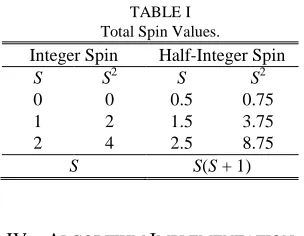
An indirect way to analyze the convergence of the eigenvector is through applying a quantum observable whose outcomes are previously known. Here, we introduce an algorithm that computes the S2 value for the ground-state vector r. We chose the S2 operator rather than other quantum operators since its possible values are simply given by
S2=S(S+1).
In the Hubbard model the spin ladder operators are
, †
, , †
, †
i i i
i i i
c
c
S
c
c
S
. (10)
Then the S2 operator is
}
2
)
2
,
(
{
4
1
, †
, , †
, , ,
, ,
2
i j j i j i
ij j
j i
c
c
c
c
n
n
n
S
. (11)
be defined and, although it is not possible to predetermine its exact value, the possible outcomes are listed in Table I.
TABLE I Total Spin Values. Integer Spin Half-Integer Spin
S S2 S S2
0 0 0.5 0.75
1 2 1.5 3.75
2 4 2.5 8.75
S S(S + 1)
IV. ALGORITHM IMPLEMENTATION
We now propose two algorithms to overcome the aforementioned convergence problems in the Lanczos method. Afterwards, it is possible to evaluate the ground-state properties of the Hubbard model in limiting interaction regimes.
The first is based on the ERL algorithm, at which a new stopping criterion was included. We use Algorithms 1 and 2 with fixed number of Lanczos vectors m. In each restart, the tridiagonal matrix is diagonalized yielding the ground-state vector and its corresponding energy. It then becomes the new input vector for another turn. This process goes on and on until both the energy and the S2 operator reach their convergence criteria. The second algorithm is based on the Modified Explicit Restarted Lanczos (MERL) algorithm [20]. It starts as the ERL scheme and, after reaching its convergence, another ERL iteration is triggered with a lower number of Lanczos vectors, as shown in Algorithm 3.
Algorithm 3
Input: Ns = Number of sites.
1: N = Ns
2: While (N > 2)
3: While (Error > X and S2error > Y ) 4: Do the Algorithm 1: With m = N
5: Do the Algorithm 2: With m = N
6: Diag(a, b, m|E0, V0)
7: Error = |E0–E|
8: E = E0
9: w = V0
10: If (Error > X) 11: S2value(V0|S2)
12: S2error = S2- Stest
13: Stest = S2
14: end
15: end
16: N = N– 4 17: end
18: End of the Program
The main concern during the development of this algorithm was to minimize the memory allocation due to the large number of states involved. In Hubbard-like models, one should deal with as minimum states as possible in order to be able to increase the size of the lattice. For instance, there is a growing interest in GPU parallel programming to deal with this kind of problem [16] and those devices have even less memory than conventional CPUs. Anyway, due to this memory limitation, we shall not use the MERL algorithm and so we will be dealing with single-precision variables only.
V. RESULTS Standard Lanczos Method
In order to analyse the algorithms presented so far, we use a quasi-one-dimensional ladder lattice with an open boundary condition. This simple structure need less concern about lattice frustrations and symmetries, making it an appropriate system to be used in computational tests. The number of electrons was fixed to Ne = Ns– 1 and the number of sites was Ns = 6, 8, and
10. We analyse the lowest Sz subspace in each case. Figures 2,
3 and 4 show the behavior of the ground-state energy and S2 as a function of the number of Lanczos vectors for U = 1t, U = 10t, and U = 80t (strong-coupling regime).
For weak and intermediate interaction strengths, the ground-state energy converges almost at the same point as S2. In this
scenario, the total spin remains 1/2 and the system does not go through a phase transition. However, in the strong-coupling regime, U=80t, the ground-state energy converges earlier than
S2, especially for larger lattices. For Ns = 6 and 8, there is a
0 10 20 30 40 50 -6.5
-6.0 -5.5 -5.0 -4.5
0 10 20 30 40 50 60 -9
-8 -7 -6 -5
0 20 40 60 80 100 -12
-10 -8 -6
Ns=6, Ne=5
E
0/t
S2
E
0/
t
j
(a)
U/t=
1
0.0 0.5 1.0 1.5 2.0
S
2
(b)
Ns=8, Ne=7
E0/t
S2
E
0/
t
j
0.0 0.5 1.0 1.5 2.0
S
2
(c)
Ns=10, Ne=9
E0/t
S2
E
0/
t
j
0.0 0.5 1.0 1.5 2.0
S
2
Fig. 2. Ground-state energy (solid line) and S2 (dashed line) as a function of j
for a ladder lattice when U/t = 1. j is the number of Lanczos vectors created by the algorithm.
0 20 40 60 80 100 -3
-2 -1 0 1
0 20 40 60 80 100 -4
-2 0 2 4
0 20 40 60 80 100 -6
-4 -2 0 2 4 6 8
Ns=6, Ne=5
E
0/t
S2
E
0/t
j
0.0 0.5 1.0 1.5 2.0
(c)
(b)
S
2
(a)
N
s=8, Ne=7
E0/t
S2
E
0/t
j
0.0 0.5 1.0 1.5 2.0
S
2
Ns=10, Ne=9
E
0/t
S2
E
0/t
j
0.0 0.5 1.0 1.5 2.0
S
2
U/t=10
Fig. 3. Ground-state energy (solid line) and S2 (dashed line) as a function of j
for a ladder lattice when U/t = 50. j is the number of Lanczos vectors created by the algorithm.
From Figs. 2, 3, and 4 it can be seen that convergence is not well established when U increases, thus being necessary more vectors to reach the ground state and this increases the loss of orthogonality. This behavior is not solely restricted to Ne = Ns
– 1 as shown in Fig. 5 for a ladder system with U/t = 50, Ne =
10, and Ne = 12. Note that Ne was set for convenience and can
be arbitrarily chosen without loss of generality. Fig. 5 explicitly shows that there is a much faster convergence of the energy compared to S2.
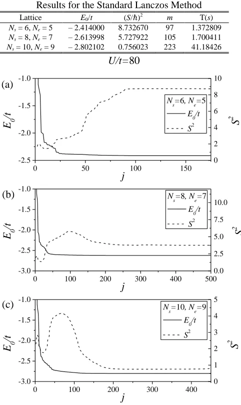
Those results show that for the strong-coupling regime, the standard Lanczos method fails to find a correct ground-state eigenvector. Table II shows the results for the standard Lanczos method using Error > 10-6 as a stopping criterion. It is clear that this parameter is not enough to ensure a robust result for the ground-state vector, since the S2 error remains at the third significant digit, and for the case with Ns = 8, the result is
TABLE II
Results for the Standard Lanczos Method
Lattice E0/t (S/ℏ)2 m T(s) Ns = 6, Ne = 5 – 2.414000 8.732670 97 1.372809
Ns = 8, Ne = 7 – 2.613998 5.727922 105 1.700411
Ns = 10, Ne = 9 – 2.802102 0.756023 223 41.18426
0 50 100 150 -2.5
-2.0 -1.5 -1.0
0 100 200 300 400 500 -3.0
-2.5 -2.0 -1.5 -1.0
0 100 200 300 400 -3.0
-2.5 -2.0 -1.5 -1.0
Ns=6, Ne=5
E
0/t
S2
E
0/t
j
0 2 4 6 8 10
S
2
Ns=8, Ne=7
E0/t
S2
E
0/t
j
0.0 2.5 5.0 7.5 10.0
S
2
N
s=10, Ne=9
E0/t
S2
E
0/t
j
0 1 2 3 4 5
(c)
(b)
S
2
U/t=
80
(a)
Fig. 4. Ground-state energy (solid line) and S2 (dashed line) as a function of j
for a ladder lattice when U/t = 80. j is the number of Lanczos vectors created by the algorithm.
0 50 100 150 200 250
90 100 110 120 130 140
Ns=10, Ne=12
E
0/t
S2
E 0
/
t
j
2 4 6
S
2
Fig. 5. Ground-state energy (solid line) and S2 (dashed line) as a function of j
for a ladder lattice when U/t = 80. j is the number of Lanczos vectors created by the algorithm.
To deal with this, we have created another algorithm that uses S2 as a stopping criterion, which makes it running more iterations until the convergence of the state is achieved, regardless of the energy value. It takes place right after line 10 of Algorithm 1 and has the following form:
Do the Algorithm 2
Diag(a, b, j|E0, V0)
Error = |E0 – E|
S2value(V0|S2) (12)
S2error = S2- Stest
E = E0
Stest = S 2
where S2value(V0|S2) is the calculation of the S2 value using the
ground state vector V0 given by Diag(a, b, j|E0, V0). The
stopping criterion at line 2 must also be modified to
While (Error > X and S2error > Y ). (13)
Due to numerical instabilities in the Lanczos vectors, discused in Sec. II, it was necessary to use X and Y = 10-5, in the stopping criterion, rather than 10-6 (Table III). This approach does not show any improvement in comparison with the cases U/t = 1 and 10. The system with U/t = 80 there was an improvement in the S2 value form a totally incorrect to an error at the third significant digit.
This approach does not show any improvement in comparison with the previous result, and the systems with Ns =
6 and 10 remained with the same accuracy. However the Ns =
8 system shows the same accuracy as the Ns = 6 and 10, which
did not occur before. Thus, for high values of U, the standard Lanczos algorithm produces results with an unacceptable accuracy.
The loss of orthogonality makes the standard Lanczos model a, unreliable method, specially when dealing with quantum state transitions, even using S2 as a stopping criterion.
TABLE III
Results for the Standard Lanczos Method with S2 as stopping criterion
Lattice E0/t (S/ℏ)2 m T(s) Ns = 6, Ne = 5 –2.414202 8.746640 111 1.684811
Ns = 8, Ne = 7 – 2.622987 3.766765 690 142.5225
Ns = 10, Ne = 9 – 2.802102 0.754876 269 397.8961
ERL
processing time it takes to reach the desirable convergence, as shown in Fig. 6 We clearly see that, for higher values of m, the convergence behavior is unstable due to the fact the algorithm generates too many vectors which inducing loss of orthogonality.
These previous evaluations were done using the ERL algorithm, instead of the standard Lanczos procedure. The convergence could be reached when the error between two restarts was less than 10-6 for the energy and less than 10-5 for
S2, as shown in Table IV.
TABLE IV
Results for the ERL-Based Algorithm with S2 as stopping criterion
Lattice E0/t (S/ℏ)2 m T(s) Ns = 6, Ne = 5 –2.414202 8.746640 111 1.684811
Ns = 8, Ne = 7 – 2.622987 3.766765 690 142.5225
Ns = 10, Ne = 9 – 2.802102 0.754876 269 397.8961
The ERL algorithm presented a significant improvement regarding the S2 error rates. Also, the algorithm has a much better processing time, being 5 times faster than the standard method for Ns = 10, and 44 times faster for the unstable case
with Ns = 8. Hence, this methodology turns to be efficient for
intermediate degrees of accuracy.
0 20 40 60 80 100 0
20 40 60 80 100
0 20 40 60 80 100 120 140 160 180 200 0
500 1000 1500 2000 2500
0 20 40 60 80 100 120 140 160 180 200 0
10000 20000 30000 40000 50000
T
(
s
)
m
N
s=
6
, N
e=
5
(a)
T
(
s
)
(b)
T
(
s
)
m
N
s=
8
, N
e=
7
(c)
m
N
s=
10
, N
e=
9
Fig. 6. Processing time as function of the Lanczos matrix dimension, m, of a ladder lattice with U/t = 80.
MERL
The MERL-based algorithm showed better results (see Table V) while the S2 error remained at the last significant digit for all cases. This accuracy improvement comes with a cost in the processing time, which is now approximately two or three times more than in the ERL-based scheme, but still less than the ones found in Table IV. The Better convergence is a result of the decrease in the tridiagonal matrix dimension generated by the method. This decreases the lost of orthogonality discussed in the Lanczos method section.
Due to the changes in the matrix dimension some interaction should be faster than other, which makes a difficult a time analyses. A compared study between ERL and MERL convergence rate was made in [20] using a starting matrix with dimension of three or four and the dimension increase rate of
N + 1. The initial procedure of the algorithm presented in this work is different than the original method proposed by Zhang. We use an starting matrix with dimension of N = 4Ns and we
used a dimension decreased rate of N– 4. These are arbitrary choices based in the fact that the MERL can be easily modified by empirical observations.
TABLE V
Results for the MERL-Based Algorithm with S2 as stopping criterion
Lattice E0/t (S/ℏ)2 m T(s) Ns = 6, Ne = 5 –2.414214 8.750000 111 0.093600
Ns = 8, Ne = 7 – 2.622966 3.750000 690 7.113646
Ns = 10, Ne = 9 – 2.802176 0.750000 269 221.3342
VI. CONCLUSIONS
be used since it yields a better accuracy.
ACKNOWLEDGEMENT
This work was supported by CAPES. We thank G. M. A. Almeida for a careful reading of the manuscript.
REFERENCES
[1] H. E. Stanley, Introduction to Phase Transitions and Critical Phenomena, Oxford Science Publications, 1971.
[2] J. Hubbard, Electron correlations in narrow energy bands, Proceedings of the Royal Society of London A: Mathematical, Physical and Engineering Sciences Vol. 276, Issue 1365, (1963) 238-257.
[3] M. C. Gutzwiller, Effect of correlation on the ferromagnetism of transition metals, Phys. Rev. Lett. 10 (1963) 159-162.
[4] J. Kanamori, Electron correlation and ferromagnetism of transition metals, Progress of Theoretical Physics 30 (3) (1963) 275-289.
[5] M. P. A. Fisher, P.B. Weichman, G. Grinstein, D. S. Fisher, Boson localization and the superfluid-insulator transition, Phys. Rev. B 40 (1989) 546.
[6] M. J. Hartmann, F. G. S. L. Brandao, M. B. Plenio, Laser Photon. Rev. 2 (2008) 527.
[7] M. Vojta, Quantum phase transitions, Reports on Progress in Physics 66 (12) (2003) 2069.
[8] S. Sachdev, Quantum Phase Transitions, Cambridge University Press, 2011.
[9] E. . Lieb, F. Y. Wu, Absence of mott transition in an exact solution of the short-range, one-band model in one dimension, Phys. Rev. Lett. 20 (1968) 1445-1448.
[10] C. Lanczos, An iteration method for the solution of the eigenvalue problem of linear differential and integral operators, J. Res. Nat. Bur. Stand. 45 (1950) 255.
[11] E. Dagotto, Correlated electrons in high-temperature superconductors, Rev. Mod. Phys. 66 (1994) 763-840.
[12] E. R. Gagliano, E. Dagotto, A. Moreo, F. C. Alcaraz, Correlation functions of the antiferromagnetic heisenberg model using a modified lanczos method, Phys. Rev. B 34 (1986) 1677-1682.
[13] C. Broin, L. Nikolopoulos, A {GPGPU} based program to solve the {TDSE} in intense laser fields through the finite difference approach, Computer Physics Communications 185 (6) (2014) 1791-1807. [14] W. Rodrigues, A. Pecchia, M. Lopez, M. A. der Maur, A. D. Carlo,
Accelerating atomistic calculations of quantum energy eigenstates on graphic cards, Computer Physics Communications 185 (10) (2014) 2510-2518.
[15] N. Mohankumar, S. M. Auerbach, On time-step bounds in unitary quantum evolution using the Lanczos method, Computer Physics Communications 175 (7) (2006) 473-481.
[16] T. Siro, A. Harju, Exact diagonalization of the Hubbard model on graphics processing units, Computer Physics Communications 183 (9) (2012) 1884-1889.
[17] A. Ribeiro, C. Macedo, Metallic ferromagnetism in the 3D Hubbard model at finite temperature, Journal of the Korean Physical Society 62 (10) (2013) 1445-1448.
[18] G. H. Golub, C. F. Van Loan, Matrix Computations (3rd Ed.), 3rd Edition, Johns Hopkins University Press, Baltimore, MD, USA, 1996. [19] H.-G. Weikert, H.-D. Meyer, L. S. Cederbaum, F. Tarantelli, Block
Lanczos and many-body theory: Application to the one-particle green's function, The Journal of Chemical Physics 104 (18) (1996) 7122-7138. [20] G. Zhang, Modified explicitly restarted lanczos algorithm, Computer
Physics Communications 109 (1) (1998) 27-33.
[21] P.~Sengupta, A. W. ~Sandvik, D.K. ~Campbell, Bond-order-wave phase and quantum phase transitions in the one-dimensional extended Hubbard model, Phys. Rev. B. 65 (2002) 155113.
[22] T. X. R. Souza and C. A. Macedo. In preparation (2016).