Abstract— Sit to stand (STS) motion has recently been given
an intensive attention by both biomechanical and robotics researchers. STS motion determinants are factors that affect the performance of the STS motion. Determinants differ with their affect based on how they are related to the STS motion, such as chair-related, subject-related and motion-settings-related. Humans who face issues with performing an STS motion find difficulties to perform the motion successfully when they are subjected to wear a prosthetic device. Torque produced by the motors used to help the patients performing a STS motion is one of the parameters that can affect how successful the motion can be performed. Moreover, hip joint’s initial position is one of the parameters that affects the STS motion performed with the aid of the prosthetic devices. It was hypothesized that the relationship between the hip and knee joints initial position and their torque
is not linear. In this project, the objectives were to investigate the effect of changing the hip initial position on the torque required by each joint to successfully perform the STS motion in both experimental and simulation environment. Experiments were conducted to ensure the validity of the hypothesis. The experiments were designed in a way to imitate the human body measurements and the motion was planned in the same way humans do. The torque produced by each joint was fitted and a 2nd degree polynomial relationship was created to predict the maximum and minimum torque based on the hip’ initial position. The results show that the goodness of the line fitting is close to 1, with a confidence level of 95%, ranging from 0.8672 to 0.9799.
I. INTRODUCTION
Human-daily-motion can be categorized into a very wide set of phases and sub phases, like standing, walking and setting. Each of these motions has a different set of sub phases and each of them includes a different set of parameters, characteristics and physical constraints that is different from a person to another. Moreover, the human-muscular actions are different based on the human parameters and environmental parameters which may affect each motion directly. Therefore, a different set of methods and control schemes should be used for each phase of the motion involved in human-daily-motion. Because of these differences, researchers started to investigate a new method that can either change the control method or at least the controller gains which can suit the motion-phase requirements, i.e. hybrid control method [1].
One of the human motions is a sit to stand motion (STS). STS motion can be analyzed as a point to point movement from a statically sitting position to a statically standing position. The analysis of a sit to stand motion has not been
given attention until recently, additionally most of the studies related to a sit to stand motion has only been involving records of the human motion recording before being studied on a robotic system [2], yet most of the studies presented regarding sit to stand motion are concerned with STS stability, balance and energy transfer occurs during a sit to stand motion.
A sit to stand transition is known to be the most mechanically-demanding task that is undertaken during daily activities as well as it is a prerequisite for a gait [3]. According to [4], “the inability to perform a sit to stand transfer can lead to institutionalization, decreased functioning in activities of daily living (ADLs) and in some cases, death”. Optimal coordination, balance, adequate mobility and strength and muscle power output are required for a successful sit to stand to sit motion [5, 6]. Many researchers aim to characterize the sit to stand motion by breaking down it to several stages that identify the start, end and performance of the motion itself [7, 8, 9]. due to the diversity of methods by which the sit to stand motion is characterized, it is a bit challenging to generalize the characteristics of the motion.
In the field of sit to stand motion the main challenge is a part of the motion called chair lift-off, when the support polygon’s area dramatically decreases from the hip touches the chair and the leg touches the base (ground) to be only the leg touching the ground [10]. This very quick and instant (9% of the STS cycle) change causes a very dramatic change in many parameters involved in the STS motion such as the joints torques, velocity and acceleration [11]. A humanoid robot should overcome the changes occur during the STS motion to cease a fall to its back which is called sit-back failure in [10]. According to [12], two main components are involved in the humanoid STS system (1) phase and trajectory planning and (2) motion control. For lift-off issue to be solved a proper combination of proper controller and trajectory planning should be considered during a STS motion [13].
A. Problem Statement
Most of the paralyzed patients who lost their legs due to either an accident, disorder or even a war have been undergoing a vast of issues in their rehabilitation centers as they are physically different. These issues are mainly encountered because of no single setting of a prosthetic leg can be used for all the patients. since every patient differ in terms of mass (m) and length ( ) and their initial position requirements to perform the STS motion successfully. Thus, it is complicated for physicians and engineers in
The Effect of Changing the Hip Joint Initial
Position on the Torque Required to Perform a
Successful Sit to Stand Motion
rehabilitation centers to find a prosthetic leg that can suit all patients.
According to [15], a three-link model is the most suitable model for STS motion analysis as it represents the actual human being body segments. One of the fundamental problems related to the dynamics of any manipulator is when a trajectory point ( ̇ ̈) is given and the required joints torque ( ) is to be found. In the case of STS motion, the torques required by each joint ( ) change in response to any change in the given joints’ initial position ( ) yet the changes that may occur on the torques due to changes in the initial positions is still not obvious.
Since maximum torque produced by the prosthetic leg ( ) may affect its user and leads to unsatisfactory pain and consequences, a simple equation that estimates the maximum torque ( ) changes related to the changes of the patient initial position is a pleasure to these physicians and patients. Some patients are not physically qualified to fulfill the initial position for a minimal joints’ torque requirements; thus, they tend to face difficulties to stand up smoothly. As a result, designing such equation will help to successfully design a prosthetic leg that can suit all patients no matter what their limitations to an initial position are, which will help patients to perform a successful STS motion in their rehabilitation centers.
B. Hypothesis
It is hypothesized that hip and knee initial positions will influence the maximum torque required to perform a successful sit to stand motion. This is because the CoG (center of gravity) will be shifted when there is an angular shift in either hip or knee joint initial position. additionally, the influence on the maximum torque is hypothesized to be non-linear.
C. Research Objectives
The main objectives of this research are to:
1) Investigate the effect of changing the humanoid hip and knee joints’ initial position (θknee_i and θhip_i) on the
maximum torque required (τankle_max, τknee_max and τhip_max) to successfully perform a sit to stand motion.
2) To validate the experimental results by simulating the experimental setup of the STS motion in V-rep Software.
3) To develop a relationship that predicts the maximum torque (τankle_max, τknee_max and τhip_max) required based on the changes of the hip and knee joints’ initial positions (θknee_i and θhip_i).
II. EXPERIMENT
In [1i], STS motion is divided into two distinct phases 1] the forward trunk (CoM transfer phase) and 2] the upward extension (standing phase). However most of the other researchers identify the STS motion into three phases 1] initiation position, 2] seat unloading and 3] lift-off phase [1 itself].
As can be seen in Figure 1, in 1990, Kralj et al [1 j] proposed a Figure that explains and divides the complete
cycle of the sit to stand motion from 0% of the cycle until 100% of the cycle.
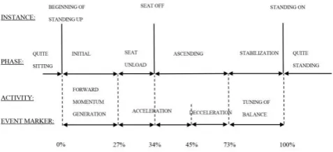
Fig. 1. Sit to stand motion complete cycle.
As can be seen from Figure 1 the first phase of the STS motion is known as quite sitting where it is indicated by the beginning of the motion (0% of the cycle). The forward momentum generation is first part of the beginning of the standing up that is up to 27% of the cycle during which most of the body weight is transferred from the seat to the foot. Right after the forward momentum generation the seat unloading takes place which ends by 34% of the total STS cycle. By 34% of the cycle, where the seat unloading has taken place, the CoM of the body is vertically aligned with the feet to ensure stability during the STS motion. In between 34% and 73% of the cycle the whole body starts to ascend to the standing position which is during 34% to 45% is in acceleration and 45% to 73% is deceleration. The final phase of the cycle which is stabilization of the body is initiated at the 73% of total cycle till it reach to a fully-vertical standing position at the 100% of the STS cycle.
T
ru
n
k
Ɵ1
Ɵ3
Ɵ2
Initial Position (Stationary Setting Position)
Fig. 2. 3 Link Structure.
As can be seen from Figure 2 the robot’s foot is fixed to the ground (base) to avoid the risk of the robot falling down during its operation, moreover the advantage of not fixing the robot does not really affect the research criteria which focuses on changes that may occur if hip and knee initial positions are varied. Leg, tight and trunk are represented by the three links of the humanoid robot shown in Figure 2 link 1, link 2 and link 3 respectively. Additionally, motor 1, motor 2 and motor 3 represent ankle, knee and hip joints respectively.
Figure 3 shows the experiment signals-connection concept.
Motor 3 Motor 1
Motor 2
M
at
lab
S
of
tw
ar
e
Current, A Position, degrees
Current, A Position, degrees
Current, A Position, degrees
Fig. 3. System Overview.
The Matlab software is used to supply the desired position information ( ) to the motors and in return it reads the current values ( , , ) and position values ( ) as well. Using the current values extracted during the STS motion the Matlab software calculates the Torque values ( ) with respect to the given current values using the manufacturer performance graph.
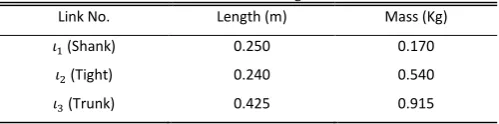
Table 1 shows the lengths and mass measurements of the links used to represent the average human body segments from link 1 to link 3. These measurements are chosen according to De Leva 1996 who represented the actual average human body segments measurements given to each part of the body segment.
TABLE I
Humanoid Robot Mass and Lengths measurement
Link No. Length (m) Mass (Kg)
(Shank) 0.250 0.170
(Tight) 0.240 0.540
(Trunk) 0.425 0.915
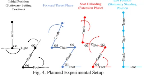
The robot is designed to imitate the human body STS motion which is divided into three phases;
1) Forward thrust phase, during which only the trunk of the robot is moved forward (CW direction) to bring the center of mass of the robot closer to the base which reduces the torque required by the motor before the seat off stage begins. This stage is identified by the start of the hip joint motion to bend the trunk forward.
2) Seat-off phase, during which the loss of contact between the robot and the chair-seat. It is a momentary stage which begins and ends momentarily and can be indicated by the torque value of the hip joint which goes into the opposite direction (CCW) as the motor moves in the other direction of the forward thrust stage.
3) Extension phase, it is the stage where the full extension of the three joints involved in the STS takes place. It involves the movement of the three joints together until a stationary standing up position is fulfilled.
A. Experimental Objectives
The main objectives of these experiments are 1) to design a setup that experimentally performs a STS motion to investigate the maximum torque,
( ) changes that occur due to changing the initial position of both joints, knee and hip. 2) to validate the experimental results by simulating the STS motion in V-rep software to investigate the changes that may occur when hip and knee initial positions change. The experimental torque changes are fitted using curve fitting toolbox in Matlab. Using the data from curve fitting relationship that can easily predict each joint’s maximum torque required to perform a successful STS motion if body initial positions are altered and known.
B. Experimental Equipment and Parameters
Follows is the list of the experimental equipment used to conduct the experiment:
1) 3 Dynamixel MX-106 motors.
2) USB2Dynamixel adapter.
3) 12V, 5A AC adapter.
4) SMPS2Dynamixel power supply adapter to Dynamixel bus.
5) Matlab Software.
C. Experimental Setup
perform a successful STS motion several data needs to be collected and analyzed during the experiment. The robot undergoes the three phases of STS motion and during each phase data is collected and analyzed thoroughly. Using the built-in current sensor in the motor itself the instant current value is read and saved during the time taken of the STS to be performed. Moreover, the position value using the built-in encoder is read and saved as well. From the manufacturer performance graph, the torque value is extracted using the respective current value for a further analysis.
Figure 4 show the phases through which the robot goes through for a complete sit to stand motion cycle.
T
ru
n
k
Ɵ1 Ɵ3 Ɵ2 Initial Position (Stationary Setting
Position)
Foot Ɵ1 Ɵ3 Ɵ2
Forward Thrust Phase
Foot Ɵ1 Ɵ3 Ɵ2
Seat-Unloading (Extension Phase)
Foot
Sh
an
k
T
ig
h
t
T
ru
n
k
End Position (Stationary Standing
Position
Fig. 4. Planned Experimental Setup
Figure 4 shows one of the experimental setups used in this research. As can be seen in Figure 4 the robot is initially in a sitting position with the initial states of θ1 = 670, θ2 =1130 and θ3 =2700. During the first phase (forward-thrust phase) the power is supplied to the motors and only link 3 (trunk) is involved in this phase as it moves in clockwise direction from 2700 to 2250 with respect to link 2 (tight). The second phase is initiated by the start of the seat-off where the supporting polygon shifts from the chair’s seat and foot to be only the foot, where the knee joint moves in clockwise direction (1130-00) and this momentarily initiates the third phase which is the extension-phase, where both the hip (2250-3600) and ankle (670-900) joints move in counterclockwise direction and the knee joint moves in clockwise direction, that ends by a stationary fully extended joints’ positions as illustrated in Figure 4.
The experimental setup shown in Figure 4 is repeated with change the hip initial position from 2700 to 2150 and change of knee initial position from 780 to 1330 with every single change of the hip initial position.
Table 2 shows initial positions and desired positions for the three joints (ankle, knee and hip) during the initial phase, Phase 1 and Phase 2.
TABLE II
Experiment States Joints’ Positions.
Phase
Initial Phase
67
078
0270
0Phase1
67
078
0270
0Phase2
90
00
0360
0The experiments are repeated for every 50 increments from 780 to 1330 of the knee initial position during the initial phase. Additionally, the experiments are repeated for every 50 decrements from 2700 to 2150 of the hip initial position during Phase1.
As can be seen from Table 2, only hip joint is involved during phase 1 where it moves in CW direction from 270o to
215o for experiments 1-12, respectively. Both ankle and knee joints remain stationary during phase 1 of the STS motion. During phase 2 the hip and ankle joints start moving to 3600 and 900 in a CCW direction respectively. While the knee joint moves in CW direction from 1130 to 00 at which the body reaches a fully-extended state and this where the STS motion reaches 100% of its cycle.
D. Procedure
Table 3 shows the Dynamixel MX-106 specifications given by the manufacturer in its user manual.
TABLE III
Dynamixel MX-106 Servo Motor Specification
Model MX-106T
Stall Torque @ 12V 8.4N.m
Speed (rpm) @ 12V 45
Operating Voltage 10V~ 14.8V (Recommended
Voltage 12V)
Stall Current Draw 6.3A
Dimensions 40.2mm*65.1mm*46mm
Weight 153g
Resolution 0.088o
Operating Angle 360
Gear Reduction 225:1
Gear-Train Material Hardened Steel
Position Sensor Magnetic Encoder
Figure 5 shows the USB2Dynamixel application concept which connects Dynamixel motors in series and interfaces the motors with the PC through a USB bus.
Fig. 5. USB2Dynamixel Application Concept
Start
Initial Position of the Humanoid Robot Joints
Matlab Signals Desired Positions to Hip Joint Only.
Trunk Bends Forward Till it Reaches Desired Position
Matlab Signals Desired Position to Ankle, knee and
hip joints.
Joints Move to Desired Positions
Joints Torque Values are extracted from the current
values for each joint
END
Phase 1
Phase 2 Joints position
and current values are recorded.
Joints position and current
values are recorded.
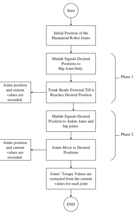
Fig. 6. Flow of the Processes during the Experiment Conduction
Figure 6 show the processes of the above explained phases. Where the system starts where the robot is placed on a chair with the initial position settings, then the Matlab software signals the desired position information to the hip joint. Hip joint responses to the data given and starts bending forward to the desired position during Phase1, meanwhile the position and current data is recorded. Then the desired position is sent to the ankle, knee and hip joints and they move correspondingly where the position and current data are recorded as well for further analysis, where the torque values are extracted from the current data collected.
E. Precautions on Validity Issues
Measurements of the humanoid robot follows the average human mass and length measurements which is taken from Paolo De Leva (1996) in his journal of biomechanics studies. Yet the humanoid robot links’ lengths used is reduced by 1.7 of the actual human average length, while the robot mass follows the percentage distribution of average human mass proposed in Paolo De Leva (1996).
The trajectory of the humanoid robot is generated using the cubic polynomial technique. Each joint’s trajectory is generated separately based on both the initial and desired joint positions. The cubic polynomial Equation generates the positions through which each joint has to go through to reach its desired position, and this explains the existence of some vibrations on the motors motion, since every single position
information has to be followed by the motor before it reaches its desired (final) position.
Position and current values are extracted using the built-in encoder and current sensor respectively. Using Equation 1 in Section F the angular position of the motor is found, while using Equation 2 in Section F the current value is found. Both Equations are provided by the manufacturer of the motor which could be found in the motor’s user manual. Torque is generated using the found current value and the Equation 3 that is generated from the performance graph given by the Robotis co.
The time taken for the STS motion has been set to 6 seconds based on the experimental work conducted during this research. As it has shown that the user could obtain as much data as possible to be analyzed and further discussed, while bearing in mind a logical time consumption for a STS motion to be successfully performed.
Last but not least, the foot of the robot is fixed to the base since not fixing it will not result in any changes in the data read during the experiment conduction, especially for the criteria studied in this research.
F. Methods of Analysis
With reference to the manufacturer manual of the Dynamixel MX-106T, the following is a list of the parameters involved in the experiment and their related Equations:
Goal position (θd) motor range value is from 0-4095 and the unit for each is 0.0880, hence the motor angular position can be obtained using equation 1.
θd = Motor Value × 0.0880 (1)
Actual Position (θa) range value is from 0-4095 as well and the same Equation is used to obtain actual position with ±2° error as indicated by the manufacturer manual.
The actual current value that is drawn by the motor coil is of a value 2048 when current is consumption is idle meaning that 100mA is consumed by the motor circuitry. Values are higher than 2048 during positive current flow and lower than 2048 during negative current flow. The following method is to calculate current flow to the motor coil;
I = (4.5mA) × (Motor Value-2048) in amp unit(A) (2)
Based on the current vs torque performance graph, the torque is calculated as follow:
τ = (-0.1596495 × I2) + (2.007124 ×I) (3)
III. RESULTS AND DISCUSSION
A. Joints Position during STS Motion
Fig. 7. Theoretical vs Experimental Joints’ Position during phase 1
Fig. 8. Theoretical vs Experimental Joints Position during phase 2
As can be seen from Figure 7, during phase 1 the hip joint is the only joint involved in the STS motion where it moves from 2700 degrees to 2250 degrees in CW direction. Meanwhile both the knee and ankle joints are stationary at 1130 degrees and 670 degrees respectively.
During phase 2 which is shown in Figure 8, the hip joint starts to move in the CCW direction and the seat-off phase is initiated, the hip moves in the opposite direction from 225 degrees to 360 degrees with respect to link 2. While the knee joint starts lifting up the tight and trunk of the robot from 90 degrees to 0 degree in CW direction and the ankle joint moves in the CCW direction from 67 degrees to 90 degrees with respect to the stationary base.
It can be clearly seen that the time taken for phase 1 is 2 seconds and phase 2 is 4 seconds which makes the total time taken for a successful STS motion is 6 seconds. It is considered as a long time for a STS to be performed by a healthy human, but for the purpose of data collection and speed of the data reading between Matlab and the Dynamixel MX106 6 seconds is found to be the most suitable time based on the experimental trials conducted.
Moreover, from Figures 7 and 8 it can be clearly seen that there are some fluctuations in the actual position values
which are due to the position-control method used to move the motors as the motor struggle to follow every single position data generated by the cubic polynomial. Thus, vibrations can be clearly seen in the graphs despite the fact that all of the motor managed to reach the final position within the generated trajectory (actual position).
B. Joints Torque During STS Motion
Figures 9 and 10 show the actual torque graphs of the joints during STS motion in both phase 1 and 2 respectively with a 2250 and 1130 of angular position for hip and knee joints respectively.
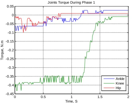
Fig. 9. Actual Joints Torque during Phase 1
Figure 9 shows the actual measured torque of the three joints during phase 1. It is obvious that torque at the knee is the highest due to the body weight is mostly loaded on the knee joint. Yet all of the joints have some values of torques due to the motors struggling to stay stationary which means that there is an amount of current flowing into the motor coil, despite the fact that the motors are not moving during phase 1. For hip and ankle joint torques the maximum value reached is -0.1 N.m and -0.09 N.m, respectively. Hip and ankle joints are struggling from falling down under the effect of the gravity, thus they are acting in a CCW direction to hold the joint stationary. On the other hand, knee maximum torque value is approximately -0.43 N.m. Since it is struggling to hold the knee joint in a CW direction to hold it stationary in its place since it is not moving during phase 1. 0 0.2 0.4 0.6 0.8 1 1.2 1.4 1.6 1.8 2
50 100 150 200 250 300
Theoritical vs Actual Joints Position During Phase 1
Time, S
P
o
s
it
io
n
,
D
e
g
re
e
Actual Ankle Actual Knee Actual Hip Theoritical Ankle Theoritical Knee Theoritical Hip
2 2.5 3 3.5 4 4.5 5 5.5 6
0 50 100 150 200 250 300 350 400
Theoritical vs Actual Joints Position During Phase 2
Time, S
P
o
s
it
io
n
,
De
g
re
e
Actual Ankle Actual Knee Actual Hip Theoritical Ankle Theoritical Knee Theoritical Hip
0 0.5 1 1.5 2
-0.45 -0.4 -0.35 -0.3 -0.25 -0.2 -0.15 -0.1 -0.05 0 0.05
Joints Torque During Phase 1
Time, S
T
o
rq
u
e
,
N.
m
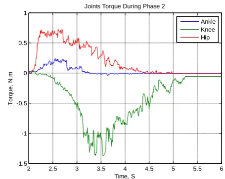
Fig. 10. Actual Joints Torque during Phase 2
Figure 10 shows the actual torque values of the joints performing the STS motion during phase 2. Ankle and hip joints torques are of positive values as both of the joints are moving in the CCW direction. On the other hand, the knee joint is in the negative direction as the joint is moving in the CW direction. Ankle joint is exerting the lowest torque value of 0.2415 N.m as it is moving from 67 degrees to 90 degrees with minimal body weight being loaded onto the joint. While in contrast the hip joint is exerting a torque value of 0.7274 N.m which is higher than the ankle joint by 0.4859 N.m as the mass being loaded on the joint alone is about 0.915 Kg. Knee joint is exerting the highest torque value of a -1.3776 N.m as most of the body mass is being loaded on the knee joint. As it can be seen from Figure 10, the torque values end with a value of 0 N.m for all of the joints as they reach to a fully extended position (standing-position).
Figures 11 and 12 show the simulation and experimental 3D surface graphs of the ankle-joint maximum torque values versus the knee and hip initial positions respectively.
Fig. 11. Simulation Results of the Maximum Ankle Torque vs. Hip and Knee Initial Positions
Fig. 12. Experimental Results of the Maximum Ankle Torque vs. Hip and Knee Initial Positions
As can be seen from Figure 11 the maximum ankle torque increases in the direction of increasing the hip initial position. on the other hand, the ankle maximum torque seems to be at its maximum values during the 1130 of the knee initial position and it decreases in a symmetric way around the 1130 as can be seen in Figure 11. The ankle torque varies from approximately 0.19 N.m to 0.7 N.m. As can be observed from Figure 11 the minimum torque appears to be at the 2130 and 780 of the hip and knee initial positions respectively. Concurrently, the maximum torque appears to be at the 2700 and 1130 of the hip and knee initial positions respectively.
In Figure 12 the surface, representing the maximum ankle torque, increases in the direction of decreasing the knee initial position from 1400 to 700. Concurrently, the maximum ankle torque increases in the direction of decreasing the hip initial position from 2700 to 2150. It can be seen from Figure 12 that the ankle torque varies from the minimum torque value of -0.3665 N.m to a maximum value of 1.0455 N.m to successfully perform an STS motion. The experimental settings for minimum torque appears to be at 2700 of hip angle and 1280 of knee angle. Alternatively, the maximum torque value appears to be at 2300 of hip angle and 830 of knee angle. The surface graph in Figure 12 shows some fluctuation in the peak values of the ankle torque due to expected random errors of the motor current feedback.
Figures 13 and 14 show the simulation and experimental 3D surface graphs of the knee-joint maximum torque values versus the knee and hip initial positions respectively.
2 2.5 3 3.5 4 4.5 5 5.5 6
-1.5 -1 -0.5 0 0.5 1
Joints Torque During Phase 2
Time, S
T
o
rq
u
e
,
N.
m
Fig. 13. Simulation Results of the Maximum Knee Torque vs. Hip and Knee Initial Positions
Fig. 14. Experimental Results of the Maximum Knee Torque vs. Hip and Knee Initial Positions
The simulation results of the maximum knee torque vs. the hip and knee initial positions is shown in Figure 13. As can be seen from Figure 13 the maximum knee torque increases in the direction of decreasing the knee initial position. It can be clearly seen that the knee maximum torque seems to be at its maximum values during the 1330 of the knee initial position and it decreases in gradually until it reaches 780 as can be seen in Figure 13. The knee torque varies from approximately 4.15 N.m to 1.0 N.m. As can be observed from Figure 13 the minimum torque appears to be at the 780 of the knee initial positions. Moreover, the negative toque values indicate that the torque direction is in the CW direction.
As can be seen in Figure 14, the surface graph, representing the knee maximum torque, increases with the increase of the knee initial position from 700 to 1400. Moreover, the torque increases with the increase of the hip initial position from 2150 to 2700. The knee maximum torque varies from -0.4223 N.m as the minimum value to -3.0116 as the maximum value. The maximum torque value is found to be at the experimental settings of 2650 of the hip position and 1280 of knee position., while the minimum torque value is found to be at 2250 of the hip initial position and 780 of the knee initial position. the negative value of the torque indicates the CW direction of the maximum knee torque to successfully perform the STS motion.
Figures 15 and 16 show the simulation and experimental 3D surface graphs of the hip-joint maximum torque values versus the knee and hip initial positions respectively.
Fig. 15. Simulation Results of the Maximum Hip Torque vs. Hip and Knee Initial Positions
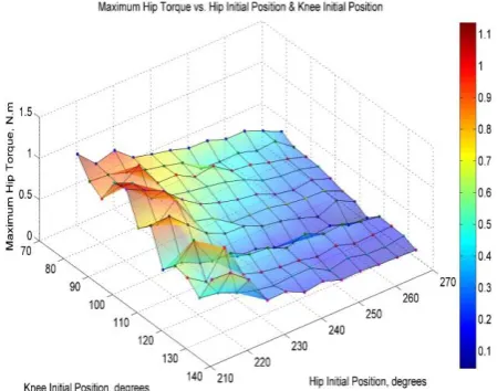
Fig. 16. Experimental Results of the Maximum Hip Torque vs. Hip and Knee Initial Positions
Figure 15 shows the simulations results of the maximum hip torque surface graph of different experimental settings for both hip and knee initial positions. As it can be seen from the graph, the maximum hip torque increases with the decrease of the angular position of both the hip and knee joint from 2700 to 2150 and 1400 to 700 respectively. The maximum hip joint torque varies from 0.361 N.m to 1.19 N.m. The maximum torque is found to be at the experimental settings of 2150 and 830, while the minimum torque is found to be at the 2700 and 1330 of the hip and knee joints respectively. The torque values are positive since the hip joint is moving in the CCW direction.
joints respectively. The torque values are positive due to the CCW direction of the hip joint to perform a successful STS motion. Some fluctuations appear on the surface graph of the maximum hip joint torque due to expected random errors of the motor current feedback.
C. Curve Fitting of the Maximum Joints Torque
Below are the curve fitting results of the trunk initial position being changed from 2700 to 2150 and the knee initial position changed from 1330 to 780 vs. the maximum torque of the three joints involved in the STS motion during phase 2.
Figures 17 and 18 show the curve fitting of the maximum and minimum ankle torque vs. the trunk initial position using 2nd degree polynomial fitting, respectively.
1) Ankle Joint
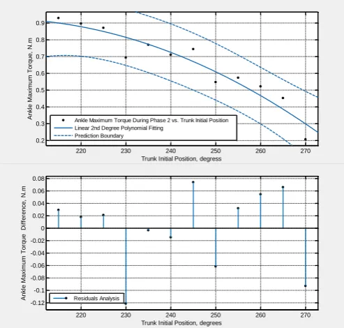
Figures 17 and 18 show the curve fitting of the maximum and minimum ankle torque vs. the trunk initial position using 2nd degree polynomial fitting, respectively.
Maximum Produced-Torque Equation:
(4)
Equation 4 shows how the maximum ankle torque is calculated when the trunk initial position is known ( ). The coefficients are generated with a 95% confidence bound where ranges from -0.0003018 to 0.00003989, ranges from -0.03032 to 0.1335 and ranges from -14.37 to 5.664. The goodness of the curve fitting done by the curve-fitting toolbox in Matlab is shown to be 0.9116.
Fig. 17. Curve Fitting of the Ankle Maximum Torque vs. the Trunk Initial Position Using 2nd degree Polynomial Fitting.
Minimum Produced-Torque Equation
(5)
Equation 5 shows how the minimum ankle torque is calculated when the trunk initial position is known ( ). The coefficients are generated with a 95% confidence bound where ranges from -0.00004346 to 0.0001023, ranges from -0.05338 to 0.01736 and ranges from -1.894 to 6.653. The goodness of the curve fitting done by the curve-fitting toolbox in Matlab is shown to be 0.8672.
Fig 18. Curve Fitting of the Minimum Ankle Torque vs. the Trunk Initial Position Using 2nd degree Polynomial Fitting.
In Figures 17 and 18 the 2nd degree polynomial is used to fit the data collected for the maximum and minimum ankle torque required to successfully perform a STS motion versus the trunk initial position, respectively. The two boundaries around the fitted line in Figures 17 and 18 are shown, where the new torque observations of different initial trunk positions are predicted to be within the boundaries shown with a certainty level of 95%. The lower graph of Figures 17 and 18 shows the residual analysis which presents the difference between the response data (actual data) and the fit to the response data (theoretical data), which mathematically predicts the random errors for maximum and minimum ankle torque values respectively. It is shown that the residuals behave randomly around the zero line which suggests that the model fits the data well with a maximum approximated error of 0.12 N.m for maximum ankle torque and 0.055 N.m for the minimum ankle torque.
2) Knee Joint
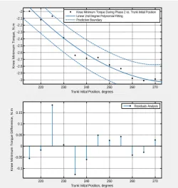
Figures 19 and 20 show the curve fitting of the maximum and minimum knee torque vs. the trunk initial position using 2nd degree polynomial fitting, respectively.
220 230 240 250 260 270 0.2 0.3 0.4 0.5 0.6 0.7 0.8 0.9
Trunk Initial Position, degress
A n k le M a x im u m T o rq u e , N. m
Ankle Maximum Torque During Phase 2 vs. Trunk Initial Position Linear 2nd Degree Polynomial Fitting
Prediction Boundary
220 230 240 250 260 270 -0.12 -0.1 -0.08 -0.06 -0.04 -0.02 0 0.02 0.04 0.06 0.08
Trunk Initial Position, degrees
A n k le M a x im u m T o rq u e Di ff e re n c e , N. m Residuals Analysis
220 230 240 250 260 270
-0.35 -0.3 -0.25 -0.2 -0.15
Trunk Initial Position, degrees
A n k le M in im u m T o rq u e , N. m
Ankle Minimum Torque During Phase 2 vs. Trunk Initial Position Linear 2nd Degree Polynomial Fitting
Prediction Boundary
220 230 240 250 260 270
-0.05 -0.04 -0.03 -0.02 -0.01 0 0.01 0.02 0.03
Trunk Initial Position
Maximum Produced-Torque Equation
(6)
Equation 6 shows how the maximum knee torque is calculated when the trunk initial position is known ( ). The coefficients are generated with a 95% confidence bound where ranges from -0.0001002 to 0.000237, ranges from -0.1278 to 0.03587 and ranges from -3.579 to 16.19. The goodness of the curve fitting done by the curve-fitting toolbox in Matlab is shown to be 0.9337.
Fig. 19. Curve Fitting of the Maximum Knee Torque vs. the Trunk Initial Position Using 2nd degree Polynomial Fitting.
Minimum Produced-Torque Equation
(7)
Equation 7 shows how the minimum knee torque is calculated when the trunk initial position is known ( ). The coefficients are generated with a 95% confidence bound where ranges from 0.00004883 to 0.0004699, ranges from -0.2475 to -0.04316 and ranges from 4.971 to 29.65. The goodness of the curve fitting done by the curve-fitting toolbox in Matlab is shown to be 0.9562.
Fig. 20. Curve Fitting of the Minimum Knee Torque vs. the Trunk Initial Position Using 2nd degree Polynomial Fitting.
In Figures 19 and 20 the 2nd degree polynomial is used to fit the data collected for the maximum and minimum knee torque required to successfully perform a STS motion versus the trunk initial position, respectively. The two boundaries around the fitted line in Figures 19 and 20 are shown, where the new torque observations of different initial trunk positions are predicted to be within the boundaries shown with a certainty level of 95%. The lower graph of Figures 19 and 20 shows the residual analysis which presents the difference between the response data (actual data) and the fit to the response data (theoretical data), which mathematically predicts the random errors for maximum and minimum knee torque values respectively. It is shown that the residuals behave randomly around the zero line which suggests that the model fits the data well with a maximum approximated error of 0.15 N.m for maximum knee torque and 0.175 N.m for the minimum knee torque.
3) Hip Joint
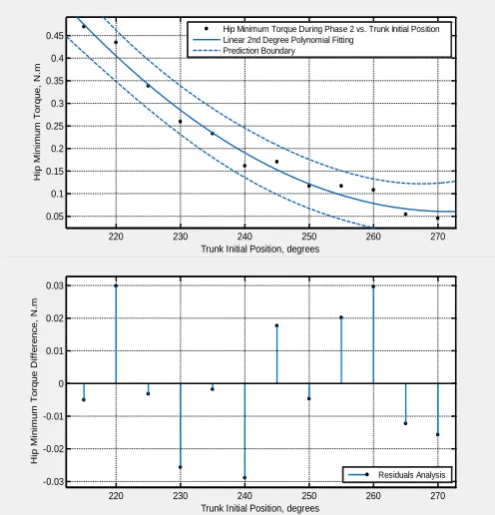
Figures 21 and 22 show the curve fitting of the maximum and minimum hip torque vs. the trunk initial position using 2nd degree polynomial fitting, respectively.
Maximum Produced-Torque Equation
(8)
Equation 8 shows how the maximum hip torque is calculated when the trunk initial position is known ( ). The coefficients are generated with a 95% confidence bound where ranges from 0.000001284 to 0.0002326, ranges from -0.1264 to -0.01414 and ranges from 4.049 to 17.61. The goodness of the curve fitting done by the curve-fitting toolbox in Matlab is shown to be 0.9714.
220 230 240 250 260 270 -1.1 -1 -0.9 -0.8 -0.7 -0.6 -0.5 -0.4
Trunk Initial Position, degrees
K n e e M a x im u m T o rq u e , N. m
Knee Maximum Torque During Phase 2 vs. Trunk Initial Position Linear 2nd Degree Polynomial Fitting
Prediction Boundary
220 230 240 250 260 270 -0.06 -0.04 -0.02 0 0.02 0.04 0.06 0.08 0.1 0.12 0.14
Trunk Initial Position, degrees
K n e e M a x im u m T o rq u e Di ff e re n c e , N. m Residuals Analysis
220 230 240 250 260 270
-3 -2.9 -2.8 -2.7 -2.6 -2.5 -2.4 -2.3 -2.2 -2.1 -2
Trunk Initial Position, degrees
K n e e M in im u m T o rq u e , N. m
Knee Minimum Torque During Phase 2 vs. Trunk Initial Position Linear 2nd Degree Polynomial Fitting
Prediction Boundary
220 230 240 250 260 270
-0.1 -0.05 0 0.05 0.1 0.15
Trunk Initial Position, degrees
Fig. 21. Curve Fitting of the Maximum Hip Torque vs. the Trunk Initial Position Using 2nd degree Polynomial Fitting.
Minimum Produced-Torque Equation
(9)
Equation 9 shows how the minimum hip torque is calculated when the trunk initial position is known ( ). The coefficients are generated with a 95% confidence bound where ranges from 0.0000732 to 0.0001831, ranges from -0.09635 to -0.04301 and ranges from 6.31 to 12.75. The goodness of the curve fitting done by the curve-fitting toolbox in Matlab is shown to be 0.9799.
Fig. 22. Curve Fitting of the Minimum Hip Torque vs. the Trunk Initial Position Using 2nd degree Polynomial Fitting.
In Figures 21 and 22 the 2nd degree polynomial is used to fit the data collected for the maximum and minimum hip torque required to successfully perform a STS motion versus the trunk initial position, respectively. The two boundaries around the fitted line in Figures 21 and 22 are shown, where the new torque observations of different initial trunk positions are predicted to be within the boundaries shown with a certainty level of 95%. The lower graph of Figures 21 and 22 shows the residual analysis which presents the difference between the response data (actual data) and the fit to the response data (theoretical data), which mathematically predicts the random errors for maximum and minimum hip torque values respectively. It is shown that the residuals behave randomly around the zero line which suggests that the model fits the data well with a maximum approximated error of 0.07 N.m for maximum hip torque and 0.03 N.m for the minimum hip torque.
IV. CONCLUSION
This paper has presented an analysis of sit to stand (STS) motion performed by a humanoid robot. The humanoid robot has been designed in a way to represent the human body segments by using Dynamixel (MX-T106) motors to represent the body joints. Furthermore, the STS motion has been designed in a way to simulate the actual human STS motion. The motion has been evaluated by measuring the position and the current values collected during the performance of the STS motion, which were used to obtain the torque values using the motors’ current-torque curve provided by the manufacturer. During the performance of STS motion, hip and knee initial positions have been changed repeatedly to investigate the effect of simultaneously changing the hip and knee initial positions on the torque required to successfully perform STS motion.
The relationship between hip and knee initial positions and the torque, required to perform a successful STS motion, has been hypothesized to be non-linear. The system has shown a 2nd order polynomial relationship after processing the data collected during the performance of the STS motion while changing the initial position settings. Matlab software has been used to process the data and generate the equations relating the torque values with the hip and knee initial position.
The advancement of this research is that it has presented a study that focuses on the changes may occur to a patient performing a sit to stand motion if he/she changes his/her initial position, rather than other parameters that have been studied previously.
V. ACKNOWLEDGEMENT
Authors would like to greatly express their thanks and appreciation to UTeM Center for Research and Innovation Management (CRIM) for their encouragement, help and financial support. This project was conducted in Center of Excellence in Robotics and Industrial Automation (CERIA) in University Technical Malaysia Melaka (UTeM).
REFERENCES
[1] S. Oh, E. Baek, S. K. Song, S. Mohammed, D. Jeon, and K. Kong, “A generalized control framework of assistive controllers
220 230 240 250 260 270
0.3 0.4 0.5 0.6 0.7 0.8 0.9 1 1.1
Trunk Initial Position, degrees
Hi p M a x im u m T o rq u e , N. m
Hip Maximum Torque During Phase 2 vs. Trunk Initial Position Linear 2nd Degree Polynomial Fitting
Prediction Boundary
220 230 240 250 260 270
-0.06 -0.04 -0.02 0 0.02 0.04 0.06
Trunk Initial Position, degrees
Hi p M a x im u m T o rq u e Di ff e re n c e , N. m Residuals Analysis
220 230 240 250 260 270
0.05 0.1 0.15 0.2 0.25 0.3 0.35 0.4 0.45
Trunk Initial Position, degrees
Hi p M in im u m T o rq u e , N. m
Hip Minimum Torque During Phase 2 vs. Trunk Initial Position Linear 2nd Degree Polynomial Fitting
Prediction Boundary
220 230 240 250 260 270
-0.03 -0.02 -0.01 0 0.01 0.02 0.03
Trunk Initial Position, degrees
and its application to lower limb exoskeletons,” Rob. Auton. Syst., vol. 73, pp. 68–77, 2015.
[2] M. Mistry, A. Murai, K. Yamane, and J. Hodgins, “Sit-to-Stand Task on a Humanoid Robot from Human Demonstration,” no. 2, pp. 218–223, 2010.
[3] W. G. M. Janssen, H. B. J. Bussmann and H. J. Stam, “Determinants of the sit-to-sstand movement: a review,” J. Am.
Physical Therapy Assoc., vol. 82, no. 9, pp. 866-879, Sept. 2002.
[4] I. Veledar, A. Arcelus, R. Goubran, F. Knoefel, H. Sveistrup and M. Bilodeau, “Sit to stand timing measurements using pressure sensitive technology,” Proc. IEEE Instrum. Meas. Tech. (I2MTC), pp. 1337-1340, May 2010.
[5] E. L. Cadore and M. Izquierdo, “New strategies for the concurrent strength-, power-, and endurance-training prescription in elderly individuals,”J. Am. Med. Dir. Assoc., vol. 14, no. 8, pp. 623–624, Aug. 2013.
[6] P. O. Riley, D. E. Krebs, and R. A. Popat, “Biomechanical analysis of failed sit-to-stand,” IEEE Trans. Rehabil. Eng., vol. 4, pp. 353–359, Dec. 1997.
[7] A. Arcelus, I. Veledar, R. Goubran, F. Knoefel, M. Bilodeau, and H. Sveistrup, "Measurements of sit-to-stand timing and symmetry from bed pressure sensors," IEEE Trans. Instrum. Meas., vol. 60, no. 5, pp. 1732 1740, May 2011.
[8] T. Banerjee, M. Skubic, J. M. Keller and C. Abbott, “Sit-to-stand measurement for in home monitoring using voxel analysis,” IEEE J Biomed Health Inform., Epub Oct. 2013.
[9] H. Shen, Q. Song, X. Deng, Y. Zhao Y. Yu and Y. Ge, “Recognition of phases in sit-to-stand motion by neural network ensemble (NNE) for power assist robot,” Proc. IEEE Robotics and Biomimetrics, pp. 1703-1708, Dec. 2007.
[10] B. Bahar, M. F. Miskon, N. A. Bakar, A. Z. Shukor, and F. Ali, “Australian Journal of Basic and Applied Sciences,” vol. 8, no. February, pp. 168–182, 2014.
[11] M. B. Bahar, M. F. Miskon, N. A. Bakar, F. Ali, and A. Z. Shukor, “STS Motion Control Using Humanoid Robot,” vol. 8, no. 1, pp. 95–108, 2014.
[12] P. Macdonald, The Alexander Technique: As I See It: Sussex Academic Press, 1989.
[13] P. O. Riley, et aI., "Momentum analysis of sitback failures in sit-to-stand trials," in IEEE 17th Annual Conference on Engineering in Medicine and Biology Society, 1995, vol.2 pp. 1283-1284. [14] M. Z. Ghazali, U. Teknikal, and H. T. Jaya, “A NALYSIS OF T
HREE -LINK POSITION CONTROL DURING SIT TO STAND MOTION,” pp. 1–7.
[15] Ghazali, M.Z., Miskon, M.F., Ali, F. and Bahar, D.M.B., 2016. Analysis of Three-Link Position Control during Sit to Stand Motion. Journal of Telecommunication, Electronic and Computer Engineering (JTEC), 8(7), pp.77-82.
[16] bin Ghazali, M.Z., Miskon, M.F., bin Ali, F. and bin Bahar, M.B., 2015, October. Investigating the relationship between TIP and 3-link models when the links' length are varied. In Robotics and Intelligent Sensors (IRIS), 2015 IEEE International Symposium on (pp. 202-207). IEEE.