174005-1706-3838-IJMME-IJENS © October 2017 IJENS I J E N S
Optimization Design of Open Circuit Wind
Tunnel Suction Type
Ismail
*, Johanis John, Wina Libyawati, Damora Rhakasywi, Agri Suwandi,
Priska Alfatri
Hendrayanto
Department of Mechanical Engineering, Faculty of Engineering, Universitas Pancasila, Jl. Srengseng Sawah, Jagakarsa, Jakarta Selatan 12640, Indonesia
Corresponding author ([email protected])
Abstract— This study present optimize design of open circuit wind tunnel suction type based on the cross section shape variation, whist the specification of the axial fan is set at the debit of 8.75 m3/s and the diameter of 1.250 m. TEA (Task Episode Accumulation) and Computational Fluid Dynamic (with Ansys 15.0 version) applied in this study to determine the optimum design. The outcome is wind tunnel design variation 6 has the highest performance among others design. Variation 6 has a length of 5.015 m, speed of 15.0 m/s, Reynolds number of 8.1 x 10⁵, turbulence intensity ranging between 10.25-10.75%, and the specimen must be placed in the middle of plane III and plane III in order to form uniformity in flow.
Index Term— Computational Fluid Dynamic, Design, Open Circuit, Wind Tunnel
I. INTRODUCTION
Aerodynamic research is un-separable from a test tool called wind tunnel. Wind tunnel is a tool to analyze the influence of winds movement which surrounded solid objects. The principles of wind tunnel is applied wind-blowing system in a venture tube room, which consist of test section and test compartment, also equipped with a measuring instrument. Previous studies related to wind tunnel mainly discussed about: the experimental testing of turbine blade performance due to variation of loads [1]; measurement of the wind flow distribution [2]; correlation model between variation of wind velocity and transition process phenomena at the boundary layer [3]; comparison between experimental and simulation testing by putting resistance in certain zone in order to obtain pressure gradient [4]–[18]. The result of those studies shown, that fluid mechanics theory plays an important role to understand aerodynamic problems.
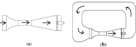
Fluid mechanic non dimensional parameter which influence the performance of wind tunnel are: Reynolds, Mach, Prandlt, Euler, Eckert, Froude and Strouhal number [19]; the boundary level number and layer number [20]. Types of wind turbine are open and closed channel. Figure 1 resumes the different shape between open and closed channel. The different among it requires measurement instrument in order to obtain turbulence level, fluid mechanics parameter. Closed circuit tunnel performance depends on the hypersonic speed achievement, while open circuit depends on subsonic speed.
Fig. 1.. Open circuit wind tunnel scheme (a), Closed circuit wind tunnel (b)
Wind tunnel design is escalating with the aids from design software, which has an ability to make CAD model and to implement finite element method to analyze the flow pattern inside the wind tunnel. Aside that the implementation of the software design useful to design dimension and shape of the contraction chamber [21]–[24], to make pressure changes simulation together with the simulation of flow within the wind tunnel [25]. The simulation result become a recommendation for the designer to modify crucial parameters in order reduces the turbulence intensity in the wind tunnel [26]. Turbulence kinetic energy and flow velocity are the common parameter to determine the performance of wind tunnel. Both parameters can be obtained from Computer Fluid Dynamic (CFD) simulation and experimental result. CFD simulation and experimental result complement each other.
Certain advantages are required in CFD methods such as its ability to complete nonlinear fluid flow physics, although it has to linearly impact on computer resources [27]. But the problem of computer resources in the optimization can is interrogated by using Ullman method or other methods such as Surrogate-Based Optimization (SBO) method. For example the use of the CFD method is to solve the problem of flow through wind turbines, and simulation of flow through wind turbines with some models of CFD turbulence can be relied upon as aerodynamic wind turbine properties [28]. The design of the wind turbine blades must meet the aerodynamic criteria and with the turbulence model on the CFD can be done an analysis. Another advantage is to know the performance of a wind tunnel or one part of a wind tunnel such as a diffuser [29]. The diffuser is located after the test chamber serves to reduce the flow velocity after passing the test chamber as well as normalizing the static pressure. By knowing the diffuser performance, evaluation can be done to make improvements.
Building a wind tunnel for the purposes of research, especially for open circuit wind tunnel, which use axial fan
given by Nguyen Quoc [30]. The limitation of laboratory space can be answered by constructing this type of wind tunnel so that the need to study the effect of wind flow on building science and building using wind speed parameters and turbulence intensity can only be done. This tool is assembled using campus resources, though for the fan assembled by the factory. The same type is also made for the benefit of research and education within the campus and an understanding of the fundamentals of aerodynamic theory can be achieved [31]. While wind tunnel design with supersonic speed for research purposes, has been implemented in several educational institutions [32]. Supersonic wind tunnel works by storing wind energy in the form of pressure in the storage room, the wind flow is not generated from the fan rotation. The wind tunnel only works in a few seconds only because the quantity of energy to produce the wind flow is limited. Therefore, the wind tunnel is also known as the intermittent wind tunnel because it produces a large wind impulse but only for a moment and involves the control system in regulating the pressure and temperature in the tunnel so that accurate data can be obtained. It takes time to recover the pressure that is in the storage space.
The purpose of this research is to design the dimension of contraction, test section, diffuser and analyze the effect of different shape of cross section on the fluid flow, without boundary layer, minimum turbulence intensity inside test section.In addition, it is primarily to find the optimal position of the specimen in the wind tunnel test chamber based on the fluid flow laminarization pattern formed. Thus measurements and observations that will be done can be guaranteed accuracy.
As an educational tool, the existence of laboratory space with its limited size is one of the considerations in determining the dimensions and design of the wind tunnel. Besides that, the number of alternative size and shape of the contraction space requires a way to determine the best choice of simplicity in the design, the proportionality of the size to the test chamber, while ensuring the fluid flow characteristic as required. Savings in development costs are another consideration. This wind tunnel design adopts a subsonic type with an open circuit or open circuit wind tunnel. Choose Open circuit wind tunnel because this form does not require large area or can be designed indoors, suitable for university scale research [33]-[35]. The operational cost factor also becomes an additional consideration in designing and building wind tunnel especially for educational and research purposes with the speed of applied wind flow is still classified as low speed wind tunnel without reducing its ability in providing measurement data in both timeliness and precision [36]. Nevertheless, the design of wind tunnels shape by providing curvature on the edges relatively does not increase the cost compare with no curvature.
The air flow in the circuit will be driven by the axial fan and located at the rear of the wind tunnel precisely coupled with the diffuser space. The wind tunnel work mechanism starts from the air picking from the ambient state and conditioned to the settling chamber, away from the entrance to the contraction and accelerated at the desired speed by the contraction nozzle. The wind speed is then maintained by the length of the test section. This flow then re-approximates the
ambient pressure in the diffuser and finally the air is sucked into the environment.
Wind tunnel design and development is for the benefit of education and research, especially understanding of aerodynamic problems and fluid interaction to the environment. This research will greatly help provide an alternative wind tunnel model and how to design it with a combination of several methods to produce optimal design.
II. DESIGN AND CONSTRUCTION OF WIND TUNNEL
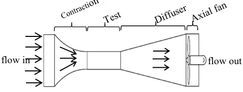
Wind tunnel has several spaces with their respective functions. Broadly speaking, each space has interrelated functions that are to maintain the uniformity of air flow into the test chamber and out of the test chamber. Thus the level of turbulence in the test chamber as long as there is no specimen will be removed. The creation of wind flow uniformity in the test chamber is the most important thing to be gained in the design and construction of wind tunnel [34]. Figure 2 shows the main components of a wind tunnel consisting of a contraction section, a test section and a diffuser section. Contraction section is the most important part in designing the wind tunnel; the resulting flow is very influential on the quality of flow in the test section.
Fig. 2. The suction type of open circuit wind tunnel
Before doing the design comprehensively then the first attention is done by determining the geometry dimension and the cross-sectional shape of the test chamber. The geometry dimension of the test chamber depends on the research object and the research objectives by using a wind tunnel. The quality of the measurements of the wind tunnel depends heavily on the quality of the airflow in the test chamber, then the air flow in the test chamber must be uniform, laminar moving, and the air velocity at each point is constant [37]. The geometry size of the test chamber that has been obtained is used to design and design another space according to the rules. However, in this study the first specified is the dimensions and inlet form, and the length of the contraction section. The inlet shape is varied with the dimension of the geometry of the contraction shape. The material for wind tunnel construction is a combination of acrylic and metal plate. Acrylic is used in the test chamber, while in other chamber use metal plate with thickness 3 mm. The purpose of the use of acrylic in the test chamber is to reduce friction between the wind flow and the acrylic surface, avoiding the potential for increased boundary layers. Acrylic has a type heat at 77 oF temperature is 1470
174005-1706-3838-IJMME-IJENS © October 2017 IJENS I J E N S
J/Kg-K and the possibility of deformation is negligible because it allows acrylic to be used up to 200 oF (93 oC).
A. Contraction Section
The criteria to be achieved in the design of contraction chambers for open circuit wind tunnel is the dimension of space geometry of minimal contraction to save space and the potential thickness of the boundary layer is minimal so as to avoid creating separation flow. The Non-Parametric Regression (NPR) method or surrogate method is then selected as a temporary model to obtain the size and design dimension that will meet the criteria while addressing the problem. After obtaining the optimal design then the dimensional points are processed to obtain a uniform flow pattern inside the chamber and find out using the CFD method [23]. The length dimension of the nozzle out the contraction space correlates linearly to the possibility of creating a boundary layer. In contrast, in contrast room design, the slope of the contraction-shaped curved wall space must be considered because it produces an adverse pressure gradient area so that a boundary layer separation is formed and then impacts the quality of the incoming wind into the test chamber. This means it is necessary to combine the effects of increasing the favorable pressure gradient by reducing the length of the contraction space [38].
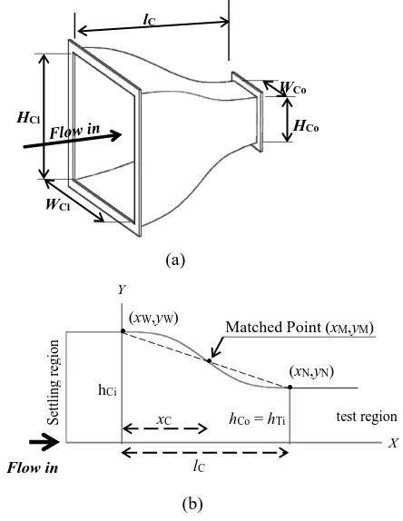
One such contraction space design as shown in Fig. 3 with the contraction form is determined by Equation 1 which is a 5th polynomial equation [39]. The point on the y-axis is obtained from the high difference of the input space contraction hCi to the high input difference with the hco output
height of the contraction chamber itself and the ratio between the curvature lengths of the input space xc contraction with the
total contraction length space lC. The hCi and hCo values are
half of the input space of the contraction and the contraction space outputs of HCi and HCo. The form of contraction by
using polynomial of order 5th is a moderate form compared to others. Polynomials under the order of 5 will make the contraction's output space increase in length, while above the order of 5 will shorten the length of the contraction space output. This will certainly affect the uniformity of flow out of the contraction space output and enter the test chamber.
Fig. 3. (a) 3D contraction section sketch; (b) a half 2D contraction section sketch
Figure 3b shows how to determine the center of the curvature of the contraction space form. The condition required to determine the initial polynomial is the coordinate (xw, yw) is at the input of the contraction space with the point
xM, yM is the center point of curvature. The horizontal
tangential condition at that point (xM, yM), the point at which
the contour line intersects the straight line is considered a control line, is set to half the length of the control line and intersect at that point. The control line starts from the starting point (xN, yN), with the same horizontal tangential conditions
at this point, and ends at the point xw, yw.
The polynomial formula used to determine the coordinates of contraction is shown in Equation 1. The contraction space curvature is also designed using the Logarithmic Derivative Profile (LDP) method as seen in Equation 2 also known as the Boerger model [21].
yC= ℎCi− (ℎCi− ℎCo) [6 (
xC
𝑙C)
5
− 15 (xC
𝑙C)
4
+ 10 (xC
𝑙C)
3
] (1)
yC= ℎCi+
(ℎCi− ℎco)
𝑙𝐶 𝑥𝐶[ln (
(ℎCi− ℎCo)
𝑙𝐶 𝑥𝐶)
− ln(ℎCi− ℎCo) + 1]
(2) HCo
HCi
WCo
WCi
lC
(a)
S
et
tl
in
g
r
eg
io
n
• •
•
test region
(xW,yW)
Matched Point (xM,yM)
(xN,yN)
hCi
hCo = hTi
lC xC Y
X
Flow in
Because of the symmetrical shape of the design, the variables that control the form of contraction chamber is inlet size, contraction length of space, contraction ratio and contraction chamber curvature.
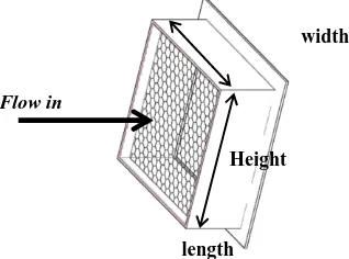
Settling chamber is part of an open circuit wind tunnel that is placed at the beginning of the circuit. When requiring high quality airflow, a device must be installed to increase uniform flow and reduce the turbulent level in the flow before entering the contraction section. Components mounted in the settling chamber of honeycombs that serves to straighten the flow as shown in Figure 4. The construction of this space is strung from thin plates with a thickness of 3 mm to ensure the strength and durability of space structures.
Fig. 4. Settling section with honeycomb
B. Test Section
Test section is a testing ground for a specimen as shown in Figure 5. The low level of air flow turbulence that goes into this test section is needed, the lower it will be better and more accurate for the simulation results of the test. The size for this test section depends on the test specimen to be tested in the wind tunnel.
Fig. 5. Test section C. Diffuser
The main function of the diffuser as shown in Figure 6a is to restore static pressure in order to increase efficiency and close off the circuit flow. The location of the diffuser is located after the test section and at the end of the diffuser will
be placed axial fan. If the length and diameter of the test section are given according to the design requirement, the length of the diffuser section depends on two variables i.e. the first variable is the test section diameter and the second is the Area Ratio (AR) of the diffuser section and defined by the designer. Therefore, the length for the diffuser section follows the formulation shown in Figure 6b.
Fig. 6. Sketch of diffuser section: (a) 3D shape (b) A half 2D shape
Fig. 7. 2D wind tunnel
Area Ratio (AR) is the ratio of the width of the inlet diffuser or outlet test section with the diffuser outlet shown in Equation 3. The AR value is determined by the designer as the independent variable and is equivalent to the angle of inclination in the diffuser (θ), where AR is the ratio of the inlet area and Outlet diffuser, A3 is area 3 (m2), and A4 is area
of 4 (m2)
Flow in
Height
length
width
Flow in HTin HTout
WTin WTout
HDin WDin
flow in
lD
flow out
(a)
L α R3
R4
(b)
Control Volume 4
Area 2
Control Volume 2 Control Volume 3 CR
Axial fan AR
α rNozzle
rEntrance
rTS
174005-1706-3838-IJMME-IJENS © October 2017 IJENS I J E N S
AR =A4
A3 (3)
By determining the equivalent cone angle for the diffuser nozzle, the length of the diffuser can be calculated according to Figure 6b and is calculated according to Equation 4, where L is the length of the diffuser (m), R4 is the radius of the
diffuser outlet (m), R3 is the inlet diffuser (m), and θ the angle
of the diffuser.
𝐿 =𝑅4−𝑅3
tan 𝛼 (4)
III. OPTIMIZATION METHOD
The design in this research using Ullman method is building some designs with TEA (Task Episode Accumulation) model. Designs constructed from different shapes and dimensions, visualized, until a variant comes close to the criterion of the designer [40]. The first stage is done by determining the range of measurement of the length of the side of the test chamber between 0.60 m 0.80 m, then entering the design phase of the contraction space that is set to have a length of 0.90 m for the reason of making the room effective. There are variations of length in the test chamber that is 0.50 m, 0.60 m, 0.70 m, 0.75 m, and 0.80 m. Each cross-sectional dimension of the test chamber produces the contraction space pair with its own dimension. Axial Fan Pulley used with a diameter of 1.250 m has a flow capacity is 8.75 m3/s. The design is done by varying the dimensions of
contraction, test section, diffuser. Variations of wind tunnel designs are shown in Table 1. The design chosen is the most optimal design in approaching the desired wind speed and turbulence intensity criteria.
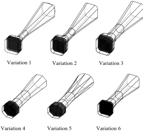
Diffuser design is given special attention to the diameter of curvature on the sides of the wind tunnel by following the design of the cross-sectional shape of the square. Different things with variant 4 and variant 5 have different cross-sectional shape each of which is octagonal with variant 5 followed by diffuser output form following fan shape i.e. circle. Attention is also given to the test section following the diffuser design pattern.
TABLE I
DESIGN VARIATIONS OF SETTLING CHAMBER, CONTRACTION, TEST SECTION, AND DIFFUSER
Var 1 Var 2 Var 3 Var 4 Var 5 Var 6
Diffuser (5°)
Fillet rectangular
d=400 mm Fillet rectangu lar d=500 mm Fillet rectangu lar d=500 mm Octagon al Octagon al & circle Fillet rectangu lar d=250 mm Dimensi
on (mm) 1250 1250 1250 1250 1250 1250
Test section Fillet rectangular 200 mm Fillet rectangu lar 250 mm
Fillet rectangu lar 250 mm Octagon al Octagon al Fillet rectangu lar 250 mm
Dimensi
on (mm) 500 x 500
600 x 600
700 x 700
800 x 800
700 x 700
750 x 750
Contrac tion
Fillet rectangular
d=400 mm Fillet rectangu lar d=500 mm Fillet rectangu lar d=500 mm Octagon al Octagon al Fillet rectangu lar d=500 mm Contrac
tion co-ordinat form
Dimensi
on (mm) 1250 1250 1250 1250 1250 1250
While in contraction design there are variations of form apart from dimension variation. Variation 1 to Variation 3 has a surface shape determined by Equation 1 in polynomial form, while the remainder is determined by Equation 2 in the form of a logarithmic equation. The last three forms of contraction design (Variation 4, Variation 5, and Variation 6) are then referred to as bell forms. The diffuser of the six designs is formed with the angle of inclination (θ = 5°) to the test section output and the maximum taken from the limit is (3° ≤ 2θ ≤ 10°) to obtain the diffuser length not exceeding 3.5 m so that the maximum space usage [35]. The boundary and cross-section are a fan diameter of 1.250 m. In the 1st variant, the test section and contraction are given a fillet with a diameter of 0.40 m to avoid turbulence due to edge currents. Square-sized sectional (0.50 x 0.50) m in the test section of variant 1, cross-sectional contraction section sized (1.250x1.250)m. Variant 2 has a cross section of the test chamber sized (0.60x0.60) m with angles filled with 0.50 m diameter fillets, the contraction sectional dimension still in the variant 1. Variant 3 has a contraction design that is still similar to variant 1 and variant 2 but the cross-sectional dimension the test chamber is (0.70x0.70) m, the design of the diffuser is unchanged with a slope angle made constant of 5° and its cross section is square with a fan diameter reference of 1250 mm. The sides are still given a fillet with a diameter of 0.50 m. Variant 3 has the shape of contraction space still resembles 2 previous variants, convex out on the input space and concave into the output. In the test section of the 4-sized variant (0.80x0.80) m has an octagonal cross-sectional shape, on its ribs which is a chamfer encounter of 0.25 m. Following the pattern of the test chamber, the cross-sectional shape of the contraction or diffuser is octagonal. In contrast to the shape of the previous contraction space, the contraction space in the variant 4 has changed shape. It is no longer formed from the polynomial equation but from the LDP equation so its shape becomes like a bell, formed only from a curvature that is curved into. The diffuser pattern does not change with the 5o slope following the form from the previous variants.
of 1.250 m. The cross section of the variant 5 is octagonal, still similar to the cross section of the 4th variant, with curvature pointing inward. Variation 6 has a contraction form similar to the 4 and 5 variants that are concave even though the size of the test chamber has been changed i.e. (0.75x0.75) m, but the dimensions of the contraction space remain at (1.245x1.245) m. Changes experienced in variant 6 are the provision of fillets at the sides meeting or ribs with a 0.50 m fillet diameter. The diffuser output gap following the 5 variant is made like a fan form with a diameter of 1.250 m although the angle of the diffuser still remains constant at 5°. Thus the designed variation, varying the cross-sectional dimension by the method of obtaining the cross-sectional shape, has been considered to meet the various parameters that will meet the need for wind tunnels as a means of developing aerodynamic research and fluid mechanics.
IV. RESULTS AND DISCUSSION
The first stage applied in the design of this type of wind tunnel is to eliminate sharp corners at each wind tunnel wall meeting to anticipate the formation of vortex and to get smooth flow transition near the wall and between hubs of each chamber. Vortex at an angle affects the pressure distribution in the output contraction section [21]. Numerical calculations yield three parameters: velocity v, pressure p, and Reynolds number Re are shown in the table according to predetermined variations.
A. Analytical Result
Starting with compute the inlet area of contraction chamber for calculates the flow inside another chamber where the length of the lc contraction space is 0.9 m, and applies both to
the polynomial and the LDP method. The geometry parameter in the first variation is for the contraction ratio of 6.8 obtained ratio (xC / lC) = 0.000, 0.111, 0.222, 0.333, 0.444, 0.556,
0.667, 0.778, 0.889, 1.000. Similarly, the same ratio was obtained for variations 2 and 3 with a contraction ratio of 4.7 and 3.3. While the last 3 models, contraction ratios are 2.2, 3.1, and 2.8, respectively, with space geometry obtained using LDP method.
TABLE II
DATA OF DESIGN RESULT AND CALCULATION OF EACH VARIATION
Data
Area 2
(Contraction)
Area 3
(Test section)
Area 4
(Diffuser)
V
a
ri
a
ti
o
n
1
A (m2) 1.466 0.216 1.466 P (kPa) 101.304 100.356 101.304
v (m/s) 5.967 40.584 5.967
L (m) 0.900 1.000 4.143
Re 462182 1283020 462182
V
a
ri
a
ti
o
n
2
A (m2) 1.447 0.306 1.447 P (kPa) 101.303 100.845 101.303
v (m/s) 6.048 28.555 6.048
L (m) 0.900 1.200 3.572
Re 468342 1083263 468342
V
a
ri
a
ti
o
n
3
A (m2) 1.447 0.436 1.447
P (kPa) 101.304 101.089 101.304
v (m/s) 6.047 20.049 6.047
L (m) 0.900 1.4 3.572
Re
(inlet) 468342 887354 468342
V
a
ri
a
ti
o
n
4
A (m2) 1.243 0.530 1.179
P (kPa) 101.296 101.165 101.293
v (m/s) 7.039 16.503 7.421
L (m) 0.900 1.4 2.43
Re 545157 834771 574792
V
a
ri
a
ti
o
n
5
A (m2) 0.977 0.406 1.243
P (kPa) 101.278 101.052 101.296
v (m/s) 8.956 21.555 7.039
L (m) 0.900 1.4 3.0
Re 614933 954024 545157
V
a
ri
a
ti
o
n
6
A (m2) 1.447 0.509 1.447
P (kPa) 101.304 101.151 101.304
v (m/s) 6.047 17.193 6.047
L (m) 0.900 1.4 2.715
Re 468342 815298 468342
174005-1706-3838-IJMME-IJENS © October 2017 IJENS I J E N S
size of the test chamber as shown in Table 1, except variation 1 is given curvature on its side with a diameter of 0.40 m as an alternative to the curvature design of the maximum curvature estimate will be applied to the design of this wind tunnel i.e. 0.50 m diameter. The diameter range of curvature between 0.40 m to 0.50 m provides a moderate cross-section, not producing a rounded cross section but providing a space that accommodates the parallel plate form as desired from the design. The size of curvature takes only ¼ part of each side plane. Curvature on the side is only intended to reduce and even eliminate the possibility of the emergence of vortices on the edge.
Fig. 8. Some variations from design wind tunnel; Variation 1, Variation 2, Variation 3, Variation 4, Variation 5, Variation 6.
The results of the design and calculation of wind tunnels that have a similar shape in Table 2, namely the velocity of flow in each space of each variant namely Variation 1, Variation 2, Variation 3 and Variation 6 then obtained the same tendency that the flow rate will increase with shrinking cross-section of space in its path. Although it involves Variation 4 and Variation 5 which has octagonal-sectional geometry, the same result is also obtained that the velocity will increase in the test chamber with a small cross-sectional area. That way the cross-sectional design of the wind flow does not affect the size of the speed, but is influenced by the geometry of the cross section. Variations in velocity dependent on the cross-sectional area are not only shown by the test section, the same pattern is shown in the contraction chamber. The data of the contraction section velocity of Table 2 obtained the maximum velocity in the contraction chamber owned by Variation 5 which has a cross-sectional area of 0.977 m2. The velocity of the smallest contraction section is
in Variation 1 which is 5.967 m.s-1 with the cross-sectional
area is 1.466 m2.
Fig. 9. Comparison of velocity in contraction section
The comparison of the flow velocity in the contraction section (Figure 9) between design and simulation shows the same trend in which Variation 5 has a top speed of 10.33 m.s -1, to simulation. As for the design result, the flow velocity is
8.956 m.s-1. The moderate velocities shown by Variation 4
and Variation 6 are 8.449 m.s-1 and 7.714 m.s-1 for the
simulation results then for the design results respectively are 7.039 m.s-1 and 6.047 m.s-1. Variation 1, Variation 2,
Variation 3 shows the price of the speed which is not much different, either from the simulation results as well as the design result.
Fig. 10. Velocity comparison in area test section
Figure 10 presents the sixth variance flow velocity ratio in the test section between the design results and the simulation results. The flow velocity in the test section tends to decrease with a negative gradient value except in Variation 5 showing an increase of 5.006 m.s-1 ,to simulation speed and 5.052 m.s -1 for the speed of the design result. Then Variation 4 and
Variation 6 show the design speed of 16.503 m.s-1 and 17.193
m.s-1 in the test chamber and the simulation results are 16.374
5.967 6.047 6.047 7.039
8.956
6.047
6.664 6.623 6.532 8.449
10.330
7.714
2.000 4.000 6.000 8.000 10.000 12.000
V
e
loci
ty
(m
/s
)
Design Simulation
40.563
28.555
20.049 16.503
21.555 17.193 43.750
29.749
21.151 16.374
21.380 18.088
5.000 15.000 25.000 35.000 45.000 55.000
V
e
loci
ty
(m
/s
)
Design Simulation
Variation 1 Variation 2 Variation 3
m.s-1 and 18.088 m.s-1. These results are the closest result of
the expected test flow velocity criteria about 15 m.s-1.
Fig. 11. Pressure comparison in test section
Figure 11 shows the sixth pressure curve of the variation in which the trend of the curve gradient is positive. However, if comparing the trend between the flow velocity curve and the pressure, both from the design and the simulation results, indicates nonconformity. The speed curve shows a negative trend. Pressure in the test chamber will increase when the area of the cross section is large, and this is the same for the pressure of the design result and the simulation result. But this condition can be understood that Variation 4 and Variation 6 has the smallest speed compared to other variations so that the small value of the speed affects the value of the pressure variation.
When the character of the design curve with the simulation curve shows the similarity of tendency as in Fig. 10 and Fig. 11, then different circumstances are represented by the speed curve of the diffuser. As shown in Figure 12, the flow velocity in the diffuser has a large difference between the simulation results and the design or numerical results in some variations. For example, variation 1 has a velocity difference in the diffuser of 3.746 m.s-1. Variation 2 produces velocity
difference of 2.714 m.s-1, Variation 3 produces velocity
difference that is 1.960 m.s-1, the velocity difference in
Variation 4 is 0.214 m.s-1. The velocity difference on
variation 5 is 0.791 m.s-1, Variation 6 yields a speed
difference of 1.163 m.s-1.
The difference is a consequence of the speed character used. The flow velocity in the design uses a scalar average speed, not the same as the flow rate in the simulation. The flow velocity at the simulation is the velocity of the velocity vector, the square root of the sum of the square of velocity in vectors i, j, k. This vector velocity is also influenced by different diffuser diffraction geometries due to fan adjustment.
Fig. 12. Velocity comparison on diffuser area
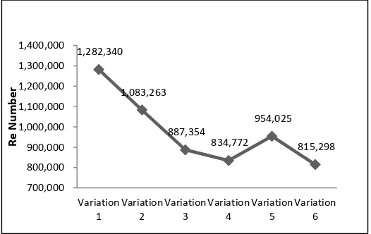
From the length of L data in Table 2, the optimal length of the tunnel is given by Variation 6 which is 5.015 m with Reynolds number in the test chamber is 815298 (8.2x10⁵).
This length includes the length of the contraction section 0.9 m, the length of the test section 1.4 m, and the length of the diffuser is 2.715 m. The shortest wind tunnel length is given by Variation 4 which is 4.73 m, but the Reynolds number value in test section of this variant is 834771 (8.3x10⁵).
As shown in Figure 13, since the Reynolds number is a function of the flow velocity the velocity curve pattern in the test section will be similar to the Reynolds number pattern in the test section. Taking into account the value of the Reynolds number, it can be assumed that the fluid flow in the wind tunnel is turbulent. Assuming that the flow in the wind tunnel is turbulent, it will be helpful in determining the maximum thickness of the plane boundary layer that may occur. Furthermore, the existence of separation flow can be predicted.
Fig. 13. Reynolds number in test section
B. Simulation Result
Figure 14 shows the flow velocity distribution within the wind tunnel along with the cross section wind section, with an
100.358 100.846
101.089 101.165
101.052 101.151
100.755100.795
101.070101.151101.055 101.134
100.200 100.400 100.600 100.800 101.000 101.200
P
re
ss
ur
e
(kP
a)
Design
Simulation
5.967 6.047 6.047
7.421 7.039 6.047 9.713
8.761
8.007 7.635 7.830 7.756
2.000 4.000 6.000 8.000 10.000 12.000
V
e
loci
ty
(m
/s
)
Design Simulation
1,282,340
1,083,263
887,354 834,772
954,025
815,298
700,000 800,000 900,000 1,000,000 1,100,000 1,200,000 1,300,000 1,400,000
Variation 1
Variation 2
Variation 3
Variation 4
Variation 5
Variation 6
Re
N
u
mb
e
174005-1706-3838-IJMME-IJENS © October 2017 IJENS I J E N S
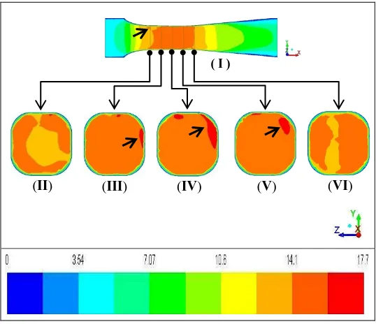
elongated extend (Fig. 14.I) and transverse at the bottom (Fig. 4.II -4.VI). Visual pattern of speed distribution in the wind tunnel is used to determine the most precise position of the test specimen in the tunnel, i.e. in areas with the most dominant flow uniformity. From the cross-sectional section of Figure 14, it can be concluded that the specimen should be placed in the middle between the plane III and the plane V because at that point the flow velocity and distribution of low inside test chamber is uniform and at the expected velocity value with the velocity of the region being 15.87 m.s-1. The
flow velocity changes as the speed increases as it enters the test section and then the speed decreases as it enters the diffuser. The smallest velocity is close to the wind tunnel wall and on the chamber settling, while the inlet contraction section has the same velocity at the diffuser outlet of 5.31 m.s-1 - 7.07 m.s-1. The price of speed obtained from the
analytical calculation is different from the simulation result because the speed obtained in the simulation is the average price of the velocity of the vector component while in the mathematical result, the speed value obtained is the value of the fluid velocity.
In a particular section of Figure 14 marked with arrows, refer to unstructured grid selection in simulation so there is an asymmetric flow distribution arises. Although the shape of the wind tunnel is symmetrical but to improve the accuracy of the modeling it is chosen unstructured grid. Figure 14.I appears a breakthrough speed below 15 m.s-1, and then at
cross section of Figure II-V near the wall there is a speed jump up to approximately 17 m.s-1. On Fig. 14-II, the visible
of velocity inside test chamber of wind tunnel not entirely uniform, as is the case in Fig. 14.III till Fig. 14.VI while Fig. 14.III – Fig.14.V shows the existence of speed up to 17 m/s. It is expected that the asymmetry fluid flow distribution inside the wind tunnel is not fully developed, so as not to disrupt the mainstream distribution nor aerodynamic tests are performed inside the tunnel.
This condition actually states that the uniformity of the flow in the test section is not pure even though the flow velocity difference appears on the side of a certain course and this does not take the whole portion of the test section. So this different part does not preclude the purpose of obtaining the position of the test object as a working area in the middle of the test section. Even the length of the specimen may exceed 0.30 m because the length of the space between planes III to plane V is 0.70 m.
This non-homogeneous velocity distribution originates from the outlet of contraction section and the cross-sectional section is at the corner so as to strengthen the vortices due to the turbulent corner boundary layer. But the small physical size of the boundary layer is difficult to determine the size of its thickness, especially if the boundary layer is the production of the cross flow factor [41]. The presence of boundary layer has no major effect on the test chamber and
other chamber due to the portion of the boundary layer thickness not significant. The increasing of boundary layer thickness can be seen in the diffuser and as saying before that it has no significant affect for uniformity flow inside test section.. Therefore further research on the character of the turbulent boundary layer corner needs to be done.
Fig. 14. Velocity contour at test section in m.s-1 unit
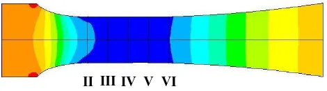
The speed of wind flow along the wind tunnel (x-axis) see at the visual velocity of Figure 14 can be observed in Figure 15, which represents the velocity at each point along the x-axis of the wind tunnel. The lowest wind speed at point 0 is the inlet contraction section and has a price that is almost equal to the point 500 m i.e. the point of outlet diffuser, between (6.0 - 7.0) m.s-1 while the point 200 m is the point
with a maximum speed of 15.0 m.s-1. The varied picture is
given by Figure 16 on the velocity graph although in the test region, the intensity of turbulence values obtained is quite constant.
(III)
(II) (IV) (V) (VI)
Fig. 15. Velocity distribution in wind tunnel (m.s-1)
For Turbulence Intensity along the center line of the x-axis can be seen in Figure 16 with a dotted line box marking the test section area. The magnitude of turbulence intensity in the test section of the region is in the range of 10.25% - 10.75%. From the picture, the wind flow has constant turbulence intensity while in the middle of the wind tunnel, with a high intensity in the test room input and the decreasing intensity at the test room output. These results are better than those done by Michalcová et. al. [42], [43] which approximately 11.0% by removing sharp corners in the wind tunnel.
Fig. 16. Turbulence intensity of wind tunnel in % unit
Fig. 17.Pressure distribution inside wind tunnel
One of the other parameters to determine the position of the test sample in the test chamber is the presence of visual data of pressure distribution as shown in Fig. 17. The apparent
color contours from simulation conclude that the highest pressure occurs in the conditioning chamber and part of the contraction area. The pressure slowly decreases as the fluid moves into the test chamber, and returns to its initial state gradually as it enters the diffusion chamber. This fact is contrary to the visual velocity showing the orange gradations in the test chamber as the maximal magnitude of the fluid velocity achieved. This condition is due to the increase of correlation rate with the increasing of fluid mass rate each time so as to reduce the mass density between the fluid particles. The interaction between particles against normal passage walls is reduced. The pressure of model in the test chamber obtained is -230.2 Pa.
The pressure distribution data (Fig. 17) shows the dominant blue gradation in the test chamber from the cross-section II to the VI cross section, except the II cross-section shows there is still a bright blue breakthrough indicating that the pressure at cross section II has not reached the point Minimal. Pressure in the cross-sectional area II is not entirely homogenous so positioning the test specimen in the cross-sectional area will not be optimal because the non-uniform pressure in the test chamber is one of the disturbances, except in the area between cross section III and section VI. These results confirm the results of the speed distribution shown earlier
V. CONCLUSIONS
This research presents about wind tunnel design optimization with several different methods such as Ullman method in determining design variation while tunnel geometry design using Polynomial Method and Logarithmic Derivative Profile method. The most optimal design is shown by the Variation 6 wind tunnel with a length of l = 5.015 m with the velocity in the test section is 15.0 m.s-1 with the
Reynolds number being 8.1x10⁵ and the turbulence intensity
of the region's test section is in the range of 10.25% - 10.75%. The flow velocity distribution inside the wind tunnel of the test specimen should be placed in the middle between plane III and plane V because at that region the flow velocity is uniform.
ACKNOWLEDGEMENT
This research was sponsored by The University's Applied Superior Research Grant with SP DIPA-042.06.1.401516 / 2017 from the Directorate General for Research and Development - Ministry of Research, Technology and Higher Education of the Republic of Indonesia.
REFERENCES
[1] C. L. Bottasso, F. Campagnolo, and V. Petrovi, “Journal of Wind Engineering Wind tunnel testing of scaled wind turbine models : Beyond aerodynamics,” vol. 127, pp. 11–28, 2014.
test section region
174005-1706-3838-IJMME-IJENS © October 2017 IJENS I J E N S
[2] V. A. Reyes, F. Z. Sierra-espinosa, S. L. Moya, and F. Carrillo, “Flow field obtained by PIV technique for a scaled building-wind tower model in a wind tunnel,” Energy Build., vol. 107, pp. 424–433, 2015. [3] B. J. Abu-Ghannam and R. Shaw, “Natural Transition of Boundary
Layers−The Effects of Turbulence, Pressure Gradient, and Flow History,”J. Mech. Eng. Sci., p. 213, 1980.
[4] J. M. Rainbird, J. Peiró, and J. M. R. Graham, “Journal of Wind Engineering Blockage-tolerant wind tunnel measurements for a NACA 0012 at high angles of attack,” Jnl. Wind Eng. Ind. Aerodyn., vol. 145, pp. 209–218, 2015.
[5] M. G. Silva and V. O. R. Gamarra, “Control of Reynolds number in a high speed wind tunnel,” J. Aerosp. Technol. Manag., pp. 69–77, 2009.
[6] L. Gao, Y. Liu, and H. Hu, “An Experimental Study on Icing Physics for Wind Turbine Icing Mitigation,” no. January, pp. 1–16, 2017. [7] A. Cezar, C. Ioan, A. Mugur, M. Degeratu, and R. Mircea, “Wind
tunnel and numerical modeling of atmospheric boundary layer flow over Bolund Island,” vol. 85, no. November 2015, pp. 603–611, 2016. [8] L. Yi, X. Changchuan, Y. Chao, and C. Jialin, “Gust response analysis
and wind tunnel test for a high-aspect ratio wing,” Chinese J. Aeronaut., vol. 29, no. 1, pp. 91–103, 2016.
[9] T. Maeda, Y. Kamada, J. Murata, M. Yamamoto, T. Ogasawara, K. Shimizu, and T. Kogaki, “Study on power performance for straight-bladed vertical axis wind turbine by field and wind tunnel test,” Renew. Energy, vol. 90, pp. 291–300, 2016.
[10] L. Zhang, Y. Feng, Q. Meng, and Y. Zhang, “Experimental study on the building evaporative cooling by using the Climatic Wind Tunnel,” Energy Build., vol. 104, pp. 360–368, 2015.
[11] W. Xie, P. Zeng, and L. Lei, “Wind tunnel experiments for innovative pitch regulated blade of horizontal axis wind turbine,” Energy, vol. 91, pp. 1070–1080, 2015.
[12] L. Mitulet, G. Oprina, R. Chihaia, S. Nicolaie, A. Nedelcu, and M. Popescu, “Wind Tunnel Testing for a New Experimental Model of Counter- Rotating Wind Turbine,” Procedia Eng., vol. 100, pp. 1141– 1149, 2015.
[13] G. V. Iungo, “Experimental characterization of wind turbine wakes : Wind tunnel tests and wind LiDAR measurements,” Jnl. Wind Eng. Ind. Aerodyn., vol. 149, pp. 35–39, 2016.
[14] Y. Chen, P. Liu, Z. Tang, and H. Guo, “Wind tunnel tests of stratospheric airship counter rotating propellers,” Theor. Appl. Mech. Lett., vol. 5, no. 1, pp. 58–61, 2015.
[15] M. Raimundo, R. Gaspar, A. V. M. Oliveira, and D. A. Quintela, “Wind tunnel measurements and numerical simulations of water evaporation in forced convection air flow,” Int. J. Therm. Sci., vol. 86, pp. 28–40, 2014.
[16] S. Liang, L. Zou, D. Wang, and H. Cao, “Investigation on wind tunnel tests of a full aeroelastic model of electrical transmission tower-line system,” Eng. Struct., vol. 85, pp. 63–72, 2015.
[17] Q. Xie, Q. Sun, Z. Guan, and Y. Zhou, “Journal of Wind Engineering Wind tunnel test on global drag coef fi cients of multi-bundled conductors,” Jnl. Wind Eng. Ind. Aerodyn., vol. 120, pp. 9–18, 2013. [18] T. Cho and C. Kim, “Wind tunnel test for the NREL phase VI rotor
with 2 m diameter,” Renew. Energy, vol. 65, pp. 265–274, 2014. [19] P. BRADSHAW and R. C. PANKHURST, “THE DESIGN OF
LOW-SPEED WIND TUNNELS.” National Physical Laboratory, Teddington, Teddington.
[20] M. Arifuzzaman and M. Mashud, “Design Construction and Performance Test of a Low Cost Subsonic Wind Tunnel,” IOSR J. Eng., vol. 2, no. 10, pp. 83–92, 2012.
[21] M. Rodríguez, J. Manuel, F. Oro, M. G. Vega, E. B. Marigorta, and C. S. Morros, “Journal of Wind Engineering Novel design and experimental validation of a contraction nozzle for aerodynamic measurements in a subsonic wind tunnel,” Jnl. Wind Eng. Ind. Aerodyn., vol. 118, pp. 35–43, 2013.
[22] D. E. Ahmed and E. M. Eljack, “OPTIMIZATION OF MODEL WIND - TUNNEL CONTRACTION USING CFD,” in 10th International Conference on Heat Transfer, Fluid Mechanics and Thermodynamics, 2014, no. July, pp. 87–92, 2014.
[23] A. S. Abdelhamed, Y. E. Yassen, and M. M. Elsakka, “Design optimization of three dimensional geometry of wind tunnel contraction,” Ain Shams Eng. J., vol. 6, no. 1, pp. 281–288, 2015.
[24] Ismail, S. Kamal, S. Tampubolon, A. A. Azmi, and Inderanata, “Modification of open circuit wind tunnel,” J. Eng. Appl. Sci., vol. 10, no. 18, pp. 8150–8156,
[25] J. K. Calautit and B. R. Hughes, “Wind tunnel and CFD study of the natural ventilation performance of a commercial multi-directional wind tower,” Build. Environ., vol. 80, pp. 71–83, 2014.
[26] M. D. S. Guzella, C. B. Maia, S. D. M. Hanriot, and L. Cabezas-Gómez, “Airflow CFD Modeling in the Test Section of a Low-Speed Wind Tunnel,” no. June, 2010.
[27] L. Leifsson and S. Koziel, “Simulation-driven design of low-speed wind tunnel contraction,” J. Comput. Sci., vol. 7, pp. 1–12, 2015. [28] T. Wang, “A brief review on wind turbine aerodynamics,” Theor.
Appl. Mech. Lett., vol. 2, no. 6, p. 62001, 2012.
[29] C. D. King, S. M. Ölçmen, and M. A. R. Sharif, “Computational Analysis of Diffuser Performance for Subsonic Aerodynamic Research Laboratory Wind Tunnel” Eng. Appl. Comput. Fluid Mech., vol. 7, no. 4, pp. 419–432, 2013.
[30] N. Q. Y, “Designing , Constructing , And Testing A Low – Speed Open – Jet Wind Tunnel Nguyen Quoc Y,” Int. J. Eng. Res. Appl., vol. 4, no. 1, pp. 243–246, 2014.
[31] T. H. Yong and S. S. Dol, “Design and Development of Low-Cost Wind Tunnel for Educational Purpose,” IOP Conf. Ser. Mater. Sci. Eng., vol. 12039, 2015.
[32] B. K. Bharath, “Design and Fabrication of a Supersonic Wind Tunnel,”Int. J. Eng. Appl. Sci., no. 5, pp. 103–107, 2015.
[33] M. K. Panda and A. K. Samanta, “Design of Low Cost Open Circuit Wind Tunnel – A Case Study,”,” Indian J. Sci. Technol., vol. 9, no. August, pp. 1–7, 2016.
[34] M. A. G. Hernández, A. I. M. López, A. A. Jarzabek, J. M. P. Perales, and Y. Wu, “Design Methodology for a Quick and Low-Cost Wind Tunnel,” in Wind Tunnel Designs and Their Diverse Engineering Application, InTech, pp. 3–28, 2013
[35] R. D. Mehta and P. Bradshaw, “Tehnical Notes of Design Rules for Small Low Speed Tunnels.”The Aeronautical Journal.
[36] M. Buckley and D. Sanford, “Low Cost Productivity Improvements in Low Speed Wind Tunnel Testing 20th AIAA Advanced Measurement and Ground Testing Technology Conference,” 1998.
[37] P. Moonen, B. Blocken, and J. Carmeliet, “Indicators for the evaluation of wind tunnel test section flow quality and application to a numerical closed-circuit wind tunnel,” J. Wind Eng. Ind. Aerodyn., vol. 95, no. 9–11, pp. 1289–1314, 2007.
[38] T. Morel,“Design of Two-Dimensional Wind Tunnel Contractions Design,” J. Fluids Eng., no. June 1977, pp. 371–377, 2013.
[39] J. H. Bell and R. D. Mehta, “Contraction Design for Small Low-Speed Wind Tunnels,” Jnl. Inst. Aeronaut. Acoust., no. April, 1988. [40] D. G. Ullman, “A model of the mechanical design process based on
empirical data,” Al EDAM, vol. 2, no. February, pp. 33–52, 1988. [41] Y. Su, “Flow Analysis and Design of Three-Dimensional Wind Tunnel
Contractions,” AIAA, vol. 29, no. 11, pp. 1912–1920, 1912.
[42] L. Leifsson, S. Koziel, F. Andrason, K. Magnusson, and A. Gylfason, “Numerical Optimization and Experimental Validation of a Low Speed Wind Tunnel Contraction,” in International Conference on Cmputational Science, 2012, vol. 9, pp. 822–831.