SLAM Based Autonomous Mobile Robot
Navigation using Stereo Vision
K. Al-Mutib
College of Computer and Information Sciences, King Saud University P. O. Box 51178, Kingdom of Saudi Arabia
Abstract - In this manuscript, we present an autonomous navigation of a mobile robot using SLAM, while relying on an active stereo vision. We show a framework of low-level software coding which is necessary when the vision is used for multiple purposes such as obstacle discovery. The system was implemented and tested on a mobile robot platform, and perform an experiment of autonomous navigation in an indoor environment.
Keywords - Stereo Vision, Localization SLAM, Mobile Robot.
1. Introduction
Stereo-vision based mobile robot navigation has always been a challenge. This is due to the complexity of integrating massive amount of information gathered by robot vision while it undergoes a motion. Visual perception of an environment, is also an important capability for mobile robots, and lots of efforts are being put by mobile robots research community. This is due to its consideration as a crucial part of mobile robot design.
1.1 Related Literature
In literature, there are considerable amount of efforts to let mobile robots to navigate visually within unknown, unstructured environments. In reference to Bonin-Font et. al. [1], they presented a substantial survey with a detailed summary of the most outstanding visual navigation studies from 1987 to late 1990s. Ghazouan et. al. [2] have also presented a new technique for model update using prior and current observations on the voxel state, they mentioned that; “environment is modeled using depth information provided by a stereo vision system”. Ghazouan et. al. [2] additionally mentioned that, “Workspace is decomposed into voxels which are the smallest volume of environment. A first observation on the state of the voxels is calculated based on stereo system provided 3D points and triangulation error propagation. The proposed update function uses a credibility value that denotes how strongly a new observation shall influence the voxel state based on the
age of the last observation and the homogeneity of the current observations”.
In [3], Guilherme and Avinash have collectively published a manuscript that surveys some developments over the last 20 years within the field of vision-based mobile robot navigation. They stated that, “For indoor robots in structured environments, we have dealt separately with the cases of geometrical and topological models of space. For unstructured environments, we have discussed the cases of navigation using optical flows, using methods from the appearance-based paradigm, and by recognition of specific objects in the environment”. ULUSOY [4] has presented an algorithm for active stereo vision, with depth perception for navigation. The algorithm was relying on SLAM routine for mobile navigation. On the other hand, a work initiated and applied by Fernando C. et. al. [5], was related to sequential EKF feature-based SLAM algorithm. Fernando C. et. al. [5] also stated that, “the features correspond to lines and corners -concave and convex- of the environment.
cheap but usually very crude, whereas a laser scanning system is active, accurate but slow. Vision systems are passive and of high resolution”. A concept of on-line trajectory generation for robot motion control systems enabling instantaneous reactions to unforeseen sensor events was proposed by Kroger [8]. Kroger [8] mentioned that “The paper presents the usage of time-variant motion constraints, such that low-level trajectory parameters can now abruptly be changed, and the system can react instantaneously within the same control cycle (typically one millisecond or less)”. Further Kroger [8] has added, “Such feature is important for instantaneous switching between state spaces and reference frames at sensor-dependent instants of time, and for the usage of the algorithm as a control sub-module in a hybrid switched robot motion control system “. Further referring were also reported Murray and James [9], and the formulated in the Carnegie Mellon University by Martin and Moravec [10] as approaches to figure out paradigm for internal representation of stationary defined environment, with an evenly spaced grids. That was based on ultrasonic range measurements.
In a wider context, occupancy grids also afford data structure that permits combination of sensor data. They also provide a representation of the environment which is created with inputs from mobile sensory devices. Apart from being used directly for sensory data fusion, there also exist interesting variations of evidence grids, such a s place-centric grids as in Youngblood et. al. [11]. Jia et. al. [12], have also presented a methodology related to map buildings while relying on interactive GUI (Graphical User Interface) for an indoor service mobile robot. This is due to the sensors uncertainty. Here, the operator can modify the map compared with the real-time video from the web camera of the mobile robot. Furthermore, for improving the robot precision for self-localization, EKF was also used.
An important research work literature related to mobile vision-based navigation also to be mentioned, is the one presented by Elfes, [13]. Elfes in [13], mentioned that “mobile motion were associated to the occupancy grid mapping, is the most widely used mobile robot mapping method. This is because of its simplicity, robustness, sufficiently flexible to be accommodated for numerous kinds of spatial sensors, with ability to be adapted very well towards non-stationary environments”. Nevertheless, range finders capture very slight properties of the real environment where a mobile robot is to move. They cannot acquire wealthy visual information that leads to the ultimate goal of humanlike perception of the real surroundings. Range finders are also limited by their successful measurable ranges, which depend on category and shape of the range finder being used. Consequently, within this article we shall be focusing on real-time stereo vision navigation. We shall explore implementation stages and present few navigation experimentation results. This includes; KSU-IMR architecture, system software and low level coding,
path searching, mapping technique with occupancy grids mapping, SLAM, Monte Carlo localization. To achieve the above mentioned navigation routines, the mobile robot was also fitted with advanced hardware computing resources. The robotic platform is to be capable of accommodating powerful computing, since visual data which is implemented by hundreds of millions of paralleling located units in the human eyes and brain, requires enormous computing power.
1.2 Study Purpose and Contributed Work
The purpose of this study is to realize an autonomous mobile robot navigation while relying entirely on active vision. Our algorithm is called H-SLAM (Hybrid-SLAM). This is because we have enhanced the SLAM with some supporting routines. We have developed an active vision system with a total of three degrees of freedom (pan, tilt, gaze) for each visual sensing. The stereo visual sensing is described first. After that, framework of the implementation is proposed. Next, the structure of the navigation software is further explained. This include the SLAM based stereo vision navigation. Finally, an indoor experimental results of the mobile robot is also illustrated. The implementation was achieved over a number of stages.
1.3 Paper Organization
The paper has been divided into six sections. In Section (1), we introduce related literature, background, and paper contribution . In Section (2), we present the overall mobile system architecture and related levels of hierarchy. Section (3) focuses on mobile robot vision and control hardware. Section (4), provides strategy of navigation. In section (5) we indicate a number of experimentations and results, thus verifying the proposed navigation methodology. Finally, in Section (6), discusses results and conclusion remakes are concluded.
2. Mobile Robot Hierarchy
2.1 Robot Hierarchy and Necessity
2.2 KSU-IMR System Architecture
In practice there are many tasks which are required to the active vision system sensor. Examples of which are: (i) Obstacle detection. (ii) Landmark extraction.
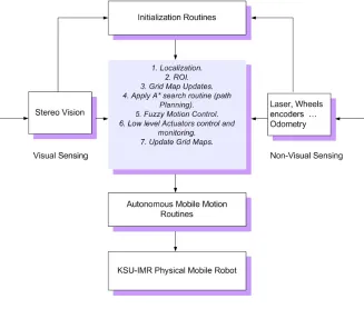
In reference to Fig. 1., KSU-IMR system architecture do consist of five fundamental blocks, (initialization, visual sensing, other sensing, navigation routines, and mobile body control).
Figure 1. KSU-IMR system hierarchy.
SLAM is used for state information and planning purposes.
2.3 Hierarchy Structure
The implementation approach is as follows: to design a mobile robotic system with stereo vision navigation capabilities. This is based on using visual data gathered from an environment. The mobile robot navigation design is to be based on a fundamental scheme; that high performance vision requires considerable computing strength. In order to fulfill this requirement, the proposed mobile robot was assembled to accommodate high performance computing power. An additional important tasks is the use of optimal path search based methods. Such a phase is achieved by creating navigation intelligence behaviors while robot is in motion. This will be based on intelligent techniques i.e. soft-computing techniques. Implementation phases are summarized as follows:
i. PHASE 1:
To perform modeling of different parts of the system. This includes different types of sensors, information provided by sensors and by cameras, fusion of data from sensors and acquired images, static and dynamic parts of an environments, mobile robot parts responsible for movements (e.g. wheels).
ii. PHASE 2. ROBOT BODY SELECTION:
To select an appropriate mobile robot body design, and to assemble the appropriate intelligence that helps the mobile system for an indoor navigation path planning. In addition, the research also includes a coding of system onboard intelligence.
2.3 Management of Plural Duties
In reference to Fig 2., we show the proposed mobile control system. The control is based on generating the most appropriate paths for mobile motion, whereas a SLAM has been also based used to incorporate and update the accurate adjustments. The figure also show how the environmental data have consequences the SLAM calculated feedback (mobile robot pose).
3. Active
Stereo
Vision
and
Motion
Hardware
3.1 Active Stereo Vision
Stereo vision is useful for mobile robots. It has a benefit in knowing the distance information or 3D shape of obstacles. It can also be used for landmark extraction for mobile robot self-localization. Two cameras are fixed on a platform whose pan, tilt, and gaze are
movable manually or from the computing hardware. A number of servo motors are employed for the camera head, for gaze, pan, and tilt control. The pan range of movement for each of upward and downward tilt movement ranges, is up to (±50°). Top level coding and multiple computers are used for performing the CPU rigorous tasks in real time using a distributed computing architecture. This is to be capable of dealing with large number of sensing and control signals, as shown Fig. 1. In reference to Fig. 1., we have shown KSU-IMR software and hardware hierarchies.
3.2 Mobile Robot Control Hardware
This phase involves an accommodation of main computing power of POWERROB robot boards. They are used for distributing computing actions to cope with the challenges from the real-time high computing power needs. Such a task also involves stereo vision and visual data processing. Other uses are, the master controller that handles all optimal path planning, controlling drive motors, and servo motors for moving camera platform. We have employed high current dual channel DC motor controller, this will be capable of handling high current, and give high movement toques.
4. Navigation Strategy
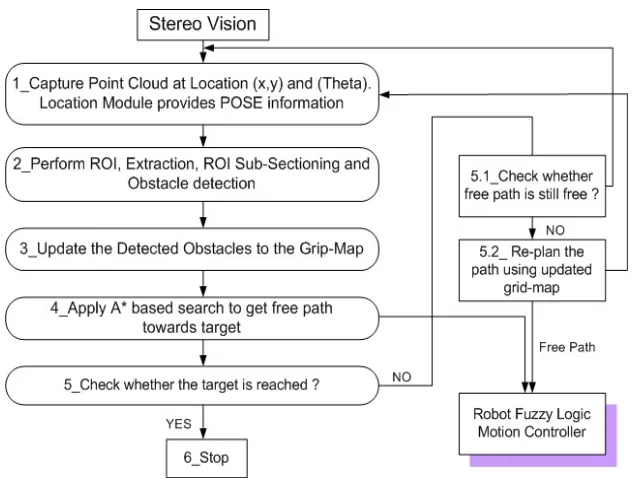
The drive behind this study is to realize an autonomous navigation of the mobile robot. Our environment is an indoor laboratory and corridors in the building. This is shown in Fig. (3). The in-depth structure of navigation software is shown in Fig. (4). Navigation software consists of “mobile robot navigation”, and “self-localization”. In reference to Fig. 4, we also show the overall coding hierarchy. It is an illustrations of the five fundamental stages of the stereo-vision navigation, including localization, ROI, grid mapping optimal path search via *
A , and path planning. We shall elaborate additional within the following sub-sections.
4.1 Coding Interconnected Units
Figure 3. Target environment of the navigation.
Five fundamental stages for stereo-vision navigation, (localization module, ROI, grid mapping updating, A* search, and path planning).
Another unique characteristics to be acquainted by the mobile robot, is the visual 3D perception that uses both depth from focus/defocus and the 3D binocular stereo. Building intelligence for mobile robot path planning. This is achieved by creating navigation intelligence capabilities while the robot is in motion. This is further based on intelligent path planning techniques (soft-computing methods). The four important units are (localization, map building and updating, searching optimal path planning, and motion control routine), as in Fig. 4.
4.2 Navigation Routines
4.2.1 Localization Routine
KSU-IMR localization at particular current time-step k, the intension is the estimating robot state. This is achieved as based on knowledge of mobile initial state in addition to initial measurements
(
)
{
z ,i 1, ,k}
Z k
k L
=
= up to current time. This is expressed in terms of mobile posture, the
(
x,y)
position and orientation( )
θ . By definition this is a three-dimensional state vector x=(
x,y,θ)
T. As stated earlier, we are integrating the vision localization techniques, hence we are laying down a heavy integration of these techniques into the developed SLAM routine.4.2.2 Mobile Optimal Path Searching: ( *
A Search)
For choosing mobile robot optimal path (shortest navigation path), *
A search algorithm has been used. Along its way, *
A search algorithm passes through a mapping graph, hence it surveys for the best path of the lowest known cost, while updating a sorted priority queue of different path divisions. In its basic principle, in a continuous search till a final goal is found, during a traversing a mobile detected map, a section of a path being traversed would be given a higher cost than another encountered path segment. It leaves the higher-cost path segment and continues to search for lower-cost path sections. In its straightforward principle, *
A relies on concept of best-first search, and finds a least-cost path from an assumed mobile robot initial posture to mobile goal posture. Denoting f
( )
x as a Distance-Plus-Cost heuristic function DPC, hence *A uses f
( )
x to decide a direction in which the search visits mobile posture in a tree. DPC is a summation of two parts. FIRST: A path-cost function. This is a cost from an initial mobile robot posture to a present one, g( )
x . SECOND: A "heuristic estimate" for the distance to mobile desired posture, as named by h( )
x . The h( )
xterm of f
( )
x function, must show an admissible heuristic; meaning that it must not overestimate the distance to the goal. For a use of the *A in mobile robot routing, function h
( )
x might be characterized by a straight-line distance to a ending mobile target position.Once the heuristic h
( )
x satisfies an additional condition( )
(
)
( )
(
h x ≤d x,y +h y)
for every edge(
x,y)
of the graph (where d denotes the length of that edge), in this respect, h( )
x is then to be consistent. For such a case,*
A can assume an effect implementation, i.e. no node needs to be processed more than once and *
A is equivalent to running Dijkstra's algorithm, however, with the reduced cost:
d′
(
x,y)
=(
d(
x,y)
−h( )
x +h( )
y)
(1) Though has such potentials, a main concern of the*
A search, is related to time complexity. This is in a total dependency on a heuristic search. This can be seen as an exponential expanding of mobile robot number of nodes, while storing information about a shortest path. However, for a tree traversing search, this is a polynomial. Since there is only a single goal posture, the mobile robot must move to, hence the heuristic function h
( )
x is to satisfy the following condition:h
( )
x−*h( )
x =O(
logh*( )
x)
(2)In Eq. (2),*h
( )
xis defined as an OPTIMAL HEURISTIC, i.e. the exact cost to get from location
( )
x to a final mobile robot target position. Equation (2) can be interrupted as follows: Heuristic error in h( )
x should not propagate faster than the logarithm of *h( )
x, the “BEST heuristic”, which computes an accurate distance from robot initial posture
( )
x to a targeted posture. In summary, *A relies on both, backward costs, and forward costs, i.e. “estimates of”. In its nature, it can be mentioned that, the *
A is optimal with admissible heuristics.
4.2.3 Mapping Technique (Occupancy Grids)
to be detected. Grid localities within these defined regions of ambiguities have their assigned values increased. On the contrary, localities within a sensing pathway, more precisely the ones between mobile robot and localities in the sensing path between the robot and the obstacle, will be assigned “reduced probabilities”. For constructing an occupancy grid, the visual sensing tool has to be correctly modeled. In this context, Murray and James [9] has indicated that, “our own experiments with sub-pixel interpolation indicate that the Triclops stereo vision module produces results with standard deviations well below one pixel”. In order to reduce sensing computational time, and real-time considerations, sub-pixel interpolation have not been used within this stereo algorithm. Hence, we can still approximate a model for the mobile robot stereo vision by adopting the following approximated relation of Eq. (3):
(
d|)
1P β = for β=β
(
d+0.5)
→β(
d−0.5)
(3)(
d|)
0P β = otherwise
Given the mobile vision system geometrical layout, for used stereo vision system, and while aligning optical axes with a focus at infinity, we defined a relation of disparity d to depth β as:
( )
γ ββ
=
d f
d (4)
In Eq. (4), γ is a baseline between two cameras, whereas d is the disparity. We need to shift from one dimensional vision to two dimensional. This is done via stereo triangulation technique. For each individual pixel resulting from a pair of cameras, stereo triangulation is therefore a result of intersection of the lines of sight.
Stereo triangulation technique is used to create a two dimensional position of an obstacle detected by the mobile robot. This is based on particular pixel (i)over an image of a reference camera, and resulting a disparity result (d) from stereo matching. Further analysis of lines of sight of the centers of two pixels, there is further an error bound, this is as a result of “diamond” shape around a position. It resembles an elliptical area used as a model in Matthies and Shafer [14]. In reference to geometry of triangulation, as in Guilherme et. al. [15], it is needed to evaluate for a given pixel and disparity a region of uncertainty. For the trapezoidal region of uncertainty corresponding corners are evaluated by calculating areaβ, whereβ=β
(
d±0.5)
.Hence calculating
(
)
±
=
f 5 . 0 x
X β . Here
( )
x is an image plane coordinate alongside image rows, in addition, a f is the focallength. An unoccupied area,for which an obstacle should notappear, is in reality a triangular as shaped by the robot’s posture, and the closest two corners of the trapezoid.
4.2.4 Mobile Robot SLAM Routine
(Mobile Simultaneous Location and Mapping)
Slam is considered as an important integral of autonomous mobile robot navigation. It represents an ability to place an autonomous mobile robot at an unfamiliar location in an unknown environment, and then have it figure a map, using only relative observation of the environment, and then to use this map simultaneously to navigate. The focal idea behind the SALM technique, it is an observation of robot motion from a starting unknown posture or vicinity while maneuvering within an environment. Furthermore, absolute features localities are not accessible. It is proposed to adopt linear evolution of motion as this results in robot synchronous discrete-time model and the observations of landmarks are known. It is known that robot motion and observation of features, the landmarks, are nonlinear while navigating, however, using linear models does not reduce the accuracy of the approach. In this regard, within this paper, we shall use nonlinear robot model in addition to nonlinear observation models. This includes system state, such as position and orientation of the robot, in addition to the position of landmarks. Denote the state of the KSU-IMR robot as Xij
( )
k . While maneuvering, the dynamical motion of the robot is modeled by linear discrete-time state transition equation, Eq. (5):
(
k 1)
F( ) ( )
k x k u(
k 1)
V(
k 1)
Xv + = v v + v + + v + (5) In Eq. (5),Fv( )
k is state transition matrix, uv( )
k is control input, and Vv( )
k is uncorrelated mobile dynamics noise errors, expressed with zero mean and covariance Qv( )
k .We shall name a locality of an ith feature (landmark), by
i
p . Refer to [xx] for further details. Defining state transition matrix of an ith observed feature as:
(
)
i( )
ii k 1 p k p
p + = = (6)
For the time being we shall let number of features as size N vector, and as stationary features. A vector of all N landmarks is given by:
(
T)
TN T
2 T
1 p p
p
p= L (7)
( )
(
( )
T)
T N T 1 N T 1 Tv k p p p
x k
x = L −
(8)
This leads to the following robot and features state transition dynamic model:
(
)
( )
( )
(
)
(
)
+ + + + = + − pN 2 p 1 p v pN 2 p 1 p v N 2 1 v pN 2 p 1 p v N 1 N 2 1 v O O O 1 k V O O O 1 k u p p p k x I 0 0 0 0 0 0 0 I 0 0 0 0 I 0 0 0 0 k F p p p p 1 k x M M M O M M M M L(
k 1)
F( ) ( )
k xk u(
k 1)
v(
k 1)
x + = + + + + (9)
In Eq. (9) Ipi is ( ) ( )pi×pi
ℜ identity matrix and matrix Op1 is dim(pi) null vector.
Motion Predication Phase.
In reference to robot named frames, for the case of iC as a vector of coordinates of ith defined landmark, where there are k landmarks, as state vector is hence defined as
(
( ) ( ) ( )
T)
Tt k T t 1 t xt ,yt, t,c , c
S = θ L . For the
PowerRob mobile robot system, it is equipped with
(
∆θR,∆θL)
, i.e. differential drive in which right and left angular displacement of wheels are known. For instant, if robot wheels rates considered contact during one sampling period, we can decide robot kinematics using the geometric models. This is expressed as: stop( )
( )
( )
( )
(
(
)
( )
)
(
)
(
(
)
( )
)
( )
+ − + − − + + = − − − − − − − θ ∆ θ θ θ ∆ θ θ ∆ ∆ θ θ ∆ θ θ ∆ ∆ θ 1 t 1 t 1 t 1 t 1 t 1 t 1 t cos cos L y sin sin L x t t y t x (10)In Eq. (10), the terms
(
∆L,∆θ)
are representing the “linear” and “angular” displacement of mobile robot. In terms of robot physical parameters, they are also expressed by:(
)
(
)
+ = + = l L L R R L L R R r r 2 r r L θ ∆ θ ∆ θ ∆ θ ∆ θ ∆ ∆ (11)MAP Model Updating Phase.
While building a MAP, this entirely dependent on voxels. However, we need to update states of each voxel by adopting
(
K( )i,t :0↔1)
, as a credibility value. In this sense, such a CREDIBILITY MEASURE defines a measure to trust a given observation O( )( )t Vi of voxel( )
i calculated based on the stereo pair taken at a time instant( )
t . Such a map update is computed based on time index consideration, i.e. for a defined time t, and for an updated occupancy observation O(t+1)( )
Vi , the corresponding voxel state is updated by Ghazouani et. Al. [16]: ( )( )
( )
(
)
( )
− + = + + + + 0 O k V S k 1 V S VS i,t1 t i i,t 1 t1
i to i 1 t (12)
In reference to Eq. (12), K( )i,t is depending on a number of time varying terms. Such a dependency does include determined voxel neighborhood homogeneity, quantity of preceding measurements, and period of last observation. Already occupied voxel is not likely to be found in an otherwise empty environment. Therefore, measurements demonstrating homogeneous sections, are further expected to be credible, and we don't want to trust the very first measurements and over aged measurement at a point too much. If O( )t
( )
Vi is designated as neighborhood homogeneity of an observation, hence O( )( )t Vi is found through by using set of( )
N voxel within neighborhood of( )
Vi . It is useful to only view the directly neighboring voxels.To achieve this, Eq. (13) expresses homogeneity of an observation at a voxel
( )
Vi at a time instant t:( )
( )
(
)
− =∑
∈ N V O V OVjN t i t j t
, i
Η (13)
( )it,
k in Eq. (12) is an credibility measure and is expressed in terms of homogeneity of an observation
( )it,
Η as in Eq. (14):
( ) ( )
(
( ))
(
)
− − − = o 2 last t , i t , i t , i t 2 t t exp 2 H 1 N k σ π (14)observation, as calculated for voxel V( )i and finally. σ is representing a constant for age scaling. Meta information (previous observations age, prior observations counts), are important data to be updated, such updates are stored in each voxel. For experimentation purposes, we shall show laboratory ground used for building maps. We shall show representation of states of voxels in a 3D scene for same testing laboratory ground.
4.2.5 Monte Carlo Localization
Monte Carlo stereo vision based Localization (MCL) has been used. It works as a primary layer for localization parameters estimation. In sampling-based methods we represent a
(
k)
k Z x
p M density by a set of
N random samples or particles S
{
si,i 1 N}
kk = = L
drawn from it. We are able to do this because of the essential duality between samples and density from which they are generated. From the samples, we can always approximately reconstruct the density while using a histogram or a kernel based density estimation technique. The objective is then to recursively compute at each time step k set of samples Sk that is drawn from
(
k)
k Z x
p M . A particularly elegant algorithm to
accomplish this has recently been suggested independently by various authors. It is known alternatively as the bootstrap filter, Gordon et. al. [17], the Monte-Carlo filter [17], even the condensation algorithm Gordon et. al. [17]. Such methods are generically known as particle filters, and an overview and discussion of their properties is found in Gordon et. al. [17]. In analogy with formal filtering formulation outlined in Section 2, the algorithm proceeds in two phases:
PREDICTION PHASE. In the first phase we start from a set of particlesS(k−1) computed in previous iteration,
and apply the motion model to each particle ( ) i
1 k S − by
sampling from the density
(
( ) (k1))
i1 k k|s ,u x
p − − : (i) for each
particle ( ) i
1 k
s − draw one sample ( ) i
k
s from
( ) ( )
(
k 1)
i 1 k k|s ,u x
p − − . Hence a new set of Slk is obtained that approximates a random sample from the predictive density
(
(k1))
k|Z
x
p −
. The prime in Slk indicates that we have not yet incorporated any sensor measurement at time k. In reference to [17], and to draw an approximately random sample from the exact predictive probability distribution function
(
(k1))
k|Z x
p −
, we use
motion model and set of particles S(k−1) to build an empirical predictive density function of :
( )
(
)
∑
(
( ) ( ))
= − − − = N 1 i 1 k i 1 k k 1 kk|Z px |s ,u x
p (15)
In Eq. (15), we describe a blended density approximation to
(
(k1))
k|Z x
p − . This is combining one
equally weighted mixture component
(
( ) (k1))
i1 k k|s ,u x
p − −
per sample ( ) i
1 k S − .
UPDATING PHASE. In the second phase we take into account measurement of zk and weight each of the
samples in Slk by the weight
(
)
i k l k ik pz |S
m = , i.e. the likelihood of ik
l
S given zk. We obtain Sk by resampling from this weighted set: (ii) for
(
1, ,N)
j= L : draw one
k
S sample j k
S from
{
i}
k i k l m , s .The resampling selects with higher probability samples i
k 0
S that have a high likelihood associated with them, and in doing so a new set of Sk is obtained that approximates a random sample from
(
k)
k|Z x
p . An
algorithm to perform this resampling process efficiently in O
( )
n time was presented by Gordon et. Al. [16]. After updating phase, two steps (i) and (ii) are repeated recursively. To initialize the filter, we start at time0
k= with a random sample
{ }
i 00 s
S = from the prior
( )
x0p . Over such a second phase, it is needed to use the mobile measurement model to acquire a sample l
k
S from the subsequent terms
(
k)
k|Z
x
p . Instead we shall be using definition given in Eq. (15), and to sample from the empirical posterior density:
( )
(
)
(
)
(
(k1))
k k k k
k|Z pz |x pˆ x |Z
x
p −
∝ (16) Monte Carlo Localization coding was achieved using
C++ layer, with linked libraries for onboard execution. Xxxxx
5. Implemenation and Results
5.1 Experimental Setup
The navigation strategy mentioned in previous section is implemented on an autonomous mobile robot “KSUMR”, and verified by the following navigation experiment in a real environment.
5.2Experimental Results
5.2.1 Localization Phase
proportional to distances traveled by the robot and the ODOMETERY/GYRO inaccuracies. A number of initial experimentation have indicated that, mobile posture uncertainty increased significantly at each time step.
Monte Carlo Localization: It was chosen to implement a stereo vision Monte Carlo Localization (MCL). It will serve as a primary layer for localization parameters estimation. To enhance the robustness to localization technique, we switch to Dead Reckoning localization whenever the MCL layer failed to localize the robot due to sensor noise or unpredictable robot motion. Monte Carlo Localization was chosen as primary “localization” method. This is because it is superior in terms of its computational cost, moreover it supports multi-modal location distribution. In other words, these distributions are in fact possible locations for a robot, estimated by a motion model. Multi-modal distribution support gives us an ability to take into account multiple motion
scenarios (e.g. either the robot is stationary, turning or moving straight). To validate the presented concepts, earlier presented Monte Carlo localization technique has been therefore widely tested in the laboratory ground office environment using diverse mobile robotic postures. Over a set of repeated experimentations, experimentations efforts have resulted and indicated that, such a technique is both efficient and robust. It was running comfortably in real-time. Verifying Monte Carlo localization, even under more challenging situations, the experiments described here are based on data recorded from the POWERROB mobile hardware. For localization, even though the sensory information were sensed and recorded at prior and previously defined time index, the time-stamps in the logs were used to recreate the real-time DataStream coming from the sensors. Hence, the obtained computational results are not conflicting with real data measured and collected from the mobile robot sensory instrumentation readings.
Iterative Closest Point Localization: As part of the development of MCL layer, we customized the standard stereovision based Iterative Closest Point (ICP) method to suit our environment and sensor configuration. The resultant algorithm is able to localize the mobile platform with an upper bound of
(
19cm)
with respect to translational localization. Upper bound for rotational motion was stood at(
o)
3 .
3 . Execution cost for this algorithm turns out to be very high and the robot translational speed has to be restricted at 50 mm/sec. The robot’s angular speed is restricted at a much slower
(
5o/sec)
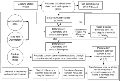
. Reasons for such upper bounds is the high computational load on the on-board PC. The flow chart for such employed (ICP) algorithm was already presented and detailed in Fig. 5.
5.2.2. Localization Sensor Fusion
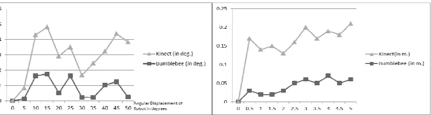
An effort was made into accumulating localization results from multiple vision sensors i.e. “Microsoft Kinect” and “Point Grey Bumblebee” for greater accuracy. Localization results deduced by experiments conducted on Microsoft Kinect and Point Grey Bumblebee camera suggested that Microsoft Kinect sensor has more inherent noise in depth value readings as compared to Bumble camera depth readings. In this respect, both of the results indicated to in Fig. 5 show positional error for mobile robot during localization process using each of the named sensors. Since Kinect sensor never performed better in any of the scenarios, the idea of combining localization results of both sensors was discarded. The research platform and experimental setup used in this experiment is shown in Fig. 6.
A grid-based mapping approach was selected for the implementation of SLAM algorithm. Among the primary concerns about mapping, the implementation ensured that real-time execution, map-accuracy via modeling un-certainty and loop-closure detection is well-implemented within the mapping module.
Grid-resolution for the evidence map was tested with
(
50mm)
,(
100mm)
and(
200mm)
resolutions. Accurate navigation and path-planning results were achieved.(
100mm)
resolution however, was chosen to be the consistent resolution upon which all future experiments would be conducted as it rendered the minimum cost in terms of execution time and navigation accuracy. The size of the map currently stands at(
2)
m 900 .
Until now there have been no experiments designed, that require a larger area than the mentioned figure. The mapping updates and initializations are restricted to the area under observation ,which roughly equals
(
2)
m
15 ,
thus any increase in map area will not trigger map-wide initialization or update. For map accuracy in terms of detection of small-sized obstacles and gradient floors, we have developed a customized algorithm and verify it over a number of experimentation trials. The verification results for running such an algorithm is presented in Fig. (7).
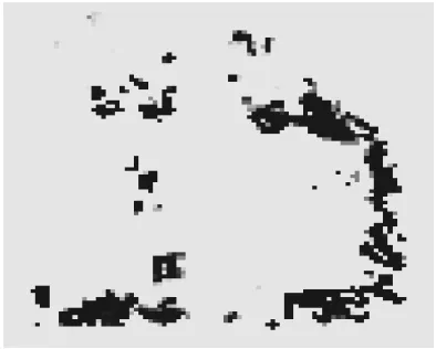
The implemented mapping module can detect a loop and propagate errors in previous poses. The grid-map cells store both the height data about the environment and also the certainty measure about the existence of an obstacle. The certainty is a function of two elements i.e. the amount of time an obstacle is observed within a cell and secondly the number of points returned by the sensor that lie within each cell. An example of a confidence map generated of obstacles in the environment (including loop detection routine) is represented in Fig. 8. Darker grid-cells represent a high probability of presence of an obstacle. Lighter shades represent an opposite hypothesis. Each observation is added to the map as a Bayesian update.
Figure 6. Experimental system setup. (Top)Results for voxels states representation using three stereo pairs taken from three different
positions of the stereo cameras. (Bottom)
The PowerBot system hardware configuration as made ready for localization experiments.
Figure 7. Results and verification of the mobile robot floor detection algorithm.
Figure 8. Map generated by in-place visual servoing (directed perception).
Figure 9. Path-planning over maps results.
5.2.3 Map Accumulation Algorithm
The criteria for adding an observation to the built map can be defined as follows: A Bayesian update will either increase or decrease the probability of presence of an obstacle within a cell, refer to Eq. (12). This probability depends upon following factors: (i) Presence of points lying in the cell within the current observation. (ii) Consecutive number of observations for which a minimum number of obstacle points can be associated to a grid-cell. This mechanism handles fast moving dynamic obstacles. (a) All cells occluded by obstacles are not updated. For this purpose only the
( )
o66 FOV in front of camera is considered for map updates. (b) The obstacle height data is only used for loop-closure detection. For obstacle detection, a combination of obstacle height and their persistence over multiple observations is employed.
5.2.4 Fast SLAM
Another layer based navigation approach was tested on the sidelines of this experimental bed. This approach presents a motion control for an autonomous robot navigation using fuzzy logic control. This requires the capability to maneuver in unstructured, dynamic and complex environment. The mobile robot uses intuitive fuzzy rules and is expected to reach a specific target or following a pre-specified trajectory while moving among unforeseen obstacles with the help of stereo-vision camera. The robot's execution depends on the choice of the task. In this approach, behavioral-based control architecture is adopted, and each local navigational task is analyzed in terms of primitive behaviors.
5.2.4 Fast SLAM Path-Planning
In reality, quite large of trails were successfully conducted exper imentally within complex indoor obstacle scenarios for path-planning using the developed version of the Fast SLAM. The mobile robot has successfully reached its target
(
x,y)
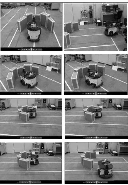
location using the planned paths in an autonomous approach. Furthermore, currently we submit a set of goals to our system, hence the system plans path in sections for each of the goal. Once an obstacle scenario is significantly changed so much, in such a way that it affects the planned path, *A algorithm is used to re-plan the path to the goal. The planning and re-planning delays are less than a time of a second long, so there exist no issues for performance degradation within path-planning module. Specifically, some of the path planning examples and runs, can be seen in Fig. 9. Finally both Fig. 10 and Fig. 11 show a demonstration part of intensive experimentation and verifying the real-time mobile navigation outcomes.
Figure 10. Video recording and shots, hence verifying mobile robot navigation without collisions.
Figure 11. Graphical (x,y) data recording and navigation verifications. (Top) Simple to target maneuvering, and motion to a posture path planning.
6. Conclusions
In this paper, we focused on the autonomous mobile robot navigation using the active stereo vision. We developed the navigation strategy as based on integration of a number of important navigation routines. Hence, we also propose a framework of the vision system with the software level, which mediates the plural sensing requests and manages the vision recourses. The mobile body was experimentally tested for full navigation within an unstructured dynamic environment. A real-time stereo-vision SLAM technique was employed for motion purposes. The mobile robot has shown an excellent model of integration amount different layers and unit.
References
[1] Bonin-Font F., Ortiz A., and Oliver G. (2008), Visual Navigation for Mobile Robots: A Survey, Journal of Intellignet Robotics Systems, 53: 263– 296.
[2] Ghazouan H., Tagina M., and Zapata R. (2010), Robot Navigation Map Building Using Stereo Vision Based 3D Occupancy Grid, Journal of Artificial Intelligence: Theory and Application, 1,3: 63-72. [3] Guilherme D. and Avinash K., (2002), Vision for
Mobile Robot Navigation: A Survey," IEEE Transactions on Pattern Analysis and Machine Intelliegcne, 24, 2 : 237-266.
[4] Ulusoy L. (2003), Active Stereo Vision: Depth Perception for Navigation, Environmental MAP Formation and Object Recognition, The Middle East Technical University, Tuerky.
[5] Fernando C., Natalia L., Carlos S., Fernando S., Fernando P., and Ricardo C., (2010), SLAM algorithm applied to robotics assistance for navigation in unknown environments, Journal of NeuroEngineering and Rehabilitation, 7,10 : 1-16. [6] Elfes A. (1989), Using occupancy grids for mobile
robot perception and navigation, IEEE tranasactions of Computer Magazine, 22, 6 :46–57.
[7] Stephen S., Lowe D., and Little J. (2002), Mobile Robot Localization and Mapping with Uncertainty using Scale-Invariant Visual Landmarks, International Journal of Robotics Research, 21, 8: 735-758.
[8] Kroger T. (2012), On-Line Trajectory Generation: Nonconstant Motion Constraints, IEEE International Conference on Robotics and Automation RiverCentre, Minnesota, USA :14-18.
[9] Murray D. and James L. (2000), Using Real-Time Stereo Vision for Mobile Robot Navigation, Journal of Autonomous Robots, 8 :161–171.
[10] Martin M. and Moravec H. (1996), Robot Evidence Grids, (Technical Report), CMU-RI-TR-96-06, The Robotics Institute, Carnegie Mellon University, Pittsburgh, PA.
[11] Youngblood M., Holder B., and Cook J. (2000), A Framework for Autonomous Mobile Robot Exploration and Map Learning Through the Use of Place-Centric Occupancy, ICML Workshop on Machine Learning of Spatial Knowledge.
[12] Jia S., Yang H., Li X., and Fu W. (2010), SLAM for mobile robot based on interactive GUI, IEEE International Conference on Mechatronics and Automation (ICMA), 1308-1313.
[13] Elfes A. (1989), Using occupancy grids for mobile robot perception and navigation, IEEE tranasactions Computer Magazine, 22, 6 :46–57.
[14] Matthies L. and Shafer A. (1987), Error modeling in stereo navigation, IEEE Transactions on Robotics and Automation, 3 :239–248.
[15] Guilherme N., DeSouza N. and Kak A. (2002), Vision for Mobile Robot Navigation: A Survey, IEEE Transactions on Pattren Analysis and Machine Intellegcne, 24, 2: 237-267.
[16] Ghazouani H., Tagina M., Zapata R. (2010), Robot Navigation Map Building Using Stereo Vision Based 3D Occupancy Grid, Journal of Artificial Intelligence: Theory and Application, 1,3: 63-72. [17] Dellaert F., Fox D., Burgard W., Thrun, S. (1999),