218 | International Journal of Computer Systems, ISSN-(2394-1065), Vol. 03, Issue 03, March, 2016
Novel Algorithms TempCIPFP for Mining Frequent Patterns using Counting
Inference from Probabilistic Temporal Databases and Future Possibilities
Niket BhargavaA, Dr. Manoj ShuklaB Ȧ
Department of Computer Science and Engineering, Mewar University, Chittaurgarh, India
ḂDepartment of Electronics and Communication Engineering, Rajiv Gandhi Technical University, Bhopal, India
Abstract
In this paper we present novel algorithms TempCIPFP for Mining Frequent Patterns using Counting Inference from Probabilistic Temporal Databases and we also discussed future possibilities. We consider the problem of discovering frequent itemsets and association-rules between/among items in a large database of transactional databases acquired under uncertainty in certain time. With each timestamped transaction associated is a probability gives the confidence that the transaction occurred with given probability on that time. We discuss generalized algorithms for solving this problem that are fundamentally different from the known algorithms. Complete demonstration of algorithm presented and discussed in this paper. We will also show how the best features of the algorithm can be combined into a business system. In this paper, we address the problem of the efficiency of the main phase of most data mining applications: The frequent pattern extraction. This problem is mainly related to the number of operations required for counting pattern supports in the database, and we propose a new method, called the counting inference probabilistic frequent pattern algorithm to mine probabilistic temporal databases TempCIPFP, that allows to perform as few support counts as possible. Using this method, the support of a pattern is determined without accessing the database whenever possible, using the supports of some of its sub-patterns called key patterns. This method was implemented in the TempCIPFP, counting inference based probabilistic frequent pattern mining algorithm that is an optimization of the simple and efficient Apriori algorithm.
Keywords: Data Mining, Big Data, Data Science, Association Rule Mining, Probabilistic frequent patterns, probabilistic frequent rule, key-patterns, non-key-patterns, calendar schema, temporal database.
I. INTRODUCTION
Business applications are getting weaved with analytic solution. Analytic solutions are mix of computer science and engineering concepts like machine learning, database systems, with statistics and domain specific interpretations. This is giving rise to new sort of probabilistic temporal databases. Now a days business databases not only recording exact transactions but at the same time also recording instable business circumstances into the data and hence with each and every possible transaction are associating a confidence or probability value that indicates strength by which the transaction will took place in real business world. Field of analytics specially predictive and prescriptive analytics playing critical role and are of great use to motivate probabilistic temporal databases. We first discuss market basket mining in exact temporal databases, than we will introduce probabilistic databases, and than we encode the time by time stamp inclusion into probabilistic transactions.
Progress in digital bar-coding technology has made it possible for organizations to collect and store massive amounts of sales data, referred to as the basket data. A record in such data typically consists of the transaction date and the items bought in the transaction. Successful organizations view such databases as important pieces of the marketing infrastructure. They are interested in instituting information-driven marketing processes, managed by database technology, that enable marketers to
develop and implement customized marketing programs and strategies [6].
The problem of mining association rules over market basket data was introduced in [4]. An example of such a rule might be that 98% of customers that purchase tires and auto accessories also get automotive services done. Finding all such rules is valuable for cross-marketing, cross-sell, up-sell, targeted marketing, product bundling and propensity focused attached mailing applications. Other applications include catalog design, add-on sales, store layout, and customer segmentation based on buying patterns. The databases involved in these applications are very large. It is imperative, therefore, to have fast algorithms for this task[23].
implementation using Christian Borgelt's cpp implementation supports only one consequent in rule.
Given a set of transactions D, the problem of mining association rules is to generate all association rules that have support and confidence greater than the user specified minimum support (called minsup) and minimum confidence (called minconf ) respectively. Our discussion is neutral with respect to the representation of Database D. For example, D could be a data file, a relational table, or the result of a relational expression[23]. Beside support and confidence many more rule interestingness measures are suggested and used in industry like lift etc..
An algorithm for finding all association rules, henceforth referred to as the AIS algorithm, was presented in [4]. Another algorithm for this task, called the SETM algorithm, has been proposed in [13]. In this paper, we restudied algorithms, Apriori and Probabilistic_Apriori, that differ fundamentally from these algorithms and than give our TempCIPFP algorithm.
The problem of finding frequent item sets and association rules falls within the purview of database mining [3] [12], also called knowledge discovery in databases[21]. Related, but not directly applicable, work includes the induction of classification rules [8] [11] [22], discovery of causal rules [19], learning of logical definitions [18], fitting of functions to data [15], and clustering [9] [10]. The closest work in the machine learning literature is the KID3 algorithm presented in [20]. If used for finding all association rules, this algorithm will make as many passes over the data as the number of combinations of items in the antecedent, which is exponentially large. Related work in the database literature is the work on inferring functional dependencies from data [16]. Functional dependencies are rules requiring strict satisfaction. Consequently, having determined a dependency X⇒A, the algorithms in [16] consider any other dependency of the form X + Y ⇒ A redundant and do not generate it. The association rules we consider are probabilistic in nature. The presence of a rule X ⇒ A does not necessarily mean that X + Y ⇒ A also holds because the latter may not have minimum support. Similarly, the presence of rules X⇒Y and Y⇒Z does not necessarily mean that X⇒Z holds because the latter may not have minimum confidence. There has been work on quantifying the “usefulness” or “interestingness" of a rule [20]. What is useful or interesting is often application-dependent. The need for a human in the loop and providing tools to allow human guidance of the rule discovery process has been articulated, for example, in [7] [14]. A more detailed and effective set of work in association rule mining is available with spmf tool.
Original Apriori works on exact non-probabilistic transactions. But transactions in real world occur with some uncertain probability. Data uncertainty is inherent in applications such as sensor monitoring systems, location-based services, and biological databases. To record and manage this vast amount of imprecise, uncertain information, probabilistic databases have been recently
developed. In this paper, we study the discovery of frequent patterns and association rules from probabilistic databases under the Possible World Semantics. This is technically challenging, since a probabilistic database can have an exponential number of possible worlds. We evaluated probabilistic apriori algorithms, which discover frequent patterns in bottom-up manner likewise Apriori. A. Problem Decomposition and Paper Organization
In case of non-probabilistic databases the problem of discovering all association rules can be decomposed into two subproblems [4]:
(1). Find all sets of items (itemsets) that have transaction support above minimum support. The support for an itemset is the number of transactions that contain the itemset. Itemsets with minimum support are called large itemsets, and all others small itemsets.
(2). Use the large itemsets to generate the desired rules. Here is a straightforward algorithm for this task. For every large itemset l, and all non-empty subsets of l. For every such subset a, output a rule of the form a ⇒ (l - a) if the ratio of support(l) to support(a) is at least minconf. We need to consider all subsets of l to generate rules with multiple consequents. Due to lack of space, we do not discuss this subproblem further, but refer the reader to [5] for a fast algorithm.
B. Discovering Large Itemsets
that contain any subset that is not large. This procedure results in generation of a much smaller number of candidate itemsets. Apriori is explained in next section 2, than in section 3 problem of finding probabilistic frequent itemset is defined and in section 4 problem is solved fully on toy database.
II. APRIORIALGORITHM
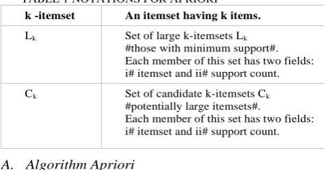
In this section we will revisit Apriori algorithm. Notation We assume that items in each transaction are kept sorted in their lexicographic order. It is straightforward to adapt these algorithms to the case where the database DB is kept normalized and each given database record is a <TID, item> pair, where TID is the identifier of the corresponding transaction. We call the number of items in an itemset its size, and call an itemset of size k a k-itemset. Items within an itemset are kept in lexicographic order. We use the notation c[1].c[2]. . . c[k] to represent a k-itemset c consisting of items c[1], c[2], ... , c[k], where c[1] < c[2] < . . . < c[k]. if c is XY is an m-itemset, we also call Y an m-extension of X. Associated with each itemset is a count field to store the support for this itemset. The count field is initialized to zero when the itemset is first credited summarize in table 1 the notation used in the algorithms.
TABLE 1 NOTATIONS FOR APRIORI
k -itemset An itemset having k items.
Lk Set of large k-itemsets Lk
#those with minimum support#. Each member of this set has two fields: i# itemset and ii# support count.
Ck Set of candidate k-itemsets Ck
#potentially large itemsets#.
Each member of this set has two fields: i# itemset and ii# support count.
A. Algorithm Apriori
Figure 1 gives the Apriori algorithm. The first pass of the algorithm simply counts item occurrences to determine the large 1-itemsets. A subsequent pass, say pass k, consists of two phases. First, the large itemsets Lk-1 found in the (k-1)th pass are used to generate the candidate itemsets Ck, using the apriori gen function described in 2.1.1. Next the database is scanned and the support of candidates in Ck is counted. For fast counting, we need to efficiently determine candidates in Ck that are contained in a given transaction t. See [5] for a discussion of buffer management.
1) L1 = { large 1-itemsets } ; 2) for ( k = 2; Lk-1≠ Φ ; k++ ) do begin
3) Ck = apriori-gen(Lk-1 ); // New candidates 4) forall transactions t Є D do begin
5) Ct = subset(Ck , t); // Candidates contained in t 6) forall candidates c Є Ct do
7) c.count++; 8) end
9) Lk = { c Є Ck | c.count ≥ minsup }
10) end
11) Answer = ∪k Lk ; Figure 1: Algorithm Apriori
B. The apriori-gen function
The apriori-gen function takes as argument Lk-1, the set of all large (k-1)-itemsets. It returns a superset of the set of all large k-itemsets. The function works as follows. 1 First, in the join step, we join Lk-1 with Lk-1 : the logic implemented using sql query form is as follows;
(1) insert into Ck
select p.item[1], p.item[2], ... , p.item[k-1], q.item[k-1]
from Lk-1 p, Lk-1 q
where p.item[1] = q.item[1], ... , p.item[k-2] = q.item[k-2], p.item[k-1] < q.item[k-1];
Next, in the prune step, we delete all itemsets c Є Ck itemsets such that some (k-1)-subset of c is not in Lk-1
(1) forall itemsets c Є Ck do forall (k-1)-subsets s of c do
if ( c not belongs to L[k-1] ) then delete c from Ck ;
III. PROBABILISTIC FREQUENTANDASSOCIATION
RULEMINING
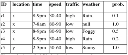
traffic volume) are captured by a red-light camera system, which contains sensors and cameras mounted in road intersections. Each tuple is annotated by a probability that a true violation happens. The probability that a violation occurs is determined by sensor measurement errors, as well as the uncertainty caused by automatic information extraction of the photographs taken by the system [53].
ID location time speed traffic weather prob.
t1 x 8-9pm 30-40 high Rain 0.1
t2 x 7-8am 80-90 low null 1.0
t3 x 8-9pm 80-90 low Foggy 0.5
t4 x 8-9pm 30-40 high Rain 0.2
t5 y 2-3pm 50-60 low Sunny 1.0
Figure 2: A probabilistic database example
To interpret tuple uncertainty, the Possible World Semantics (or PWS in short) is often used [34]. Conceptually, a database is viewed as a set of deterministic instances (called possible worlds), each of which contains a set of zero or more tuples. A possible world for Figure 2 consists of the tuples { t2, t3, t5 }, existing with a probability of (1 - 0.1) x 1.0 x 0.5 x ( 1 - 0.2) x 1.0 = 0.036. Any query evaluation algorithm for probabilistic database has to be correct under PWS. That is, the results produced by the algorithm should be the same as if the query is evaluated on every possible world[34] Although PWS is intuitive and useful, evaluating queries under this notion is costly. This is because a probabilistic database has an exponential number of possible worlds. For example, the table in Figure 1 has 23 = 8 possible worlds. Performing query evaluation or data mining under PWS can thus be technically challenging. In fact, the mining of uncertain or probabilistic data has recently attracted research attention [26]. In [41], efficient clustering algorithms were developed to group uncertain objects that are close to each other. Recently, a Naive Bayes classifier has been developed [49]. The goals of this paper are: (1) propose a definition of frequent patterns and association rules for the tuple uncertainty model; and (2) develop efficient algorithm for mining frequent patterns and association rules.
Association rule Probability
r1: {location=x} ⇒ {time=8-9pm} r2: {location=x} ⇒ {speed=80-90,traffic=low}
0.15 0.49
Figure 3: Sample p-ARs derived from Figure 2
The frequent patterns discovered from probabilistic data are also probabilistic, to reflect the confidence placed on the mining results. Figure 3 shows two probabilistic frequent patterns (or p-FP) extracted from the database in Figure 2. A p-FP is a set of attribute values that occur frequently with sufficiently high probabilities. The pmf of the number of tuples is the support count that contains a pattern
with specific probability. Under PWS, a database is a set of possible worlds, each of which records a (different) support of the same pattern. Hence, the support of a frequent pattern is a pmf. In figure 1, if we consider all possible worlds where { location = x }occurs three times, the pmf of { location = x } with a support of 3 is 0.49. for the p-FP shown. Figure 3 displays their related probabilistic association rules (or p-ARs). Here, rule r2 suggests that with a 0.49 probability, 1) red-light violations occur frequently at location x and 2) when this happens, the involved vehicle is likely driving at a high speed amid low traffic. We will later explain more about the semantics of p-FP and p-AR. A simple way of finding p-FPs is to extract frequent pat- terns from every possible world. This is practically infeasible, since the number of possible worlds is exponentially large.
Prior work. [30] studied approximate frequent patterns on noisy data, while [42] examined association rules on fuzzy sets. The notion of a “vague association rule” was developed in [43]. These solutions were not developed on probabilistic data models. For probabilistic databases, [32, 25] derived patterns based on their expected support counts. [54, 50] found that the use of expected support may render important patterns missing. They discussed the computation of the probability that a pattern is frequent. While [55] handled the mining of single items, our solution can discover patterns with more than one item. The data model used in [50] assumes that for each tuple, each attribute value has a probability of being correct. This is different from the tuple-uncertainty model, which describes the joint probability of attribute values within a tuple. Pmf evaluation method DC algorithm is asymptotically faster than the DP algorithms used in [54, 50], and is thus more scalable for large and dense datasets. To our best knowledge, none of the above works considered the important problem of generating association rules on probabilistic databases.
This section is organized as follows. Section 3.1 introduces the notions of p-FPs and p-ARs. Sections 3.2 present our algorithms for mining p-FPs. Section 3.3 discusses fully solved example using dataset used in paper introduced Pascal algorithm. The CIPFP algorithm is described in section 5 and example is described in section 6
A. Problem Definition
We first review frequent patterns and association rules in Sections 3.1.1. Then, we discuss the uncertain data model in Section 3.1.2. We present the problems of mining p-FPs and p-ARs, in Sections 3.1.3 and 3.1.4.
database of size n and a pattern X, we use sup(X) to denote the support of X, i.e., the number of times that X appears in the database. A pattern X is frequent if:
sup(X) minsup (1)
where minsup ∈ N ∩ [1, n] is the support threshold [27].
Given patterns X and Y (with X∩Y = Ø), if pattern XY is frequent, then X is also frequent (called the anti-monotonicity property). Also, X⇒Y is an association rule if following conditions holds:
supp(XY) ≥ minsup (2)
supp(XY)/supp(X) ≥ minconf (3)
sup(XY) / sup(X), denoted by conf(X⇒Y), is the confidence of X⇒Y, and minconf ∈ R ∩ (0, 1] is the confidence threshold. To verify Equation 3, the values of sup(XY) and sup(X) have to be found first. We remark that a transaction database is essentially a relational table with asymmetric binary attribute values. For example, the existence of item “apple” in a transaction is equivalent to a binary attribute of a tuple with a value of 1. This kind of attributes, assumed in this paper, is also considered by some mining algorithms (e.g., [27, 28]). To handle other attribute types (e.g., continuous and categorical), discretization and binarization techniques can be used to convert them to binary attributes [52].
2) The Possible World Semantics
We assume that each transaction has an existential probability, which specifies the chance that the transaction exists. Figure 4(a) illustrates this database, in which each transaction is a set of items represented by letters. This model has been used to capture uncertainty in many applications, including data streams[33] and geographical services[45].
Now, let P(E) be the probability that an event E occurs and PDB be probabilistic database of size n. Also, let Ti (where i = 1, ..., n ) be the ID of each tuple in PDB. Suppose Ti.S is the set of items contained in Ti, and Ti.p is the existential probability of Ti.
ID SetOfItems Probability/
confidence
T 1 {a, c, e, g, i} 0.6
T 2 {a, c, f, h} 0.5
T 3 {a, d, e, g, j} 0.7
T 4 {b, d, f, h, i} 1.0
Figure 4(a) A probabilistic database
Under PWS, PDB is a set of possible worlds W. Figure 4(b) lists all possible worlds for figure 4(a). Each Wi ε W exists with probability P(Wi). For example P(W2) = T1.p X ( 1 – T2.p) X ( 1 -T3.p) X T4.p or 0.09. The sum of possible world probabilities is one. Also, the number of possible worlds is exponentially large, i.e. |w| = O( 2n). Our goal is to discover patterns and rule using these possible worlds.
W Tuples in W Prob. W Tuples in W Prob.
W1 T4 0.06 W5 T1, T2, T4 0.09
W2 T1, T4 0.09 W6 T1, T3, T4 0.21
W3 T2, T4 0.06 W7 T2, T3, T4 0.14
W4 T3, T4 0.14 W8 T1, T2, T3, T4 0.21
Figure 4(b) Possible World for PDB in Figure 4(a)
B. Probabilistic Frequent Patterns
We first explain the concept of support for probabilistic data. Given a pattern X, we denote its support in each world Wi as supi(X) is obtained by counting the number of times X appears in Wi. Since each Wi exists with a probability, the support of X in PDB, i.e. sup(X), is a random variable. We denote fX(k) that the probability mass function (pmf) of sup(X) can take. Specifically, fX(k) is the probability that sup(X) = k, and fX(k) = 0 for any k ∉ [0,n]. We use an array to store the non-zero values of fX, where fX[k] = P(supp(X) = k). Figure 4(c) depicts the support pmf of {a}. the probability that sup({a}) = 1 is 0.29.
DEFINITION 1. A pattern X is a probabilistic frequent pattern or p-FP in PDB if
P(sup(X) ≥ minsup) ≥ minprob (4)
where minprob є R ∩ (0,1] is the probability threshold.
Problem 1 (p-FP Mining). Given PDB, minsup and minprob, return a set of {X, fX(k), where X is a FP .As we will discuss, the pmfs obtained with p-FPs are essential to generating probabilistic association rules. There are methods to approximating and compressing pmfs (e.g., see [35]). Here we assume that the pmf is exact, but our
solutions can be extended to support these schemes. Next, we present a useful lemma.
Lemma 1 (Anti-monotonicity). If pattern X is a p-FP, then any pattern X' ⊂ X is also a p-FP.
The anti-monotonicity property is true for frequent patterns in exact data [27]. Lemma 1 allows us to stop examining a pattern, if any of its sub-pattern is not a p-FP. A p-FP X is said to be maximal if we cannot find another p-FP Y such that X ⊂ Y . A maximal p-FP can succinctly represent a set of p-FPs when their supports are not concerned. Since the mining of maximal frequent patterns is an important problem [28] for exact data, we also study maximal p-FPs, together with free set, maximal set make a complete system, we study them too,:
Problem 2.1 (Free set p-FP Mining). Given a database PDB, minsup and minprob, return all minimal generators or free sets p-Fps.
Problem 2.2 (Maximal p-FP Mining). Given a database PDB, minsup and minprob, return all maximal p-Fps.
Problem 2.3 (closed p-FP Mining). Given a database PDB, minsup and minprob, return all closed p-FPs.
C. Probabilistic Association Rules
In a probabilistic database, the support counts of patterns are random variables. Let P (X⇒Y) be the probability that X⇒Y is an association rule. By Equations 2 and 3, we have:
P (X⇒Y) = P [sup(XY ) > minsup∧ conf (X⇒Y) ≥ minconf] (5)
Definition 2. X⇒Y is a probabilistic association rule (p-AR in short) if
P (X ⇒ Y ) ≥ minprob (6)
The problem of p-AR mining is defined as follows.
Problem 3 (p-AR Mining). Given minsup, minprob, minconf, and the p-FPs and their support pmfs obtained from Problem 1, derive all p-ARs and their probabilities.
A simple way of solving Problems 1, 2, and 3 is to expand PDB into all possible worlds, compute patterns and rules from each world, and then combine the results. If minsup=2, minconf=0.5, and minprob=0.2, for Figure 4(a), {a}⇒{c} is an association rule only in worlds W5 and W8 (Figure 4(c)), with P ({a}⇒{c}= Pr(W5) + Pr(W 8) = 0.09 + 0.21 = 0.3. Since this is larger than 0.2, {a}⇒{c} is a p-AR. This method is not practical , due to the large number of possible worlds. To tackle Problems 1 and 2, proposed algorithms, namely probabilistic Apriori discussed and solved fully in next section 4.
IV. PROBABILISTIC APRIORI USING PWS FULLY SOLVED CASE
In this section we display the probabilistic Apriori using PWS fully Solved using toy database used in research paper by Bastides et. al. described algorithm Pascal. To solve Problem 1, we discussed the probabilistic-Apriori algorithm, which is an adaptation of the Apriori algorithm [27] for probabilistic databases. Specifically, probabilistic-Apriori uses the bottom-up framework [27]: using PWS.
A. Our Probabilistic Algorithm: ProbabilisticApriori
1. PDB Database making, 2. PWS making using PDB,
3. Define candidate C1 1-itemset equal to Item Collection I. 4. PDB database scan for all c belongs to C1 to calculate support c.support. Store them in a list call it FP.
5. PWS database scan for all c in FP and all c.support where support is equal to “0” to “c.support” to evaluate
fc[k]probability pmf support.
6. Determining Probabilistic Frequent Patterns using minsup and minprob. First compare minsup with c.support. If c.support ≥ minsup than using pmf for pattern c in C1 compare fc[k] ≥ minprob. Collect all c in PFP and assign it to L1 all along with valid frequent probable support and probability. Call it L1.
7.1) L1 = { large 1-itemsets } ; 7.2) for ( k = 2; Lk-1≠ Φ ; k++ ) do begin
7.3) Ck = apriori-gen(Lk-1 ); // New candidates 7.4) forall transactions t Є PDB do begin
7.5) Ct = subset(Ck , t); // Candidates contained in t 7.6) forall candidates c Є Ct do
7.7) c.count++; 7.8) end
7.9) FP = { c Є Ck | c.count ≥ minsup } 7.10) forall fp Є FP
7.11) from k = 0 to fp.support
7.12) W = w Є PWS exactly with size k times k number of transactions
7.13) Ffp[k].prob++;
7.14) end
7.15) PFP = { FP Є FPk | Ffp[k].prob ≥ minprob } 7.15) Lk = PFP
10) end
11) Answer = ∪k Lk ;
Figure 5: Probabilistic Apriori Algorithm
B. The apriori-gen function
The apriori-gen function takes as argument Lk-1, the set of all large (k-1)-itemsets. It returns a superset of the set of all large k-itemsets. The function works as follows. 1 First, in the join step, we join Lk-1 with Lk-1 : the logic is in the form of sql query form is as follows;
(1) Insert into Ck
select p.item[1], p.item[2], ... , p.item[k-1], q.item[k-1] from Lk-1 p, Lk-1 q
where p.item[1] = q.item[1], ... , p.item[k-2] = q.item[k-2], p.item[k-1] < q.item[k-1];
Next, in the prune step, we delete all itemsets c Є Ck itemsets such that some (k-1)-subset of c is not in Lk-1.
(1) forall itemsets c Є Ck do forall (k-1)-subsets s of c do
if ( c not belongs to Lk-1 ) then
C. Solved Example Probabilistic Apriori
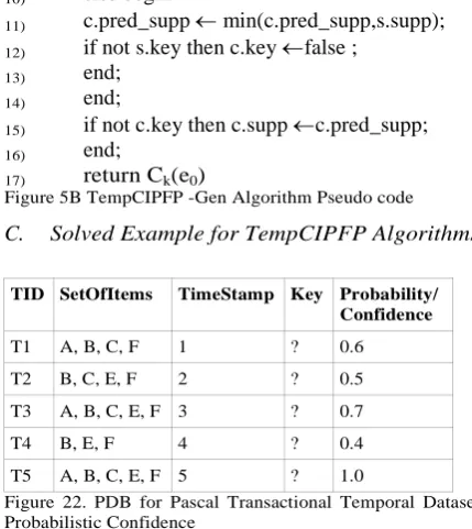
This section discusses the solved example of probabilistic Apriori on toy database. To explain fully general version is solved to full length. The database used is same as used is paper which presented Pascal Algorithm extended to include the transaction level existential probability and time stamp for time at which transaction took place. Figure 6 depicts Pascal Transaction Temporal Dataset with Probabilistic Confidence. For our Probabilistic Apriori algorithm only column TID, SetOfItems, and Probabilistic/Confidence are of importance or relevant.
TID SetOfItems TimeStamp Key Probability/Confidenc e
T1 A, B, C, F 1 ? 0.6
T2 B, C, E, F 2 ? 0.5
T3 A, B, C, E, F 3 ? 0.7
T4 B, E, F 4 ? 0.4
T5 A, B, C, E, F 5 ? 1.0
Figure 6. PDB for Pascal Transactional Temporal Dataset with Probabilistic Confidence
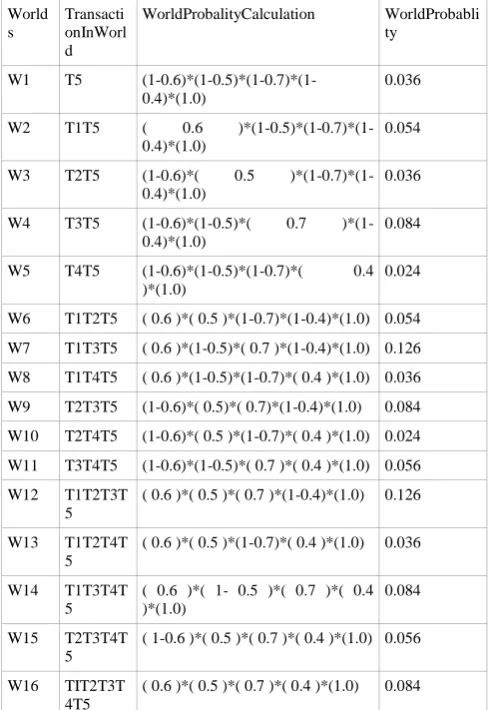
Using concepts of Possible World Semantics in earlier sections, on database presented in Figure 6 we calculated PWS, which is available in Figure 7.
World s
Transacti onInWorl d
WorldProbalityCalculation WorldProbabli ty
W1 T5 (1-0.6)*(1-0.5)*(1-0.7)*(1-0.4)*(1.0)
0.036
W2 T1T5 ( 0.6 )*(1-0.5)*(1-0.7)*(1-0.4)*(1.0)
0.054
W3 T2T5 (1-0.6)*( 0.5 )*(1-0.7)*(1-0.4)*(1.0)
0.036
W4 T3T5 (1-0.6)*(1-0.5)*( 0.7 )*(1-0.4)*(1.0)
0.084
W5 T4T5 (1-0.6)*(1-0.5)*(1-0.7)*( 0.4 )*(1.0)
0.024
W6 T1T2T5 ( 0.6 )*( 0.5 )*(1-0.7)*(1-0.4)*(1.0) 0.054
W7 T1T3T5 ( 0.6 )*(1-0.5)*( 0.7 )*(1-0.4)*(1.0) 0.126
W8 T1T4T5 ( 0.6 )*(1-0.5)*(1-0.7)*( 0.4 )*(1.0) 0.036
W9 T2T3T5 (1-0.6)*( 0.5)*( 0.7)*(1-0.4)*(1.0) 0.084
W10 T2T4T5 (1-0.6)*( 0.5 )*(1-0.7)*( 0.4 )*(1.0) 0.024
W11 T3T4T5 (1-0.6)*(1-0.5)*( 0.7 )*( 0.4 )*(1.0) 0.056
W12 T1T2T3T 5
( 0.6 )*( 0.5 )*( 0.7 )*(1-0.4)*(1.0) 0.126
W13 T1T2T4T 5
( 0.6 )*( 0.5 )*(1-0.7)*( 0.4 )*(1.0) 0.036
W14 T1T3T4T 5
( 0.6 )*( 1- 0.5 )*( 0.7 )*( 0.4 )*(1.0)
0.084
W15 T2T3T4T 5
( 1-0.6 )*( 0.5 )*( 0.7 )*( 0.4 )*(1.0) 0.056
W16 TIT2T3T 4T5
( 0.6 )*( 0.5 )*( 0.7 )*( 0.4 )*(1.0) 0.084
Figure 7. PWS for PDB for Pascal Transactional Temporal Dataset with Probabilistic Confidence
The collection of Items for figure 6 PDB contains 6 individual items, let say I is the set of these items. Hence I = { A, B, C, D, E, F }, For this example minsup is 2/5 that is 40%. As total number of transactions in database i.e. the size of database n is 5. So, the threshold for minsup will be given by (5 * 40 ) /100, i.e 2. So, minsup is 2, let minprob is 0. We are taking minprob 0 to show that algorithm will behave exactly as apriori behave when no probabilistic transaction is considered. This is equivalent to treating all transactions having certainty or probability of 1 to occur.
All the elements which belongs to collection I will become the candidate pattern, as the individual items themselves are used as patterns we call them 1-itemset. The collection of candidate 1-itemset denoted as C1 is as follows: C1= { {A}, {B},{C},{D},{E},{F}} for each element c belongs to C1 we calculate its support in database PDB Figure 6. For all itemset the PDB database scan output is as follows:
Pattern/1-itemset Support in PDB
{A} 3
{B} 4
{C} 4
{D} 1
{E} 4
{F} 5
Figure 8. C1 and its Support Count
In the figure 8 if we compare support of respective patterns we found that pattern {D} has a support 1 which is less than the minimum support. sup({D}) < minsup. So the set of frequent 1-itemset FP1 will contain all 1-itemset from figure 8 but not {D}.This set of frequent 1-itemset FP1 is as follows;
Pattern/1-itemset Support in PDB
{A} 3
{B} 4
{C} 4
{E} 4
{F} 5
Figure 9 FP1 set of frequent 1-itemset
universe, means any Wi that contain exactly one time any of the {A}.Ti, i.e., Wi exactly contain either one of T1, or T2, or T2 but not T1T2, T1T3 or T2T3 or T1T2T3 together, all their probabilities will be summed up. For {A}.support is 1, PWS is W1W3W5W10 with probability 0.036, 0.036, 0.024, 0.024 summed up to 0.12, this 0.12 is existential probability of pattern {A} when its support is 1. Like wise we calculate for all fp belongs to FP1. The following figure 10 summaries C1 PFP1 patterns with their support pmf values. “-” represents not required status.
Support\Pattern {A} {B} {C} {D} {E} {F}
0 0 0 0 0.4 0 0
1 0.12 0.09 0.06 0.6 0.09 0.036
2 0.46 0.36 0.29 - 0.36 0.198
3 0.42 0.41 0.44 - 0.41 0.380
4 - 0.14 0.21 - 0.14 0.246
5 - - - 0.140
Figure 10. C1 candidate PFP1 patterns with their support pmf values If we compare all 1-itemset support pmf values against minprob we will get PFP 1-itemset. For minprob “0” we will have entire Figure 10 as probabilistic frequent PFP1. So, now using all patterns in PFP1 we will continue and assign this collection to L1 and call apriori_gen on all probabilistically frequent 1-itemset patterns in L1 to generate candidate 2-itemset C2. Using PDB database scan we count their support.
Pattern/2-itemset Support in PDB
{AB} 2
{AC} 3
{AE} 2
{AF} 3
{BC} 3
{BE} 4
{BF} 4
{CE} 3
{CF} 4
{EF} 4
Figure 11. C2 and its Support Count
All pattern in Figure 11 are frequent. So, frequent 2-itemset will be as following in figure 12.
Pattern/2-itemset Support in PDB
{AB} 2
{AC} 3
{AE} 2
{AF} 3
{BC} 3
{BE} 4
{BF} 4
{CE} 3
{CF} 4
{EF} 4
Figure 12. FP2 and its Support Count
The candidate for PFP will be as following in figure 13.
Pattern> SupportV
{AB} {AC} {AE} {AF} {BC} {BE} {BF} {CE} {CF} {EF}
0 0 0 0 0 0 0 0 0 0 0
1 0.3 0.12 0.3 0.12 0.15 0.09 0.09 0.15 0.06 0.09 2 0.7 0.46 0.7 0.46 0.50 0.36 0.36 0.50 0.29 0.36 3 - 0.42 - 0.42 0.35 0.41 0.41 0.35 0.44 0.41 4 - - - 0.14 0.14 - 0.21 0.14
5 - - -
-Figure 13. C2 candidate PFP2 patterns with their support pmf values.
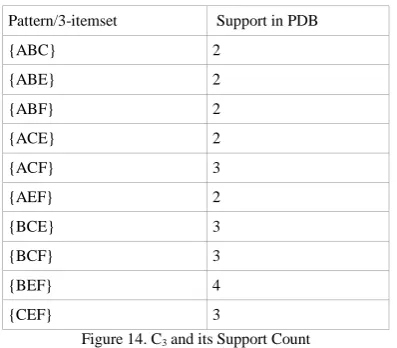
All candidate PFP2 are probabilistic frequent hence we treat patterns in figure 13 as PFP and finally as L2. These 2-itemset probabilistically frequent patterns in L2 will be used to generate candidate 3-itemset patterns.
Pattern/3-itemset Support in PDB
{ABC} 2
{ABE} 2
{ABF} 2
{ACE} 2
{ACF} 3
{AEF} 2
{BCE} 3
{BCF} 3
{BEF} 4
{CEF} 3
Figure 14. C3 and its Support Count
All pattern in Figure 14 are frequent. So, frequent 3-itemset will be as following in figure 15.
Pattern/3-itemset Support in PDB
{ABC} 2
{ABE} 2
{ABF} 2
{ACE} 2
{ACF} 3
{AEF} 2
{BCE} 3
{BCF} 3
{BEF} 4
{CEF} 3
Figure 15. FP3 and its Support Count
The candidate for PFP will be as following in figure 16.
Pattern Support
{ABC} {ABE} {ABF} {ACE} {ACF} {AEF} {BCE} {BCF} {BEF} {CEF}
0 0 0 0 0 0 0 0 0 0 0
1 0.264 0.264 0.264 0.264 0.264 0.264 0.15 0.15 0.09 0.15 2 0.736 0.736 0.736 0.736 0.736 0.736 0.50 0.50 0.36 0.50
3 - - - 0.35 0.35 0.41 0.35
4 - - - 0.14
-Figure 16. C3 candidate PFP3 patterns with their support pmf values.
All candidate PFP3 are probabilistic frequent hence we treat patterns in figure 16 as PFP and finally as L3. These 3-itemset probabilistically frequent patterns in L3 will be used to generate candidate 4-itemset patterns, which are as follows;
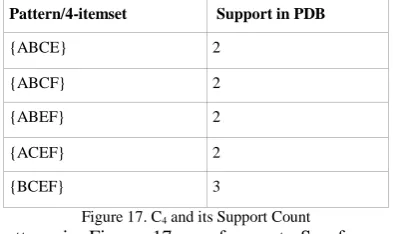
Pattern/4-itemset Support in PDB
{ABCE} 2
{ABCF} 2
{ABEF} 2
{ACEF} 2
{BCEF} 3
Figure 17. C4 and its Support Count
All pattern in Figure 17 are frequent. So, frequent 3-itemset will be as following in figure 18.
Pattern/4-itemset Support in PDB
{ABCE} 2
{ABCF} 2
{ABEF} 2
{ACEF} 2
{BCEF} 3
Figure 18. FP4 and its Support Count
The candidate for PFP will be as following in figure 19.
Support\Patter n
{ABCE} {ABCF} {ABEF} {ACEF }
{BCEF}
0 0 0 0 0
1 0.264 0.264 0.264 0.264 0.15
2 0.736 0.736 0.736 0.736 0.50
3 - - - - 0.35
4 - - - -
-5 - - - -
-Figure 19. C4 candidate PFP4 patterns with their support pmf values.
All candidate PFP4 are probabilistic frequent hence we treat patterns in figure 19 as PFP and finally as L4. These 4-itemset probabilistically frequent patterns in L4 will be used to generate candidate 5-itemset patterns, which are as follows;
Pattern/4-itemset Support in PDB
{ABCE} 2
Figure 20. C5 and its Support Count
All pattern in Figure 20 are frequent. So, frequent 3-itemset will be as following in figure 21.
Pattern/5-itemset Support in PDB
{ABCEF} 2
Figure 21. FP5 and its Support Count
The candidate for PFP will be as following in figure 22. Support\Pattern {ABCEF}
0 0
1 0.264
2 0.736
3 -
4 -
5 -
Figure 22. C5 candidate PFP5 patterns with their support pmf values.
All candidate PFP5 are probabilistic frequent hence we treat patterns in figure 22 as PFP and finally as L5. These 5-itemset probabilistically frequent patterns in L5 will be used to generate candidate 6-itemset patterns. But no more new candidate 6-itemset are possible so algorithm execution stops here.
V. TEMPORALCIPFPALGORITHM In this section we will discuss TempCIPFP algorithm. This algorithm is an extension of CTPFP Algorithm. Extension exploits the concepts of key patterns and calendar schema patterns in combination on probabilistic database given in figure 6. In the section 5.1.1 first we explain basic concepts of counting inference, in section 5.1.2 discuss calender schema pattern and mining time stamped databases problem, and than in section 5.2 we will describe the pseudo-code for our TempCIPFP algorithm, in next section 5.3 we will illustrate the algorithm's functioning with the help of a toy dataset fully solved example.
A. Basic Concepts of Temporal Counting Inference 1) Key patterns and pattern Counting Inference
Definition 5.1. Let P be a finite set of items, O a finite set of objects (e.g., transaction ids) and R ⊆O x P a binary relation (where (o, p) R may be read as “item p is included in transaction o”). The triple D=(O, P, R) is called dataset Each subset p of P is called a pattern. We say that a Pattern P is included in an object o O if (o,p) R for all p P. Let f be the function which assign to each pattern p ⊆P the set of all objects which include this pattern : f(P) = { o O | o includes P }. The support of a pattern P is given by supp(P) = card (f (P))/card (O). For a given threshold minsup [0,1], a pattern P is called frequent pattern if supp(P) ≥ minsup.
Definition 5.2. A K-pattern p is a subset of P with card (P) = K. A candidate K-pattern where all its proper sub-patterns are frequent.
Definition 5.4. A pattern P is a key pattern if P min [P]. A candidate key pattern is a pattern where all its proper sub patterns are frequent key patterns.
Theorem 5A (i ) if Q is a key pattern and P Q ,then P is also a key pattern.
(ii) if P is not a key pattern and, P Q then Q is not a key pattern either.
Theorem 5B. Let P be a pattern.(i) Let p P then P [P \{p}] if and only if supp(P)= supp(P\ {p})
(ii) P is a key pattern if and only if supp(P) ≠ min p P (supp(P\{p}))
Theorem 5C. Let P is a non key pattern then supp(P)= min p P (supp(P\{p}))
2) Simple Calendar-based Pattern
An interesting extension to association rules is to include a temporal dimension. For example, if we look at a database of transactions in a supermarket, we may find that sweets and crackers are seldom sold together. However, if we only look at the transactions in the week before diwali, we may discover that most transactions contain sweets and crackers, i.e., the association rule “sweets->crackers” has a high support and a high confidence in the transactions that happen in the week before diwali. The above suggests that we may discover different association rules if different time intervals are considered. Informally, we refer to the association rules along with their temporal intervals as temporal association rules. In this paper, we use calendar schema[57] as frameworks to discover temporal association rules. A hierarchy of calendar units determines a calendar schema. For example, a calendar schema can be (year, month, day). A calendar schema defines a set of simple calendar-based patterns (or calendar patterns for short). For example, given the above calendar schema, we will have calendar patterns such as every day of January of 1999 and every 16th day of January of every year. Basically, a calendar pattern is formed for a calendar schema by fixing some of the calendar units to specific numbers while leaving other units “free” (so it’s read as “every”). It is clear that each calendar pattern defines a set of time intervals. We assume that the transactions are time stamped so we can decide if a transaction happens during a specific time interval. Given a set of transactions and a calendar schema, our first interest is to discover all pairs of association rule and calendar pattern such that for each pair (r; e), the association rule r satisfies the minimum support and confidence constraint among all the transactions that happen during each time interval given by the calendar pattern e. For example, we may have an association rule sweets-> crackers along with the calendar pattern every day in every November. We call the resulting rules temporal association rules w.r.t. Precise match[57]. In some applications, the above temporal association rules may be too restrictive. Instead, we may require that the association rule hold during “enough” number of intervals given by the corresponding calendar pattern. For example, the association rule sweets-> crackers may not hold on every day of every November, but holds on more than 80% of November days. We call such rules temporal association rules w.r.t. Fuzzy match[57]. When temporal information is applied in terms of date, month, year & week, form the term Calendar schema. it is introduced in temporal data
mining. A calendar schema is a relational Schema R =( Gn : Dn,Gn-1 : Dn-1,……, G1 : D1) together with a valid constraint[57]. Each attribute Gi is a granularity name like year, month and week. Each domain Di is a finite subset of the Positive integers. A calendar schema (year: {2007,2006….}, month: 1,2,3,4…12}, day{1,2,3…..31}) with the constraints is valid if that evaluates(yy,mm,dd) to true only If the combination gives a valid date while <1996,2,31> is not. In calendar pattern, the branch e cover e’ in the same Calendar schema if the time interval e’ is the subset of e and they all follow the same pattern. If a calendar patterns <dn,dn-1,…..d1> covers another pattern <d’n,d’n-1,…..d’1> if and only if for each I, 1<= I <= n or di = d’I .Now our task is to mine frequent pattern over arbitrary time interval in terms of calendar pattern schema.
3) Temporal Association rule
Definition 1: The frequency of itemset over a time period T is the number of transactions in which it occurs divided by total number of transaction over a time period. In the same way, confidence of an item with another item is the transaction of both items over the period divided by first item of that period. Support (A)= Frequency of occurrence of A in specified time interval / total no of tuples in Specified time interval.
Confidence (A=>B [Ts, Te]) = Support count (A B) over interval /occurrence of A in interval. Ts indicates the valid start time & Te indicate valid time according to temporal data .
B. Our Temporal TempCIPFP Algorithm
Mining temporal association rules in probabilistic databases can be decomposed into two steps: (1) finding all Frequent item sets for all star calendar patterns on the given calendar schema against the given thresholds for minsup and minprob, and (2) generating Temporal association rules using the probabilistic frequent item sets and their calendar pattern and minconf threshold. The first step is the crux of the discovery of temporal association rule; in the following, we will focus on this problem. The pseudo-code is given in algorithm TempCIPFP. The proposed algorithm is as follows,
Algorithm 1 CIPFP:
[1] .supp 1 ; .Key true; [2] P0 {}
[3] For all basic time interval e0 do begin [4] P1 (e0) { frequent 1-pattern in T[e0] } [5] For all p P1(e0) do begin
[6] p.pred_supp 1 ;p.Key (p.supp 1) ; [7] end;
for all star pattern e that cover e0 do [8] update P1 (e) using P(e0) ;
[9] FP1 = { c Є P1 | c.count ≥ minsup } [10] forall fp Є FP1
[11] from k = 0 to fp.support
[12] W = w Є PWS exactly with size k times k number of transactions
[15] PFP = { FP Є FP1 | Ffp[k].prob ≥ minprob } [16] P1 = PFP
[17] end [18]end
[19]for (k=2 ; a star calendar pattern e such that Pk-1 (e) ,K++) do begin
[20]for all basic time interval e0 do begin // Phase I: generate candidates
[21]Ck(e0) TempCIPFP-Gen(Pk-1(e0)) // Phase II: Scan the transactions [22]For all transaction T T[e0] do [23]If C Ck(e0) | C.key then [24]For all o D do begin
[25] C0 Subset (Ck(e0 ) ,O, T) // C.count ++ if // c Ck (e0) is contained in T
[26]for all C C0 | C.Key do [27]c.supp ++
[28]end ;
[29]for all c Ck(e0)do
[30]if c.supp minsup then begin
[31]if c.key and c.supp = c.pred_supp then [32]c.key False ;
[33]Pk (e0) Pk (e0) {c } [34]End
// Phase III : update for star calendar patterns [35]for all star pattern e that cover e0 do [36]update Pk (e) using Pk (e0)
[37]end
[38]FP = { c Є Pk | c.count ≥ minsup } [39] forall fp Є FP
[40] from k = 0 to fp.support
[41] W = w Є PWS exactly with size k times k number of transactions
[42] Ffp[k].prob++; [43] end
[44] PFP = { FP Є FPk | Ffp[k].prob ≥ minprob } [45] Pk = PFP
[46] end
[47]Output <Pk (e), e> for all star calendar pattern e [48]End
Figure 5A TempCIPFP Algorithm Pseudo code
Algorithm 2 TempCIPFP-Gen
Input : Pk-1(e0) , the set of frequent (K-1) patterns p with their support p.supp and the p.key flag.
Output: Ck(e0),the set of candidate k patterns c each with the flag c.key,the value c.pred_supp,and the support c.supp if c is not a key pattern
1) insert into Ck(e0) select p.item1 ,p.item2 ,……p.itemk-1,q.itemk-1
2) from Pk-1 p, Pk-1 q
3) Where p.item1 = q.item1, ……. p.itemk-2 = q.item k-2, p.itemk-1 < q.itemk-1;
4)
5) for all c Ck(e0) do begin 6) c.key true ; c.pred_supp + ; 7) for all (k-1) subsets s of c do begin 8) if s Pk-1(e0) then
9) delete c from Ck(e0) ; 10) else begin
11) c.pred_supp min(c.pred_supp,s.supp); 12) if not s.key then c.key false ;
13) end; 14) end;
15) if not c.key then c.supp c.pred_supp;
16) end;
17) return Ck(e0)
Figure 5B TempCIPFP -Gen Algorithm Pseudo code
C. Solved Example for TempCIPFP Algorithms
TID SetOfItems TimeStamp Key Probability/
Confidence
T1 A, B, C, F 1 ? 0.6
T2 B, C, E, F 2 ? 0.5
T3 A, B, C, E, F 3 ? 0.7
T4 B, E, F 4 ? 0.4
T5 A, B, C, E, F 5 ? 1.0
Figure 22. PDB for Pascal Transactional Temporal Dataset with Probabilistic Confidence
Using concepts of Possible World Semantics in earlier sections, on database presented in Figure 6 we calculated PWS, which is available in Figure 7 again displayed here in figure 23.
Possib leWor ldSem antic
Transaction InWorld
WorldProbalityCalculation World
Probabil ity
W1 T5
(1-0.6)*(1-0.5)*(1-0.7)*(1-0.4)*(1.0)
0.036
W2 T1T5 ( 0.6
)*(1-0.5)*(1-0.7)*(1-0.4)*(1.0)
0.054
W3 T2T5 (1-0.6)*( 0.5
)*(1-0.7)*(1-0.4)*(1.0)
0.036
W4 T3T5 (1-0.6)*(1-0.5)*( 0.7
)*(1-0.4)*(1.0)
0.084
W5 T4T5 (1-0.6)*(1-0.5)*(1-0.7)*( 0.4
)*(1.0)
0.024
W6 T1T2T5 ( 0.6 )*( 0.5 )*(1-0.7)*(1-0.4)*(1.0) 0.054
W7 T1T3T5 ( 0.6 )*(1-0.5)*( 0.7 )*(1-0.4)*(1.0) 0.126
W8 T1T4T5 ( 0.6 )*(1-0.5)*(1-0.7)*( 0.4 )*(1.0) 0.036
W9 T2T3T5 (1-0.6)*( 0.5)*( 0.7)*(1-0.4)*(1.0) 0.084
W10 T2T4T5 (1-0.6)*( 0.5 )*(1-0.7)*( 0.4 )*(1.0) 0.024
W11 T3T4T5 (1-0.6)*(1-0.5)*( 0.7 )*( 0.4 )*(1.0) 0.056
W12 T1T2T3T5 ( 0.6 )*( 0.5 )*( 0.7 )*(1-0.4)*(1.0) 0.126
W13 T1T2T4T5 ( 0.6 )*( 0.5 )*(1-0.7)*( 0.4 )*(1.0) 0.036
W14 T1T3T4T5 ( 0.6 )*( 1- 0.5 )*( 0.7 )*( 0.4 )*(1.0)
0.084
W15 T2T3T4T5 ( 1-0.6 )*( 0.5 )*( 0.7 )*( 0.4 )*(1.0) 0.056
W16 TIT2T3T4T5 ( 0.6 )*( 0.5 )*( 0.7 )*( 0.4 )*(1.0) 0.084
Figure 23. PWS for PDB for Pascal Transactional Temporal Dataset with Probabilistic Confidence
= { A, B, C, D, E, F }, For this example minsup is 2/5 that is 40%. As total number of transactions in database i.e. the size of database n is 5. So, the threshold for minsup will be given by (5 * 40 ) /100, i.e 2. So, minsup is 2, let minprob is 0. We are taking minprob 0 to show that algorithm will behave exactly as apriori behave when no probabilistic transaction is considered. This is equivalent to treating all transactions having certainty or probability of 1 to occur.\
TABLE 5.1 NOTATION USED in TempCIPFP
K Is the counter which indicates the current iteration. In the Kth iteration all frequent K-patterns and all key patterns among them are determined.
Pk
Contains after the Kth iteration all frequent k patterns P together with their support P.supp, and a boolean variable P.key indicating if P is a (candidate) key pattern
Ck
Stores the candidate k patterns together with their support (if Known), the Boolean variable P.key and a counter P.pred_supp which stores the minimum of the supports of all (k-1) sub patterns of P
All the elements which belongs to collection I will become the candidate pattern, as the individual items themselves are used as patterns we call them 1-itemset. The collection of candidate 1-itemset
denoted as C1 is as follows:
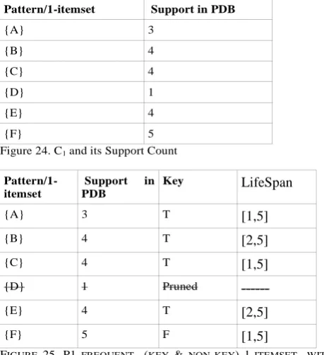
C1={{A},{B},{C},{D},{E},{F}}for each element c belongs to C1 we calculate its support in database PDB Figure 6. The algorithm performs first one database pass to count the support of the 1-itemset pattern (key and non-key both). The candidate pattern{D} is pruned because it is infrequent. Also {F} is marked as non-key because it has the same support as empty set: Now candidate C1 and frequent set of 1-itemset P1 are see figure 24, and figure 25. For all itemset the PDB database scan output is as follows:
Pattern/1-itemset Support in PDB
{A} 3
{B} 4
{C} 4
{D} 1
{E} 4
{F} 5
Figure 24. C1 and its Support Count
Pattern/1-itemset
Support in
PDB
Key LifeSpan
{A} 3 T [1,5]
{B} 4 T [2,5]
{C} 4 T [1,5]
{D} 1 Pruned ---
{E} 4 T [2,5]
{F} 5 F [1,5]
FIGURE 25. P1 FREQUENT (KEY & NON-KEY) 1-ITEMSET WITH SUPPORT
In the figure 25 if we compare support of respective patterns we found that pattern {D} has a support 1 which is less than the minimum support. sup({D}) < minsup. So the set of frequent 1-itemset FP1 will contain all 1-itemset from figure 8 but not {D}.This set of frequent 1-itemset P1 is stored in FP1 is as is given in figure 26.
Pattern/1-itemset Support in PDB Key LifeSpan
{A} 3/5 T [1,5]
{B} 4/5 T [2,5]
{C} 4/5 T [1,5]
{E} 4/5 T [2,5]
{F} 1 F [1,5]
Figure 26 FP1
Now we use patterns in FP1 one by one to calculate their existential probability. For this we first scan PDB and found the TIDs in which pattern is present. For combination of length equal to in range for support from 0 to c.support we start scan of PWS rows and sum up the provabilities of Wi in which exactly the number of transaction present, here the number of transaction which occurred in Wi is determined for every support from 0 to c.support. For example we want to determine existential probability of frequent 1-itemset {A} to determine probabilistic frequent pattern {A} is or not. First, we scan PDB and found that T1, T3, T5 contains {A}. {A}.support is 3. So for transaction combination length of 0, 1, 2, and 3, for example example length 1 means any Wi that contain exactly one time any of the {A}.Ti, i.e., Wi exactly contain either one of T1, or T2, or T2 but not T1T2, T1T3 or T2T3 or T1T2T3 together, all their probabilities will be summed up. For {A}.support is 1, PWS is W1W3W5W10 with probability 0.036, 0.036, 0.024, 0.024 summed up to 0.12, this 0.12 is existential probability of pattern {A} when its support is 1. Like wise we calculate for all fp belongs to FP1. The following figure 10 summaries C1 PFP1 patterns with their support pmf values. “-” represents not required status.
Pattern> SupportV
{A} {B} {C} {D} {E} {F}
0 0 0 0 0.4 0 0
1 0.12 0.09 0.06 0.6 0.09 0.036 2 0.46 0.36 0.29 - 0.36 0.198 3 0.42 0.41 0.44 - 0.41 0.380 4 - 0.14 0.21 - 0.14 0.246
5 - - - 0.140
Figure 27. C1 candidate PFP 1-itemset patterns with their support pmf values
support. At the next iteration, all candidate 2-itemset patterns are created and stored in C2, key and non-key elements are categorized and probabilistic support pmf is evaluated. at the same time the support of pattern containing infrequent pattern {F} as sub-pattern is computed. Then a database pass is performed to determine the support of the remaining six candidate patterns. Hence P2 achieved: Now C2 is see figure 28,
Pattern/2 -itemset
pred_su pp
Key supp LifeSpan
{AB} 3/5 T ? [2,5]
{AC} 3/5 T ? [1,5]
{AE} 4/5 T ? [2,5]
{AF} 3/5 F 3/5 [1,5]
{BC} 4/5 T ? [2,5]
{BE} 4/5 T ? [2,5]
{BF} 4/5 F ? [2,5]
{CE} 4/5 T ? [2,5]
{CF} 4/5 F ? [1,5]
{EF} 4/5 F ? [2,5]
Figure 28. C2 and its Support Count
From this we have Now P2 is see Figure 29.
Pattern/ 2-itemset
supp Key LifeSpan
{AB} 2/5 T [2,5]
{AC} 3/5 F [1,5]
{AE} 2/5 T [2,5]
{AF} 3/5 F [1,5]
{BC} 3/5 T [2,5]
{BE} 4/5 F [2,5]
{BF} 4/5 F [2,5]
{CE} 3/5 T [2,5]
{CF} 4/5 F [1,5]
{EF} 4/5 F [2,5]
Figure 29 P2 frequent (key & non-key) 2-itemset with support All pattern in Figure 29 are frequent. So, frequent 2-itemset will be as following in figure 30.
Pattern/2-itemset
Support in
PDB LifeSpan
{AB} 2 [2,5]
{AC} 3 [1,5]
{AE} 2 [2,5]
{AF} 3 [1,5]
{BC} 3 [2,5]
{BE} 4 [2,5]
{BF} 4 [2,5]
{CE} 3 [2,5]
{CF} 4 [1,5]
{EF} 4 [2,5]
Figure 30. FP2 and its Support Count
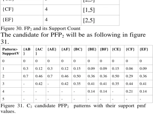
The candidate for PFP2 will be as following in figure 31.
Pattern> SupportV
{AB }
{AC }
{AE} {AF} {BC} {BE} {BF} {CE} {CF} {EF}
0 0 0 0 0 0 0 0 0 0 0
1 0.3 0.12 0.3 0.12 0.15 0.09 0.09 0.15 0.06 0.09 2 0.7 0.46 0.7 0.46 0.50 0.36 0.36 0.50 0.29 0.36 3 - 0.42 - 0.42 0.35 0.41 0.41 0.35 0.44 0.41 4 - - - 0.14 0.14 - 0.21 0.14
5 - - -
-Figure 31. C2 candidate PFP2 patterns with their support pmf values.
All candidate-PFP2 are probabilistic frequent hence we treat all patterns in figure 31 as PFP2 and finally update as P2. These 2-itemset probabilistically frequent patterns in P2 will be used to generate candidate 3-itemset patterns. Repeating again we have Now C3.
Pattern/3 -itemset
pred_su pp
Key supp LifeSpan
{ABC} 2/5 F 2/5 [2,5]
{ABE} 2/5 F 2/5 [2,5]
{ABF} 2/5 F 2/5 [2,5]
{ACE} 2/5 F 2/5 [2,5]
{ACF} 3/5 F 3/5 [1,5]
{AEF} 2/5 F 2/5 [2,5]
{BCE} 3/5 F 3/5 [2,5]
{BCF} 3/5 F 3/5 [2,5]
{BEF} 4/5 F 4/5 [2,5]
{CEF} 3/5 F 3/5 [2,5]
Figure 32. C3 and its Support Count,
All pattern in Figure 32 are frequent. So, frequent 3-itemset will be as following in figure 33.
Pattern/3-itemset
Support in
PDB
LifeSpan
{ABC} 2 [2,5]
{ABE} 2 [2,5]
{ABF} 2 [2,5]
{ACE} 2 [2,5]
{ACF} 3 [1,5]
{AEF} 2 [2,5]
{BCE} 3 [2,5]
{BCF} 3 [2,5]
{BEF} 4 [2,5]
{CEF} 3 [2,5]
The candidate for PFP will be as following in figure 33. As all patterns are non-key in candidyate-PFP3. From now onwards no database scan is required at all to count support. We compute support of higher level pattern using their already determined support of sub patterns. Minimum of support of sub-patterns is used as the support of higher level pattern. But support pmf will be calculated from PDB and PWS scan.
Patte rn> Supp ortV
{AB C}
{AB E}
{A BF }
{AC E}
{AC F}
{AEF }
{B CE }
{BCF }
{BE F}
{CEF}
0 0 0 0 0 0 0 0 0 0 0
1 0.264 0.264 0.26 4
0.264 0.264 0.264 0.15 0.15 0.09 0.15
2 0.736 0.736 0.73 6
0.736 0.736 0.736 0.50 0.50 0.36 0.50
3 - - - 0.35 0.35 0.41 0.35
4 - - - 0.14
-5 - - -
-Figure 34. C3 candidate PFP3 patterns with their support pmf values.
As all candidate-PFP3 are probabilistic frequent hence we treat patterns in figure 34 as PFP3 and finally update P3 by PFP3. These 3-itemset probabilistically frequent patterns in P3 will be used to generate candidate 4-itemset patterns, which are as follows see figure 35. So now in 4th and 5th iteration no database scan is required as we have no key candidate to calculate support in database.
Pattern/4 -itemset
pred_su pp
Key supp LifeSpan
{ABCE} 2/5 F 2/5 [2,5]
{ABCF} 2/5 F 2/5 [2,5]
{ABEF} 2/5 F 2/5 [2,5]
{ACEF} 2/5 F 2/5 [2,5]
{BCEF} 3/5 F 3/5 [2,5]
Figure 35. C4 candidate (key & non-key) 4-itemset with support
All pattern in Figure 35 are frequent. So, frequent 3-itemset will be as following in figure 36.
Pattern/4-itemset
supp Key LifeSpan
{ABCE} 2/5 F [2,5]
{ABCF} 2/5 F [2,5]
{ABEF} 2/5 F [2,5]
{ACEF} 2/5 F [2,5]
{BCEF} 3/5 F [2,5]
Figure 36. FP4 frequent (key & non-key) 4-itemset with support
The candidate for PFP will be as following in figure 37.
Pattern> SupportV
{ABCE }
{ABCF} {ABEF} {ACEF }
{BC EF}
0 0 0 0 0
1 0.264 0.264 0.264 0.264 0.15
2 0.736 0.736 0.736 0.736 0.50
3 - - - - 0.35
4 - - - -
-5 - - - -
-Figure 37. C4 candidate PFP4 patterns with their support pmf values
All candidate PFP4 are probabilistic frequent hence we treat patterns in figure 37 as probabilistically frequent patterns and finally update P4 by PFP4. These 4-itemset probabilistically frequent patterns in P4 will be used to generate candidate 5-itemset patterns, which are as follows;
Pattern/5-itemset
pred_supp Key supp LifeSpan
{ABCEF} 2/5 F 2/5 [2,5]
Figure 38. C5 candidate (key & non-key) 5-itemset with support All pattern in Figure 38 are frequent. So, frequent 5-itemset will be as following in figure 39.
Pattern/5-itemset
Key supp LifeSpan
{ABCEF} F 2/5 [2,5]
Figure 39. FP5 frequent (key & non-key) 5-itemset with support The candidate for PFP will be as following in figure 40.
Support\Pattern {ABCEF}
0 0
1 0.264
2 0.736
3 -
4 -
5 -
Figure 40. C5 candidate PFP5 patterns with their support pmf values
All candidate-PFP5 are having all kth support smf probability greater than minprob hence we treat all of the patterns in figure 40 as probabilistically frequent patterns set PFP5 and finally update P5 by PFP5. These 5-itemset probabilistically frequent patterns in P5 will be used to generate candidate 6-itemset patterns. But no more new candidate 6-iteset are possible so algorithm execution stops here.
VI. CONCLUSION
to encompass this truth of process we studied and suggested a mining procedure that can be used to answer queries which or otherwise only possible to answer on certain data using data mining techniques. To best of our knowledge the steps we carried out are not discuss to this much extent in any paper. Algorithm finally converged with 32 probabilistic frequent patterns were generated when we took the probability of transactions equal to one, i.e. minimum threshold is considered as 0. Many variations in implementation of the algorithm are possible. Also how to select suitable minprob threshold is, depending on this algorithm can be modified. In future we will implement the algorithm with possible alternate implementation as well as mechanism to support selection of minimum support threshold, and selection of minimum probability threshold. The number of DB scan in case of Apriori and probabilistic Apriori are 5, and pattern to be cross checked where 32. But in case of CIPFP algorithm only two database scan are required and only 12 patterns are required to be checked for support in database. Hence CIPFP needs two database passes in which the algorithm counted the support of 6+6=12 patterns. Apriori and Probabilistic Apriori would have needed five database passes for counting supports of 6+6+10+10+5+1=32 patterns for the same dataset.
REFERENCES
[1] R. Agrawal, C. Faloutsos, and A. Swami. Efcient similarity search in sequence databases. In Proc. of the Fourth International Conference on Foundations of Data Organization and Algorithms, Chicago, October 1993.
[2] R. Agrawal, S. Ghosh, T. Imielinski, B. Iyer, and A. Swami. An interval classi er for database mining applications. In Proc. of the VLDB Conference, pages 560{573, Vancouver, British Columbia, Canada, 1992.
[3] R. Agrawal, T. Imielinski, and A. Swami. Database mining: A performance perspective. IEEE Transactions on Knowledge and Data En- gineering, 5(6):914{925, December 1993. Special Issue on Learning and Discovery in Knowledge- Based Databases. [4] R. Agrawal, T. Imielinski, and A. Swami. Mining association rules
between sets of items in large databases. In Proc. of the ACM SIGMOD Con- ference on Management of Data, Washington, D.C., May 1993.
[5] R. Agrawal and R. Srikant. Fast algorithms for mining association rules in large databases. Re- search Report RJ 9839, IBM Almaden Research Center, San Jose, California, June 1994.
[6] D. S. Associates. The new direct marketing. Business One Irwin, Illinois, 1990.
[7] R. Brachman et al. Integrated support for data archeology. In AAAI-93 Workshop on Knowledge Discovery in Databases, July 1993.
[8] L. Breiman, J. H. Friedman, R. A. Olshen, and C. J. Stone. Classi cation and Regression Trees. Wadsworth, Belmont, 1984.
[9] P. Cheeseman et al. Autoclass: A bayesian classi cation system. In 5th Int'l Conf. on Machine Learning. Morgan Kaufman, June 1988. [10] D. H. Fisher. Knowledge acquisition via incremental conceptual
clustering. Machine Learning, 2(2), 1987.
[11] J. Han, Y. Cai, and N. Cercone. Knowledge discovery in databases: An attribute oriented approach. In Proc. of the VLDB Conference, pages 547{559, Vancouver, British Columbia, Canada, 1992. [12] M. Holsheimer and A. Siebes. Data mining: The search for
knowledge in databases. Technical Report CS-R9406, CWI, Netherlands, 1994.
[13] M. Houtsma and A. Swami. Set-oriented mining of association rules. Research Report RJ 9567, IBM Almaden Research Center, San Jose, Cali- fornia, October 1993.
[14] R. Krishnamurthy and T. Imielinski. Practi- tioner problems in need of database research: Re- search directions in knowledge discovery. SIG- MOD RECORD, 20(3):76{78, September 1991.
[15] P. Langley, H. Simon, G. Bradshaw, andJ. Zytkow. Scienti c Discovery: Computational Explorations of the Creative Process. MIT Press, 1987.
[16] H. Mannila and K.-J. Raiha. Dependency inference. In Proc. of the VLDB Conference, pages 155{158, Brighton, England, 1987. [17] H. Mannila, H. Toivonen, and A. I. Verkamo. E cient algorithms
for discovering association rules. In KDD-94: AAAI Workshop on Knowl- edge Discovery in Databases, July 1994.
[18] S. Muggleton and C. Feng. E cient induction of logic programs. In S. Muggleton, editor, Inductive Logic Programming. Academic Press, 1992.
[19] J. Pearl. Probabilistic reasoning in intelligent systems: Networks of plausible inference, 1992.
[20] G. Piatestsky-Shapiro. Discovery, analy- sis, and presentation of strong rules. In G. Piatestsky-Shapiro, editor, Knowledge Dis- covery in Databases. AAAI/MIT Press, 1991. [21] G. Piatestsky-Shapiro, editor. Knowledge Dis- covery in
Databases. AAAI/MIT Press, 1991.
[22] J. R. Quinlan. C4.5: Programs for Machine Learning. Morgan Kaufman, 1993.
[23] Rakesh Agrawal, Ramakrishnan Srikant: “Fast Algorithms for Mining Association Rules” Proceedings of the 20th VLDB Conference Santiago, Chile, 1994
[24] Liwen Sun, Reynold Cheng, David W. Cheung, Jiefeng Cheng, “Mining Uncertain Data with Probabilistic Guarantees”, KDD’10, July 25–28, 2010, Washington, DC, USA. Copyright 2010 ACM 978-1-4503-0055-1/10/07
[25] A. Deshpande et al. Model-driven data acquisition in sensor networks. In VLDB, 2004.
[26] C. Aggarwal, Y. Li, J. Wang, and J. Wang. Frequent pattern mining with uncertain data. In KDD, 2009.
[27] C. Aggarwal and P. Yu. A survey of uncertain data algorithms and applications. IEEE Transactions on Knowledge and Data Engineering, 21(5), 2009.
[28] R. Agrawal and R. Srikant. Fast algorithms for mining association rules in large databases. Technical report, RJ 9839, IBM, 1994. [29] R. Bayardo, Jr. Efficiently mining long patterns from databases. In
SIGMOD, 1998.
[30] D. Burdick, M. Calimlim, J. Flannick, J. Gehrke, and T. Yiu. MAFIA: A maximal frequent itemset algorithm. IEEE Transactions on Knowledge and Data Engineering, 17, 2005. [31] H. Cheng, P. Yu, and J. Han. Approximate frequent itemset mining
in the presence of random noise. Soft Computing for Knowledge Discovery and Data Mining, 2008.
[32] R. Cheng, D. Kalashnikov, and S. Prabhakar. Evaluating probabilistic queries over imprecise data. In SIGMOD, 2003. [33] C. K. Chui, B. Kao, and E. Hung. Mining frequent itemsets from
uncertain data. In PAKDD, 2007.
[34] G. Cormode and M. Garofalakis. Sketching probabilistic data streams. In SIGMOD, 2007.
[35] N. Dalvi and D. Suciu. Efficient query evaluation on probabilistic databases. In VLDB, 2004.
[36] M. Garofalakis and A. Kumar. Wavelet synopses for general error metrics. ACM Transactions on Database Systems, 30(4), 2005. [37] K. Gouda and M. J. Zaki. GenMax: An efficient algorithm for
mining maximal frequent itemsets. Data Mining and Knowledge Discovery, 11(3), 2005.
[38] R. Hogg, A. Craig, and J. Mckean. Introduction to Mathematical Statistics (6th ed.). Prentice Hall, 2004.
[39] J. Huang et al. MayBMS: A Probabilistic Database Management System. In SIGMOD, 2009.
[40] N. Khoussainova, M. Balazinska, and D. Suciu.Towards correcting input data errors probabilistically using integrity constraints. In MobiDE, 2006.