www.theoryofcomputing.org
The Complexity of Parity Graph
Homomorphism: An Initial Investigation
John Faben
∗Mark Jerrum
†Received November 28, 2013; Revised March 2, 2015; Published March 14, 2015
Abstract: Given a graph G, we investigate the problem of determining the parity of
the number of homomorphisms fromGto some other fixed graphH. We conjecture that this problem exhibits a complexity dichotomy, such that all parity graph homomorphism problems are either polynomial-time solvable or⊕P–complete, and provide a conjectured characterisation of the easy cases.
We show that the conjecture is true for the restricted case in which the graphH is a tree, and provide some tools that may be useful in further investigation into the parity graph homomorphism problem, and the problem of counting homomorphisms for other moduli.
ACM Classification:F.1.3, G.2.2
AMS Classification:05C30, 05C60, 68Q17, 68Q25
Key words and phrases: complexity theory, graph homomorphisms, modular counting, dichotomy
theorem
1
Graph homomorphism
Graph homomorphism is a natural generalisation of graph colouring, in which the restrictions on adjacen-cies between colours can be more general than in the usual graph colouring problem. A homomorphism from a graphGto a graphHis an edge-preserving map between the vertices (seeDefinition 1.1). It is sometimes referred to as anH-colouring (where the target graph for the homomorphism isH). Ordinary graph colouring is the special case of homomorphisms into the complete graph.
∗Supported by EPSRC grant EP/E064906/1 “The Complexity of Counting in Constraint Satisfaction Problems”.
Definition 1.1. A homomorphism from a graphGinto another graph H is a mapϕ:V(G)→V(H)
having the property that(ϕ(u),ϕ(v))∈E(H)whenever(u,v)∈E(G). The set of homomorphisms from GtoHis denoted by Hom(G,H), and the number of homomorphisms by hom(G,H).
Example 1.2.A homomorphism from a graphGto the complete graphKnis a (proper, vertex)n-colouring
ofG.
Example 1.3. LetH1be the graph with vertex set{a,b}, an edge joiningaandb, and a loop atb. A homomorphism from a graphGtoH1can be considered as an independent set ofG. The vertices mapped
to vertexaform an independent set (as none of them can be pairwise adjacent) and, conversely, given an independent set, it is possible to map the vertices of the independent set toaand the vertices of its complement tob. So there is a natural one-to-one correspondence between homomorphisms toH1and
independent sets.
For the purposes of this paper, bothGandH are allowed to have loops on their vertices, but not multiple edges. To reduce the potential for confusion, we will usually refer to the vertices ofH as “colours”, reserving the word “vertex” for vertices ofG.
Fix a target graphH. There are a number of computational problems of the form: given an instance (graph)Greturn some information about Hom(G,H). The most basic one is the decision problem, which asks if Hom(G,H)is non-empty. EachHspecifies a particular decision problem; for example, ifHis the triangle, the problem is to decide ifGis 3-colourable. The goal is then to classify the complexity of the computational problem in terms of the graphH. The ideal is to identify a dichotomy, i. e., a partition of graphsHinto those that specify tractable problems and those that specify intractable ones.
The complexity of the decision version of the graph homomorphism problem was completely clas-sified by Hell and Nešetˇril in [14]. For a given graph H, deciding whether an arbitrary graph has a homomorphism toHcan be done in polynomial time ifHhas a loop or is bipartite. Hell and Nešetˇril showed that this decision problem isNP-complete in all other cases.
It is also natural to consider the counting problem, which asks for the cardinality hom(G,H) of Hom(G,H). The problem of exactly counting the homomorphisms to a fixed graphHwas considered by Dyer and Greenhill [6], who gave a complete characterisation, again with a dichotomy theorem: the counting problem is polynomial-time solvable ifHis either a complete graph with loops everywhere or a complete bipartite graph without loops, and it is#P-complete otherwise.
The result of Dyer and Greenhill has been extended in many different directions by various authors. One possibility is to specify weightsw:E(H)→Cfor the edges ofH; this edge-weighting naturally induces a weighing of homomorphismsϕ fromGtoH, by taking a product of weightsw(ϕ(u),ϕ(v))
over edges{u,v}ofG. In the weighted setting, one can express partition functions of models in statistical physics. Note that the unweighted form of the problem can be recovered by restricting weights to be
{0,1}. Bulatov and Grohe [2] exhibited a dichotomy for non-negative real weights, which was extended to arbitrary real weights by Goldberg, Grohe, Jerrum and Thurley [12], and then on to complex weights by Cai, Chen and Lu [4]. The massive further generalisation to Constraint Satisfaction Problems (CSPs) was undertaken by several authors (e. g., Bulatov [1] and Dyer and Richerby [7]), culminating in the complex weighted case by Cai and Chen [3]. See Chen’s survey for more details [5].
the number ofH-colourings is odd or even. Fork≥2 andnan integer, denote by[n]kthe residue class
ofn modulo k. We can of course identify these classes with the integers{0,1, . . . ,k−1}. Formally, our computational problem is the following.
Name. #kH-COLOURING.
Instance. An undirected graphG.
Output. [hom(G,H)]k, i. e., the number ofH-colourings ofG modulo k.
Since the casek=2 is of special significance, we introduce⊕H-COLOURING as a synonym for #2H
-COLOURING.
We give a dichotomy theorem for ⊕H-COLOURING in the case where H is a tree: either ⊕H -COLOURINGis⊕P-complete or it can be solved in polynomial time. (SeeTheorem 3.8.) Informally,⊕P is the class of problems that can be expressed in terms of deciding the parity of the number of accepting computations of a non-deterministic Turing machine; seeSection 2for a precise definition. The proof of the dichotomy is based on a reduction system which transformsHto a “reduced form” of equivalent complexity. Since it is easy to decide the complexity of⊕H-COLOURINGfor reduced forms, we obtain
not only the dichotomy result, but also an effective procedure for deciding the dichotomy. We conjecture that the same reduction system decribes a complexity dichotomy for general graphs. Although this conjecture remains open in general, Göbel, Goldberg and Richerby have extended our result by showing that the conjecture holds for cactus graphs [10] and square-free graphs [11].
Finally we draw attention to some existing work in the general area of modular counting. The complexity of modular counting problems has been studied for at least three decades, early contributions being made by Valiant [21] and Papadimitriou and Zachos [19]. One of the more striking results, is that of Valiant [22], who provides an example of a counting problem that is unexpectedly easymodulo7, though hardmodulo2. It is worth noting that modular CSPs have been studied, e. g., by Faben [8] and Guo, Huang, Lu and Xia [13]. This work is both more general, in the sense of being set within the wider context of CSPs, but also more restrictive, in that it relates to the two-element (Boolean) domain only.
A preliminary version of the results presented here appeared in the first author’s Ph. D. thesis [9].
2
Modular counting complexity
2.1 The classes#kP
In this section, we formally define the counting classes that we will use in this paper.
A classical counting problem can be considered as a function taking a problem instance to the number of solutions associated with that instance. When counting is donemodulosome numberk≥2, it is possible to view the problem from two somewhat different standpoints. On the one hand there is the decision or language view, where the task is to determine whether the number of solutions is different from 0,modulo k. On the other is the function view, where the task is to compute the residue, modulok, of the number of solutions. Both views have been taken in earlier work, and the distinctions between them have been examined by Faben [9].
Informally,#kPcontains functions that can be expressed as the residue,modulo k, of the number of accepting computations of a nondeterministic polynomial-time Turing machine.
LetΣbe a finite alphabet over which we agree to encode problem instances, andMa non-deterministic Turing Machine with input alphabet Σ. Denote by #accM(x) the number of accepting paths of the
machineMon the inputx∈Σ∗.
Definition 2.1. The class #P consists of all functions f :Σ∗→N that can be expressed as f(x) =
#accM(x)for some non-deterministic polynomial-time Turing MachineM. The class#kPconsists of all
functions f :Σ∗→ {0,1, . . . ,k−1}that can be expressed as f(x) = [#accM(x)]k.
In this paper, we are concerned particularly with the casek=2, and we follow other authors in using
⊕Pas a synonym for#2P[19].
Given a counting problem in#P, say #A, we write #kAfor the#kPproblem of determining the
number of solutions toA modulo k. So while #A:Σ∗→N is a function defined from strings to the natural numbers, #kA:Σ∗→ {0, . . . ,k−1}is the function from strings to the integersmodulo kdefined by
#kA(x)≡#A(x) (modk). As an example, #kSATis the problem of determining the number of satisfying
assignments to a CNF Boolean formula,modulo k. Naturally,⊕SATis the special casek=2 of this problem.
2.2 Completeness
Again, in an analogy with#P-completeness, we define the notion of#kP-completeness with respect to polynomial-time Turing reducibility (also known as Cook reducibility). Essentially, a problemAis #kP-hard if every problem in#kPcan be solved in polynomial time given an oracle forA.
Definition 2.2. We say that a problemBispolynomial-time Turing reducibleto a problemAif problemB
can be solved in polynomial time using an oracle for problemA. We writeB≤T pA.
Definition 2.3. A counting problemAis#kP-hardif, for every problemBin#kP, it is the case that B≤T
p A. It is#kP-completeif, in addition,Ais in#kP.
As one might expect, the modular counting versions of SAT, namely #kSATfork≥2, are examples
of#kP-complete problems for allk. This can easily be seen, as the usual reduction in Cook’s Theorem, showing that SAT isNP-complete, is parsimonious (i. e., preserves the number of solutions), and so certainly preserves the number of solutionsmodulo kfor allk.
As mentioned above, the complexity of exactly counting the homomorphisms to a given graphHwas characterised by Dyer and Greenhill. They proved the following theorem.
Theorem 2.4(Dyer and Greenhill [6]). If a graph H is a complete bipartite graph with no loops or a
complete graph with loops everywhere, then exactly counting H-colourings can be done in polynomial time. Otherwise, the problem is#P-complete.
3
A confluent reduction system
As hinted at earlier, our approach is based on a reduction system for graphsHthat preserves the complexity of the problem #pH-COLOURING. The reductions are defined in terms of the automorphisms ofH.
3.1 Reduction by automorphisms
Definition 3.1. Anautomorphismof a graphGis an injective homomorphism fromGto itself. In other
words, an automorphism of a graphGis a permutationσ of the vertices ofGsuch that
{σ(u),σ(v)} ∈E(G) ⇐⇒ {u,v} ∈E(G).
Ifσhas order 2, i. e.,σ is not the identity butσ◦σ is, then we say thatσ is aninvolutionofG.
Definition 3.2. LetHbe a graph, andσ an automorphism ofH. We denote byHσ the subgraph ofH
induced by the fixed points ofσ.
Lemma 3.3. If H is a graph, andσ an involution of H, the number of H-colourings of any graph G is
congruent modulo 2 to the number of Hσ-colourings of G.
Proof. We will in fact show that the number ofH-colourings ofGthat are notHσ-colourings is even, which is equivalent to saying that the number ofH-colourings that use at least one colour inV(H)\V(Hσ) is even.
To see this, we partition the set of such colourings into subsets of size two. The basic idea here is that to each colouring that uses at least one colour inV(H)\V(Hσ)we can associate the colouring gained by first applyingσ toHand then colouringG. Formally, given any colouringϕ:V(G)→V(H), consider
the alternative colouringσ◦ϕ. This is still anH-colouring ofG, as bothσ andϕare edge-preserving. It
is different fromϕas there is some vertexv∈Gsuch thatϕ(v)∈V(H)\V(Hσ), and soσ(ϕ(v))6=ϕ(v). On the other handσ◦σ◦ϕ is justϕ, asσ is an involution. Soσ acts as an involution on the set of H-colourings ofGthat use at least one colour fromV(H)\V(Hσ). Since this involution has no fixed points, the size of this set must be even.
Note that the above argument does not rely on any special properties of the modulus 2 beyond the fact that it is prime.
Theorem 3.4. For any prime p, if H is a graph, andσan automorphism of H of order p, the number of
H-colourings of any graph G is congruent modulo p to the number of Hσ-colourings of G.
It is not just the proof that fails for a composite modulusk. The complete graphK5on five vertices has an automorphism of order 6 that moves all the vertices, but it is not true that for every graphGthe number of 5-colourings ofGis divisible by 6.
We define the following reduction system on the set of unlabelled graphs.
Definition 3.5. The binary relation→k on graphs is defined as follows. For graphsHandK, the relation H→kK holds iff there exists an automorphismσ ofH, of orderk, such thatHσ =K. If there exists
and say thatH reduces to K by automorphisms of order k. (Ifk=2, we say thatH reduces to K by involutions.) IfKhas no automorphisms of orderkwe say thatKis areduced formassociated with the graphH.
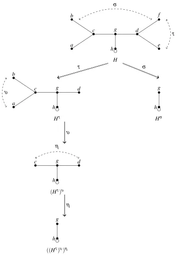
Example 3.6. InFigure 1we give an example of a graph H, along with two ways of reducingH by
involutions. On the right-hand side we reduceHby using the involutionσ that swaps each of the pairs
of verticesaande, band f,c andd, leaving behind only the involution-free graph on the verticesg andh. On the left-hand side, we begin with the involutionτ that swapseand f, and have to reduce the
resulting graph by involutions twice more before we get to the involution-free graph((Hτ)υ)η, which is isomorphic to the graphHσ. This is not a coincidence. We will see inTheorem 3.7that reduced forms are unique.
To make further progress, we need to assumek=pis prime. Eventually, we will further restrict attention to the casep=2. However, we state and prove some intermediate results for a general primep, as they may be of use in further explorations of modular counting problems.
Theorem 3.4says that in classifying the complexity of #pH-COLOURINGproblems, it is enough to
restrict attention to graphsHthat are reduced forms, i. e., that do not have any automorphisms of order p. This is enough for the proof of the main dichotomy result, but it is an interesting fact that reduced forms are unique. In any case, the concepts used in the proof of uniqueness of the reduced form will be needed later.
Theorem 3.7. Given a graph G, and a prime p there is (up to isomorphism) exactly one graph G∗such
that G∗has no automorphisms of order p and G→∗pG∗.
The proof is deferred to the next section. We can now state main result.
Theorem 3.8. If H is a tree, then⊕H-COLOURING is⊕P-complete if the reduced form obtained by
reducing H by involutions is non-trivial, i. e., has more than one vertex. Otherwise it is solvable in polynomial time.
We conjecture that this result holds for graphs in general. The conjecture is unresolved, though Göbel, Goldberg and Richerby [10] recently extended our result from trees to cactus graphs. One could extend the conjecture to #pH-COLOURING, for primes p>2. Specifically, one might conjecture that, for eachp,
the set of reduced formsH corresponding to polynomial-time cases of #pH-COLOURINGis finite (and
that all other reduced forms correspond to#pP-complete cases). However, we do not go that far here.
3.2 The Lovász vector of a graph
We need a modular version of the Lovász vector [14, §2.3] of a graph.
Definition 3.9. Letpbe a prime, andG1,G2, . . .be a fixed enumeration of all pairwise non-isomorphic graphs. (Thus every graph is isomorphic to exactly one graph in the sequence.) Themod-p Lovász vector of a graphHis the sequence([hom(Gi,H)]p:i≥1).
a b
c g d
e f
h σ
τ
H τ
υ
η
σ
a b
c g d
h υ
Hτ
g
h
Hσ
c g d
h η
(Hτ)υ
g
h
((Hτ)υ)η
of orderp. For the statement and proof of the classical (non-modular) version ofLemma 3.10below, see [18, Problem 15.20(b)]. Note that the ideas were generalised by Lovász to a much wider setting [17]. First recall the following fact about finite groups. For any primep, a finite groupGhas an element of orderpif and only if the order ofGis divisible byp. (In the context of group theory, the “if” direction is Cauchy’s theorem and the “only if” Lagrange’s theorem.)
Lemma 3.10. Suppose p is a prime, and H and H0are two graphs, neither of which has an automorphism
of order p. Then H and H0are isomorphic if and only if they have the same mod-p Lovász vector.
Proof. Clearly the condition is necessary: two isomorphic graphs have the same mod-pLovász vector. Now we need to prove that it is sufficient. This proof is similar to the proof of Theorem 2.11 in Hell and Nešetˇril’s monograph [15].
So supposeHandH0have the same mod-pLovász vector, that is,
hom(G,H)≡hom(G,H0) (mod p), (3.1) for all graphsG. We first observe that, in order to show thatHandH0are isomorphic, it is sufficient to prove that for every graphG,
inj(G,H)≡inj(G,H0) (mod p), (3.2) where inj(G,H)denotes the number of injective homomorphisms fromGtoH. To see this, first take G=H in the above congruence (3.2). The left hand side of the congruence is just the order of the automorphism group ofH, which, sinceH does not have an automorphism of orderp, is not congruent to 0modulo p. Therefore, the right hand side, inj(H,H0), is also different from from 0modulo pand, in particular, there exists an injective homomorphism fromHtoH0. Similarly, if we takeG=H0we find an injective homomorphism the other way, and thus an isomorphism betweenHandH0.
We will prove that the system of congruences (3.1) implies the system (3.2), by induction onn, the number of vertices ofG. Specifically, our induction hypothesis is that if congruence (3.1) holds for all graphsGwithnor fewer vertices, then the same is true of congruence (3.2). Ifn=1, thenGhas only one vertex and every homomorphism fromGto any other graph is injective and (3.2) holds.
Now assumen>1. For a partitionΘ={Si:i∈I}of the vertex setV(G)of a graphG, define the
quotient graphG/Θas follows. The vertex set ofG/Θis the index setI. There is an edge betweeni,j∈I inG/Θiff there is some edge joining a vertex inSito a vertex inSj inΘ. (It may happen thati= j, in
which caseG/Θhas a loop ati.) A colouring ofGwithHinduces a partition ofGin the obvious way, with vertices which are given the same colour assigned to the same part of the partition. If we call this partitionΘ, then anyH-colouring ofGcan be considered as an injectiveH-colouring ofG/Θ, since each vertex ofG/Θis associated with exactly one colour fromH. Letιbe the partition consisting of a single
block for each vertex (i. e., the partition associated with injective homomorphisms fromGtoH). Then we have both
hom(G,H) =inj(G,H) +
∑
Θ6=ι
inj(G/Θ,H) and
hom(G,H0) =inj(G,H0) +
∑
Θ6=ι
SinceG/Θis necessarily smaller thanGifΘ6=ι, we know by the induction hypothesis that inj(G/Θ,H)≡ inj(G/Θ,H0) (mod p), and since hom(G,H)≡hom(G,H0) (mod p)by assumption, we do indeed have inj(G,H)≡inj(G,H0) (mod p), as required.
Note that the largest graphGconsidered in the above inductive argument has the same number of vertices asH. So ifHandH0 are not isomorphic then there must be a graphGwith at most as many vertices asHthat distinguishesHandH0, that is, hom(G,H)6≡hom(G,H0) (mod p).
Proof ofTheorem 3.7. SupposeG→∗pG∗andG→∗pG†, whereG∗andG†have no automorphisms of orderp. Theorem 3.4says the reduction operation→ppreserves the mod-pLovász vector, soG∗and G† have the same vector. On the other hand, Lemma 3.10above says that the mod-pLovász vector characterises (isomorphism classes of) graphs with no automorphisms of order p, soG∗ andG† are isomorphic.
4
Pinning colours to vertices
We would like to be able to count the number ofH-colourings of a given graphG in which certain vertices ofGare forced to receive certain colours fromH. This would allow us to isolate a suitable “hard” subgraph H0 ofH, and hence reduce the known hard H0-colouring problem to the particular H-colouring problem that interests us. We achieve this by building gadgets, which are graphs with a distinguished vertex, with the following property: effectively, only a certain set of colours can be applied to the distinguished vertex of a gadget. By attaching these gadgets to a vertex ofG, we can restrict that vertex to be coloured with a particular set of colours.
4.1 Rooted graphs
Definition 4.1. Arooted graphis a pair(G,v)whereGis a graph andv∈V(G)is a distinguished vertex ofG(referred to as theroot).
In essence, we want to show that for any two distinct coloursh1,h2∈V(H)in a givenH, there exists
some rooted graph(Γ,γ)such that the number of ways ofH-colouringΓwithγreceivingh1is different,
modulo2, to the number of ways ofH-colouringΓwithγreceivingh2. (In fact, as we can see, we can
find such a rooted graphΓfor all prime moduli.) SupposeGis an instance graph with distinguished root vertexv. We can then use rooted graphs such as(Γ,γ)to pick out the colourings ofGin which vertexv
receives a colour from some particular subset of the colours. Roughly, we do this by attaching a copy of ΓtoG, identifyingγandv. Call the resulting graphG0. Suppose a colouring ofGwith vertexvreceiving h1extends to a colouring ofG0in (say) an odd number of ways. Then a colouring withvreceivingh2will
extend in an even number of ways. In this way we have effectively “cancelled” the colourings ofGwithv colouredh2, while leaving untouched those withvcolouredh1.
The construction of the required gadgets rests on a rooted version ofLemma 3.10. Before we give the proof, we need to define rooted versions of a few concepts we have already encountered.
Definition 4.2. A homomorphism(repectively, isomorphism) between two rooted graphs (G,v)and
Definition 4.3. We denote the number of homomorphisms from rooted graph (G,g) to rooted graph
(H,h)by hom∗((G,g),(H,h)). If the roots are implied by the context we will sometimes suppress them in the above notation, and just write hom∗(G,H).
Similarly, we denote the number of injective homomorphisms from rooted graph(G,g)to(H,h)by inj∗((G,g),(H,h))and, again, we may suppress the specified vertices if they are implied by the context, instead writing inj∗(G,H).
Finally, we will use the concept of the Lovász vector of a rooted graph.
Definition 4.4. LetG1,G2, . . .be a fixed enumeration of all pairwise non-isomorphic rooted graphs. Then the mod-pLovász vector of a rooted graphHis the sequence([hom∗(Gi,H)]p:i≥1).
We will useparity Lovász vectoras an alternative name for mod-2 Lovász vector.
Lemma 4.5. Suppose p is a prime, and H and H0 are two rooted graphs neither of which has an
automorphism of order p. Then H and H0are isomorphic if and only if they have the same mod-p Lovász vector.
Proof. As forLemma 3.10, but with hom∗and inj∗replacing hom and inj. In defining the quotient of a rooted graph(G,g)by a partitionΘ={Si:i∈I}, we define the root of(G,g)/Θto be the vertexi∈I
such thatg∈Si.
As withLemma 3.10, it can be seen that we need only finitely many terms of the mod-pLovász vector to reconstruct(H,h).
4.2 Building gadgets
In the following we return to⊕H-COLOURING, and are only interested in automorphisms of order two, or
involutions. Note that many of the results in this section can be generalised to automorphisms of arbitrary prime order, but we only require the gadgets for the casep=2 inSection 5, so only this case is presented here, for simplicity.
It will be useful to consider the case whereHandH0have the same underlying graph but different roots (note that forHandH0to be non-isomorphic as rooted graphs, there can be no automorphism ofH with takeshtoh0, i. e., thathandh0lie in different orbits of the automorphism group ofH). Since we will no longer be able to use the previous naming convention for the specified vertices, we will refer to the two roots inH asxandy. In the following, we will be assuming thatH(as an unrooted graph) is involution-free. As we saw inSection 3, it suffices to consider the complexity of⊕H-COLOURINGfor involution-freeH.
Lemma 4.5allows us to construct the following useful gadgets: given an involution-free graphH and two colours x andy which are in different orbits of Aut(H), there is a rooted graph (Γ,γ) that
distinguishesxandy.
Lemma 4.6. Given an involution-free graph H and two vertices x and y which lie in different orbits of
Proof. Since(H,x)and(H,y)are non-isomorphic as rooted graphs, they have different parity Lovász vectors byLemma 4.5. Simply take(Γ,γ)to be the first rooted graph for which the corresponding entries
of the parity Lovász vectors of(H,x)and(H,y)differ.
We will use rooted graphs such as those guaranteed byLemma 4.6as “gadgets” in a reduction from the problem of counting restrictedH-colourings (in which a given vertex of the instance graph is forced to be coloured with colours from a specified orbit of Aut(H)) to the problem of counting unrestricted H-colouringsmodulo2.
Theorem 4.7. Given an involution-free graph H, an orbit O of the automorphism group of H, and an
oracle for⊕H-COLOURING, it is possible to determine, in polynomial time, the parity of the number of
H-colourings of a rooted graph G in which the root receives a colour from O.
Note that this result would follow immediately if we were able to build a gadget (i. e., rooted graph)
(Γ,γ)such that hom∗((Γ,γ),(H,x))is odd, while hom∗((Γ,γ),(H,y))is even for ally6=x. Then we
could just attach a copy ofΓat the vertex ofGthat we want to colour withx, identifying this vertex withγ, and then countH-colourings of the new graph. Unfortunately,Lemma 4.6doesn’t allow us to
construct such a gadget, as it doesn’t allow us to choose which colour isxand which isy. However, we can construct a series of gadgets that allow us to count colourings ofGin which the root ofGreceives a colour from a given orbit ofH, by developing a sort of algebra on the gadgets, as described below.
Definition 4.8. SupposeHis a graph, andh1, . . . ,hnis an enumeration of the vertices ofH. With each
gadget(Γ,γ)we associate a vectorvH(Γ)∈GF(2)n, indexed by{1, . . . ,n}, such that theithcomponent
of the vector is 1 if there are an odd number ofH-colourings ofΓthat use colourhiatγ, and 0 otherwise.
Note that if two colours (vertices ofH)hiandhjare in the same orbit of the automorphism group ofH
then theithand jthentries ofvH(G)are the same for all rooted graphsG. So we may instead consider the
vectorv∗H(G)which is indexed byorbitsof the automorphism group ofHrather than individual vertices ofH, the coordinate ofv∗H(G)associated with a given orbit being the coordinate ofvH(G)associated
with any (and hence all) of the colours in that orbit. Note thatvH(G)andv∗H(G)contain exactly the same
information.
We define an operation that combines two rooted graphs by identifying their root vertices.
Definition 4.9. Given two rooted graphsΓandΠ, we define the the new rooted graphΓ·Πto be the
graph obtained by identifying the roots of each. The root ofΓ·Πis the vertex formed by identifying the roots of the other two graphs.
If we think of each gadgetΓandΠas enforcing a certain set of allowed colours at its root vertex, we can view this operation as forming a gadget that enforces the intersection of these sets. This is equivalent to saying that vectorvH associated with the new gadget is obtained by taking the coordinate-wise product
of the vectors associated with the individual gadgets.
Lemma 4.11. SupposeΓandΠare two rooted graphs, and H is graph. Then vH(Γ·Π) =vH(Γ)∗vH(Π). Proof. Fix a colourhi∈V(H). The number of colourings ofΓ·Πwith the root receiving colourhiis just
the product of the number of colouringsΓandΠwith the roots in each case receiving colourhi. Thus, if
there is a zero in theithplace of either of the vectorsvH(Γ)orvH(Π), then there is a zero in theithplace ofvH(Γ·Π); otherwise there is a one.
We now introduce a formal sum of rooted graphs, with coefficients in GF(2), which preserves addition of these vectors. Note that since this sum has coefficients in GF(2)we haveΓ+Γ=0.
Definition 4.12. For a set of rooted graphsΓ1,Γ2,· · ·,Γr, we definevH(Γ1+Γ2+· · ·+Γr)to bevH(Γ1) +
vH(Γ2) +· · ·+vH(Γr).
Definition 4.13. We will say that a vectorv∈GF(2)nisimplementablefor somen-vertexHif there is a
set of rooted graphs{Γ1,Γ2, . . . ,Γr}such thatvis equal tovH(Γ1+Γ2+· · ·+Γr).
Supposevis the characteristic vector of a set of colours we wish to restrict to, as in the discussion followingTheorem 4.7. We’ll see presently that the gadgetsΓ1, . . . ,Γrwill enable us to effectively restrict
to that colour set, justifying the term “implementable”.
Lemma 4.14. The set of vectors that are implementable for a given H is closed under the operations of
vector addition and point-wise multiplication (or the operation∗, as defined inDefinition 4.10).
Proof. Supposev=vH(Γ1+Γ2+· · ·+Γr)andv0=vH(Π1+Π2+· · ·+Πs)are any two implementable
vectors. Thenv+v0is implementable, since
v+v0=vH(Γ1+Γ2+· · ·+Γr+Π1+Π2+· · ·+Πs).
Furthermore, noting that∗distributes over+,
v∗v0=vH(Γ1+Γ2+· · ·+Γr)∗vH(Π1+Π2+· · ·+Πs)
= vH(Γ1) +vH(Γ2) +· · ·+vH(Γr)
∗ vH(Π1) +vH(Π2) +· · ·+vH(Πs)
=vH(Γ1)∗vH(Π1) +vH(Γ1)∗vH(Π2) +· · ·+vH(Γr)∗vH(Πs)
=vH(Γ1·Π1) +vH(Γ1·Π2) +· · ·+vH(Γr·Πs) (4.1)
=vH(Γ1·Π1+· · ·+Γr·Πs),
where equality (4.1) follows from repeated application ofLemma 4.11.
Lemma 4.15. For any involution-free graph, H, the all-ones vector is implementable, and for any pair of
distinct orbits in H there is at least one implementable vector that has a 1 at every vertex in one of the two orbits and a 0 at every vertex in the other orbit.
Proof. The all-ones vector is implementable using the graph on one vertex. The rooted graphs whose vectors distinguish between distinct orbits of colours inHare obtained usingLemma 4.6.
Lemma 4.16. Consider a set, S, of vectors inGF(2)nwhich contains the all-ones vector(1,1, . . . ,1)and has the property that for any two indices i and j there is some vector in the set whose ithcoordinate differs from its jthcoordinate. The closure of this set under the operations of coordinate-wise multiplication and coordinate-wise addition includes each of the vectors in the standard basis.
Proof. We proceed by induction onn. Ifn=1 the lemma clearly holds, as the all-ones vector is the only vector in the standard basis. Now, assume thatn>1; we shall attempt to construct the vectors in the standard basis in GF(2)n.
By induction, we can construct vectors that agree with the standard basis in the firstn−1 places, without being able to control what happens in thenthplace (note that the restriction of the set of vectorsS to the firstn−1 places still satisfies the conditions of the lemma). That is, we can certainly obtain vectors of each of the following forms, where thexican be either 0 or 1
(1 1 1 1 . . . 1 1 1) (1 0 0 0 . . . 0 0 x1) (0 1 0 0 . . . 0 0 x2)
(0 0 1 0 . . . 0 0 x3)
..
. ...
(0 0 0 0 . . . 0 1 xn)
This leaves several cases:
Case 1. Thexi are all equal to zero. In this case, we already have the firstn−1 vectors from the
standard basis, and we can just take the sum of alln−1 vectors with the all-ones vector, which has a 1 in the last place and zeros everywhere else, to get the last one.
Case 2. There are at least twoi,jsuch thatxi,xj=1. But then the product of these two vectors is the
vector(0,0, . . . ,0,1). To obtain the remaining vectors from the standard basis, we just take the sum of this vector with any of those from the original list which had a 1 in thenthplace, i. e.,ei is the sum of this
vector with the vector that had a 1 in theithplace and a 1 in thenth place.
Case 3. There is exactly one vector in the list,vwith a 1 as thenthcoordinate. Say this vector has a 1 in theithandnth places. By assumption, there is some vector inSwhich has different values in thenth andithplaces. The product of this withvis a vector with exactly one 1, in either theithor thenthplace, and the sum of this basis vector withvis the other ofeianden.
Lemma 4.17. For any involution-free graph H, and any orbit of O ofAut(H), the characteristic vector of O (which is 1 in coordinates indexed by O and 0 elsewhere) is implementable.
Proof. For the purposes of this proof, it is convenient to think in terms to the abbreviated vectorsv∗H(G)
in place of the full vectorsvH(G). (This is not an essential change; we are merely eliminating duplicated
coordinates.) So, now, an implementable vector is one the formv∗H(Γ1+· · ·+Γr), for some rooted graphs
Γ1, . . . ,Γr. ByLemma 4.14the set of vectors we can implement is closed under the operations of addition
and coordinate-wise multiplication, and byLemma 4.15we can implement the all ones vector and, for each pair of indices (orbits)iand ja vectorvwithvi6=vj. Thus, byLemma 4.16, every vector in the
We are now ready to return toTheorem 4.7. Letvbe the characteristic vector of the orbitO. We know thatvis implementable. So we now just have to show that our definition of “implementable” actually does what we want it to do. That is, it is possible to determine, in polynomial time using an oracle for unrestrictedH-colourings, the parity of the number ofH-colourings of a rooted graphGin which the root receives a colour fromO.
Proof ofTheorem 4.7. Letv∈GF(2)nbe the characteristic vector of the orbitO. ByLemma 4.17, the vectorvis implementable, i. e.,v=vH(Γ1+Γ2+· · ·+Γr)for some set of rooted graphs{Γ1, . . . ,Γr}.
Thus,
vH(G)∗v=vH(G)∗vH(Γ1+Γ2+· · ·+Γr)
=vH(G)∗vH(Γ1) +· · ·+vH(G)∗vH(Γr)
=vH(G·Γ1) +· · ·+vH(G·Γr).
Now take the sum of the coordinates of the vectors,modulo2:
n
∑
i=1
(vH(G)∗v)i= n
∑
i=1
vH(G·Γ1)i+· · ·+ n
∑
i=1
vH(G·Γr)i.
The left-hand side counts,modulo2,H-colourings ofGin which vertexxreceives a colour fromO; this is exactly the quantity we are interested in computing. The jthterm on the right hand side, counts, modulo2, the number of (unrestricted)H-colourings of the graphG·Γj. So the right-hand side can be
evaluated usingrcalls to an oracle for⊕H-COLOURING.
Finally, we need an analogue ofTheorem 4.7which allows pinning of two vertices ofG. (We thank the authors of [10] for pointing out a lacuna at this point in an earlier version of the proof.)
Corollary 4.18. Suppose G is a graph with distinguished vertices x and y. Given an involution-free
graph H, orbits O and O0of the automorphism group of H, and an oracle for⊕H-COLOURING, it is possible to determine, in polynomial time, the parity of the number of H-colourings of G in which x (respectively y) receives a colour from O (respectively O0).
Proof. Define the matrixA= (ai j)∈GF(2)n×nas follows. For all 1≤i,j≤n, ai j=
number of colourings ofGwithxreceiving colouriandycolour j2.
Let u and v be the characteristic vectors of Oand O0. By Lemma 4.17 we know that u and v are implementable, i. e.,u=vH(Γ1) +· · ·+vH(Γr)andv=vH(Γ01) +· · ·+vH(Γ0s)for some rooted graphs
Γ1, . . . ,ΓrandΓ01, . . . ,Γ0s. Thus
u|Av≡ vH(Γ1) +· · ·+vH(Γr) |
A vH(Γ01) +· · ·+vH(Γ0s)
≡ r
∑
i=1 s
∑
j=1
vH(Γi)|A vH(Γ0j) (mod 2).
Note that the left hand side is the quantity we are interested in, namely the number of restrictedH -colourings ofG. Finally note that the(i,j)thterm in the last sum is equal,modulo2, to the number of colourings ofGwithΓiattached toxandΓ0j toy. So each term on the right hand side may be computed
5
Trees
As we have seen, applying the reduction operations inDefinition 3.5preserves the parity of the number of H-colourings of any graphG. This allows us to concentrate on involution-free graphs. There are certain involution-free graphsHfor which theH-colouring problem obviously lies inP:
- the null graph (the graph on no vertices),
- the graph on one vertex with no loop, - the graph on one vertex with a loop, and
- the graph on two disconnected vertices, one with a loop and one without.
(5.1)
Lemma 5.1. If H is one of the graphs in list5.1, then H-colourings of an instance G can be counted in
polynomial time.
Proof. IfHis the null graph then there is noH-colouring ofG, so the counting problem is obviously trivial. IfHis the graph on one vertex thenGhas exactly oneH-colouring if and only ifGhas no edges, and zero otherwise, which can be determined in polynomial time. IfHis the graph on one vertex with a loop, then there is exactly oneH-colouring ofG. IfHis the graph on two vertices one with a loop and one without then there are exactly 2|Isol(G)|colourings ofG, where Isol(G)is the set of isolated vertices ofG. Each isolated vertex can be coloured with either the looped vertex or the unlooped vertex ofH independently, and all the vertices which form part of a connected component of size greater than one must be coloured with the looped vertex.
Corollary 5.2. Let H0be the reduced form associated with H in the reduction system defined in
Defini-tion 3.5. If H0is one of the graphs in list5.1, then⊕H-COLOURINGis inP.
Proof. This follows directly fromLemma 5.1and the fact that the reduction system preserves the parity of the number ofH-colourings, as shown inLemma 3.3
We conjecture that for general graphs, the criterion given inCorollary 5.2, that is,Hreducing by involutions to one of the four trivial graphs, is the only way in which the⊕H-COLOURINGproblem can fail to be⊕P-complete. Note that this criterion does encompass all of the easy cases identified by Dyer and Greenhill [6]. A complete graph with loops everywhere reduces to the null graph if it has an even number of vertices and the graph on one vertex with a loop if it has an odd number. On the other hand, a complete bipartite graph reduces to the graph on one vertex if there are an odd number of vertices in total, and the null graph otherwise.
In this section, we will prove that this conjecture is true for trees. In particular, if, in the reduction system ofDefinition 3.5, the reduced form associated with a given treeT has at most one vertex, then the associated⊕T-COLOURINGproblem can be solved in polynomial time. Otherwise, it is⊕P-complete.
5.1 Involution-free trees
Involution-free trees have quite a lot of structure, and we will exploit this when we build gadgets for our reductions from⊕INDSET(defined below) to⊕H-COLOURINGin the next section.
Lemma 5.3. An involution-free tree on more than one vertex has two vertices of degree 2 which are
adjacent to leaves.
Proof. The argument given below is very similar to the standard argument given to show that any tree has at least two leaves.
The first observation to make is that any involution-free tree contains some path of length at least 3. If the maximum-length path in a tree is of length 1, then the tree consists of a single edge, and so has an involution. If it is of length 2, then the tree is a star, and exchanging any two of its leaves is an involution.
Consider a longest path in an involution-free tree, and label the vertices of this path p0,p1, . . . ,p`.
Note thatp0and p`are both leaves. Then we claim that both vertices p1and p`−1are degree 2. Note
thatp1and p`−1are in fact distinct vertices, as`≥3. Assume the degree of p1is greater than 2, and
consider a vertex,v, adjacent top1, which is neitherp0norp2. This vertex cannot have any neighbours
which are not already in the path (as this would contradict maximality of the path). It also cannot have any neighbours which are in the path (as this would create a cycle, contradicting the fact thatGis a tree). Therefore, it cannot have any neighbours other thanp1. But then exchanging this vertex withp0is an
involution ofG, so there is no such vertex, andp1is degree 2 as claimed. An analogous argument shows
thatp`−1must be degree 2.
We will also require the following lemma.
Lemma 5.4. An involution-free tree has trivial automorphism group.
Proof. The automorphism group of a tree can be formed from symmetric groups using the operations of direct product and wreath product with a symmetric group (Pólya [20] after Jordan [16]). Since the symmetric groupsSnforn>1 have even order, the automorphism group of a tree is either of even order
or has order 1. If it has even order, then the tree has an involution.
Finally, we require the following technical lemma concerning the number of walks (i. e., not necessar-ily simple paths) of various lengths between vertices in involution-free trees. Note that the verticese0 ande`mentioned in the statement of the lemma are guaranteed byLemma 5.3.
Lemma 5.5. Let H be an involution-free tree, let e0be a vertex of degree 2 that is adjacent to a leaf in H,
and let e`be a vertex of even degree such that there are no vertices of even degree on the path joining e0
and e`, where`≥1is the length of the path joining e0 and e`. We will name the vertices on this path
e0,o1,o2, . . . ,o`−1,e`.
Then there are an even number of vertices v such that both:
1. v is a neighbour of the first vertex on this path other than e0, i. e., v is a neighbour of e1in the case `=1, and a neighbour of o1otherwise; and
Proof. We will refer in this proof to the verticeso1ando2, which do not exist if`=1 or`=2, we deal
with this at the end of this proof. For now, assume`≥3. We want to prove that there are an even number of neighbours ofo1from which there are an odd number of walks of length`toe`inH. There are an odd
number of paths of length`frome`to each of the neighbours ofo1other thano2: there is, in fact, one
such walk, and it is the unique path connecting the neighbour toe`in the tree. We claim that there are an
even number of walks of length`frome`too2.
A walk of length`frome`too2traverses exactly 1 edge more than once, as there is a unique path of
length`−2 frome`too2. Two such walks which traverse the same edge more than once are identical.
There is therefore a one-to-one correspondence between these walks and the edges which are traversed at least twice by at least one of them. We claim that the number of such edges is even.
Any edge which is adjacent to any of the vertices in{o2,o3, . . . ,e`}, and only those edges, may be traversed more than once, so it suffices to show that there are an even number of such edges. To see this, note that the only edges in this set which are adjacent to more than one of the vertices in the set are:{(o2,o3),(o3,o4), . . . ,(o`−1,e`)}, there are the same number of edges in this set as the number of
vertices of odd degree in{o2, . . . ,e`}. The total number of edges is then just the sum of the vertex degrees
minus the number of edges which are adjacent to more than one of the vertices; but the sum of the vertex degrees is`−2 (mod 2)(as there are`−2 vertices of odd degree) and the number of repeated edges is
`−2, so the parity of the total number of edges is(`−2)−(`−2)≡0 (mod 2).
As noted above, if`=1 or if`=2 the verticeso1oro2may not exist. However, the theorem still
holds.
In particular, if`=1 then we actually have two adjacent vertices of even degree and the first vertex on the path which is note0is in facte1, which is of even degree. Clearly there are an even number of
vertices adjacent toe1with an odd number of length 1 walks toe1, these being exactly the neighbours of e1.
If`=2, then again the vertex whose neighbours we are interested in is of odd degree, call ito1, and
there are an odd number of walks of length 2 frome2to each of the neighbours ofo1other than itself: in
fact, there is exactly one such walk, the path joining the two vertices. On the other hand,e2is of even
degree, so there are an even number of walks of length 2 frome2to itself. Sinceo1has an odd number of
neighbours, this leaves an even number of neighbours ofo1which have an odd number of length 2 walks
toe2, as claimed.
5.2 The reduction
Our starting point is the following problem, which was shown by Valiant [22] (in the guise of “Mon 2-CNF”) to be⊕P-complete; see also Faben [8, Thm. 3.5]).
Name. ⊕INDSET.
Instance. An undirected graphG.
Output. The parity of the number of independent sets inG.
Theorem 5.6. Given an involution-free tree H with more than one vertex,⊕H-COLOURING is ⊕P
G σ2(G)
Figure 2: The 2-stretch ofG.
Definition 5.7. Given a graphG, we callσ2(G)the graph obtained by replacing every edge inGwith a
path of length 2. We refer to the newly introduced vertices asstretch vertices, and the original vertices of GasG-vertices. The construction is illustrated inFigure 2.
The graph defined above,σ2(G), is usually referred to as the2-stretchofG, and it is an established
result that countingH-colourings ofσ2(G)is equivalent to countingH2-colourings ofG, whereH2is
the multigraph whose adjacency matrix is the square of the adjacency matrix ofH(see, e. g.,[6]). We will use a variant of this stretch operation in which we count only those colourings ofσ2(G)in which
both the stretch vertices and theG-vertices are coloured with specific subsets of the colours inH. This is achieved using gadgetry based on the principles established inSection 4.
We now detail the reduction from⊕INDSET. First, given any graphG, we will construct a certain graphG∗. We then claim that the number ofH-colourings ofG∗, with certain vertices restricted to receive certain colours fromH, is congruentmodulo2 to the number of independent sets inG.
For a given involution-free treeH, pick a vertex of degree 2,e0, adjacent to a leaf, and a vertex of
even degree,ek such that the unique path of lengthkinHfrome0toek does not contain any vertex of
even degree (exactly as in the statement ofLemma 5.5). Note that, asH is involution-free, there are two vertices of even degree, and at least one vertex of degree two which is adjacent to a leaf inHby
Lemma 5.3, and we can choosee0andekwith the above properties.
Now, given a graphG, first createσ2(G), then add two new verticesRandB. Add an edge between
each of the original vertices ofG(G-vertices) andR, and a path of lengthkfrom every one of the new vertices (stretch vertices) ofσ2(G)toB. We call this new graphG∗, and the construction is illustrated in Figure 3.
Now, using the technology described inCorollary 4.18, and the fact that the orbit of a vertex in an involution-free tree is trivial byLemma 5.4, we can determine the parity of the number ofH-colourings ofG∗, in whichRis restricted to be coloured withe0andBis restricted to be coloured withek, using
only a⊕H-COLOURINGoracle. We claim that this number is congruent (modulo2) to the number of independent sets inG. We will use what we know about the number of walks of lengthkbetween the colourse0andekfromLemma 5.5.
Lemma 5.8. Suppose H is an involution-free tree, and let e0be a vertex of degree 2 adjacent to a leaf,
R G B
Figure 3: The construction ofG∗.
the path of length k joining them. Suppose G is a graph and let G∗be constructed from G as described above.
Then the number of H-colourings of G∗ in which R receives e0 and B receives ek is congruent modulo 2 to the number of independent sets in G.
Proof. First consider theG-vertices inG. They are all neighbours of a vertex which is coloured with e0, so they must therefore receive colours that are adjacent toe0inH. Bute0was chosen to be one of
the vertices of degree 2 adjacent to a leaf inH, soG-vertices can only be coloured with either the leaf adjacent toe0(which we will calll) or with the first vertex on the path linkinge0andek, which we will
callv1in the remainder of this proof. This vertex iso1, except in the casek=1 where it ise1.
Now, consider the stretch vertices. These are connected to a vertex which is colouredekby a path of
lengthk. So, consider the colour used at a given stretch vertex,s. If there are an even number of walks of lengthk fromek to this colour inH, then there are an even number of colourings ofG∗ which use
that colour ats, as there are an even number of ways of colouring the path joiningsandB, and the total number of colourings is the product of the number of ways of colouring this path with the number of ways of colouring the rest of the graph.
We therefore need to count colourings ofG∗in which the colours used at the stretch vertices are such that there are an odd number of paths of lengthkbetween them andek inH. Note that these colours
must also be adjacent to eitherv1 orlinH (as theG-vertices are all coloured with eitherv1orl, and every stretch vertex is adjacent to aG-vertex), and therefore, in fact, must be adjacent tov1, as the only
neighbour oflise0, which is also a neighbour ofv1.
Now, we are reduced to considering colourings ofG∗in which the following conditions hold. The G-vertices are coloured eitherlorv1, while the stretch vertices are coloured with one of the neighbours ofv1which has an odd number of lengthkwalks from itself toek. We claim that the parity of the number
of such colourings is equal to the parity of the number of ways of colouringGwith the two coloursland v1such that no two vertices coloured withv1are adjacent.
Consider a colouring ofGwith the coloursv1andl. If there are two vertices ofGwhich are adjacent inGand both coloured withv1 then there are an even number of extensions of this colouring to an
byLemma 5.5.
On the other hand, if there are no two such vertices, there is exactly one extension of the given colouring ofGto anH-colouring ofG∗: every one of the stretch vertices is adjacent to a vertex which is colouredl, so the stretch vertices must all be colourede0, and as there is only one path of lengthkfrom
e0toekinH, this determines the colouring of the vertices on the paths linking the stretch vertices toB.
So the number of colourings ofG∗withHsuch thatRis colourede0andBis colouredekis congruent modulo2 to the number of colourings ofGin which each vertex is either coloured with lorv1 and
adjacent vertices may not both be coloured withv1. But these are exactly the independent sets ofG:
vertices colouredv1are “in” the independent set and vertices colouredlare “out”.
Proof ofTheorem 5.6. ByTheorem 4.18andLemma 5.4we can countH-colourings ofG∗in whichR is colourede0andBis colouredek in polynomial time if equipped with anH-colouring oracle. But we
know that the number of such colourings is congruentmodulo2 to the number of independent sets inG. Since clearlyG∗can be constructed fromGin polynomial time, this gives us a polynomial-time Turing reduction from⊕INDSETto⊕H-COLOURING.
5.3 A dichotomy for trees
The main result now follows easily.
Proof ofTheorem 3.8. ByLemma 3.3, the number ofH-colourings of a graphGis congruentmodulo 2 to the number ofH0-colourings, whereH0 is any graph obtained fromH by reducingH by any of its involutions. Also, ifH is a tree then any graphH0 which can be reached fromH by reduction by involutions is also a tree. It therefore suffices to consider involution-free trees.
If H is an involution-free tree, andH contains more than one vertex, then Theorem 5.6 shows that⊕H-COLOURING is⊕P-complete. On the other hand, ifH contains either 0 or 1 vertices then #H-COLOURING(and hence⊕H-COLOURING) is polynomial-time solvable byLemma 5.1.
Note that the dichotomy described byTheorem 3.8is decidable in polynomial time.
6
Other graphs
As noted earlier, we conjecture not only that there is a dichotomy for the complexity of⊕H-COLOURING
for generalH, but that this dichotomy arises in the same way as it does for trees. In other words, that the only way in which a⊕H-COLOURINGproblem can be polynomial-time solvable is ifHreduces by involutions to one of the four trivial graphs. If this is the correct characterisation, then the dichotomy is certainly decidable, but it is not clear whether it can be decided in polynomial time. On the face of it, finding the reduced form associated with a graphH requires finding an involution ofH, and no polynomial-time algorithm is known for this problem.
We finish by showing that in uncovering a dichotomy for general graphs it is enough to consider connectedH. That is, if an involution-free graphHhas any connected componentH1for which⊕H1
Theorem 6.1. Let H be an involution-free graph. If H1 is a connected component of H and ⊕H1
-COLOURINGis⊕P-hard, then⊕H-COLOURINGis⊕P-hard.
Proof. Take any graphG, and assume thatGis connected (since the number ofH-colourings ofGis just the product of the number ofH-colourings of each of its connected components). We can use an oracle forH-colouring to determine the parity of the number of colourings ofGin which only colours fromH1 are used in the following way: letv∈V(G)be any vertex ofG. For each colourhi∈V(H1), we can count
the colourings ofGin whichvis colouredhiusingTheorem 4.7. Notice that the size of the orbit ofhiin
Aut(H)is odd, asHhas no involutions, so the parity of the number of colourings ofGwithhi atvis the
same as the parity of the number of colourings ofGwhich use any of the vertices in the orbit ofhiatv.
But we can do this for every vertex inH1, and sinceGis connected, any colouring which uses a vertex fromH1atvcan use only colours fromH1anywhere inG. Conversely, any colouring ofGwhich uses
only colours fromH1must use some colour fromH1atv, so this does indeed allow us to count all such
colourings ofG.
Note that this actually allows us to strengthenTheorem 3.8: theH-colouring problem associated with anyforest His polynomial-time solvable if the reduced form associated with the forest in the reduction system described inSection 3is the null graph or the graph on one vertex, and⊕P-complete otherwise.
References
[1] ANDREIA. BULATOV: The complexity of the counting constraint satisfaction problem. J. ACM, 60(5):34, 2013. Preliminary version inICALP’08, also available atECCC. [doi:10.1145/2528400]
36
[2] ANDREI A. BULATOV AND MARTIN GROHE: The complexity of partition functions.
Theoret. Comput. Sci., 348(2-3):148–186, 2005. Preliminary version in ICALP’04. [doi:10.1016/j.tcs.2005.09.011] 36
[3] JIN-YI CAI AND XI CHEN: Complexity of counting CSP with complex weights. In Proc. 44th STOC, pp. 909–920, New York, 2012. ACM Press. [doi:10.1145/2213977.2214059,
arXiv:1111.2384] 36
[4] JIN-YI CAI, XI CHEN, AND PINYAN LU: Graph homomorphisms with complex values: A dichotomy theorem. SIAM J. Comput., 42(3):924–1029, 2013. Preliminary versions inICALP’10
andarXiv. [doi:10.1137/110840194] 36
[5] XICHEN: Guest column: Complexity dichotomies of counting problems. SIGACT News, 42(4):54– 76, 2011. [doi:10.1145/2078162.2078177] 36
[7] MARTINDYER ANDDAVIDRICHERBY: The #CSPdichotomy is decidable. InProc. 28th Symp. Theoretical Aspects of Comp. Sci. (STACS’11), volume 9 ofLeibniz International Proceedings in Informatics (LIPIcs), pp. 261–272. Schloss Dagstuhl–Leibniz-Zentrum für Informatik, 2011. [doi:10.4230/LIPIcs.STACS.2011.261] 36
[8] JOHNFABEN: The complexity of counting solutions to generalised satisfiability problems modulok. InCoRR, 2008. [arXiv:0809.1836] 37,51
[9] JOHNFABEN:The Complexity of Modular Counting in Constraint Satisfaction Problems. Ph. D. thesis, School of Mathematics, Queen Mary, University of London, 2012. 37
[10] ANDREAS GÖBEL, LESLIE ANN GOLDBERG, AND DAVID RICHERBY: The complexity of counting homomorphisms to cactus graphs modulo 2. ACM Trans. Comput. Theory, 6(4):17:1– 17:29, 2014. Preliminary version inSTACS’14. [doi:10.1145/2635825,arXiv:1307.0556] 37,40,
48,49
[11] ANDREASGÖBEL, LESLIEANNGOLDBERG,ANDDAVIDRICHERBY: Counting homomorphisms to square-free graphs, modulo 2. Jan 2015. [arXiv:1501.07539] 37,49
[12] LESLIEANNGOLDBERG, MARTINGROHE, MARKJERRUM, ANDMARCTHURLEY: A
com-plexity dichotomy for partition functions with mixed signs. SIAM J. Comput., 39(7):3336–3402, 2010. Preliminary versions inSTACS’09andarXiv. [doi:10.1137/090757496] 36
[13] HENG GUO, SANGXIA HUANG, PINYANLU, ANDMINGJIXIA: The complexity of weighted boolean #CSPmodulo k. In Proc. 28th Symp. Theoretical Aspects of Comp. Sci. (STACS’11), volume 9 ofLeibniz International Proceedings in Informatics (LIPIcs), pp. 249–260. Schloss Dagstuhl–Leibniz-Zentrum fuer Informatik, 2011. [doi:10.4230/LIPIcs.STACS.2011.249] 37
[14] PAVOLHELL ANDJAROSLAVNEŠET ˇRIL: On the complexity ofH-coloring. J. Comb. Theory Ser.
B, 48(1):92–110, 1990. [doi:10.1016/0095-8956(90)90132-J] 36,40
[15] PAVOLHELL ANDJAROSLAVNEŠET ˇRIL:Graphs and Homomorphisms. Oxford Univ. Press, 2004. Available fromOxford University Press. 42
[16] CAMILLE JORDAN: Sur les assemblages de lignes. J. Reine Angew. Math., 1869(70):185–190, 1869. [doi:10.1515/crll.1869.70.185] 50
[17] LÁSZLÓLOVÁSZ: On the cancellation law among finite relational structures.Period. Math. Hungar., 1(2):145–156, 1971. [doi:10.1007/BF02029172] 42
[18] LÁSZLÓ LOVÁSZ: Combinatorial Problems and Exercises. North-Holland Publishing Co., Amsterdam-New York, 1979. 42
[19] CHRISTOS H. PAPADIMITRIOU AND STATHIS K. ZACHOS: Two remarks on the power of
[20] GEORGE PÓLYA: Kombinatorische Anzahlbestimmung für Gruppen, Graphen und chemische Verbindungen. Acta Math., 68(1):145–254, 1937. [doi:10.1007/BF02546665] 50
[21] LESLIEG. VALIANT: The complexity of computing the permanent.Theoret. Comput. Sci., 8(2):189– 201, 1979. [doi:10.1016/0304-3975(79)90044-6] 37
[22] LESLIEG. VALIANT: Accidental algorithms. InProc. 47th FOCS, pp. 509–517, Washington, DC, USA, 2006. IEEE Comp. Soc. Press. [doi:10.1109/FOCS.2006.7] 37,51
AUTHORS
John Faben
School of Mathematical Sciences Queen Mary, University of London jdfaben gmail com
http://www.johnfaben.com
Mark Jerrum
School of Mathematical Sciences Queen Mary, University of London m.jerrum maths qmul ac uk
http://www.maths.qmul.ac.uk/~mj
ABOUT THE AUTHORS
JOHNFABENstudied Mathematics at theUniversity of Birmingham. He then spent a year inEdinburghdoing a Masters in Operational Research before going on to do a Ph. D. with Mark Jerrum atQueen Maryin London. The focus of his research there was the complexity of modular counting, particularly in Constraint Satisfaction Problems, but he also enjoyed the existence of theCombinatorics Study Group. He doesn’t do research level mathematics any more, but has moved back to Scotland and works for Barclays Bank in Glasgow. He plays both bridge and water polo, and has yet to meet anyone else who can say the same.