Paper 09-2012-1

(UDC: 539.216)

Film thickness and convection coefficient formulations of k

eff

A. G. Ostrogorsky

MMAE, Illinois Institute of Technology, Chicago, IL 60616 [email protected]

Abstract

The Burton, Prim and Slichter‘s BPS model published in 1953 is considered to be of the most useful equations in crystal growth and is presented in most textbooks on solidification. It relates the effective segregation coefficient keff as a function the stagnant film thickness



.

During the past decades, the shortcomings of the BPS model have been recognized and several new film-thickness based models have been proposed. Here we revisit the film-thickness based models and compare to the recently proposed model, where keff is a function of the

effective convection coefficient heff.

Keywords:

BPS, segregation, convection, Czochralski process.

1 Introduction

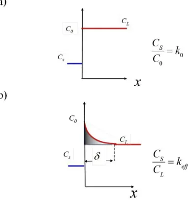
During plane front solidification used to grow single crystals, the concentration of a solute in the solid CS , is different from the concentration in the melt, CL. In equilibrium segregation,

the concentration in the melt is uniform because (a) the freezing rate is low,f→0, and/or, (b) melt is homogenized by perfect mixing. The equilibrium segregation coefficient k0 is,

0 0

/

S

C C k (1)

where C0 =CL [atoms/cm3] is solute concentration at the interface, see Fig. 1a).

During actual crystal growth, a finite freezing rate is used, while mixing is not perfect. Thus, an enriched concentration layer builds up ahead of the interface. Referring to Fig. 1 b), the thickness of the layer is



_{. The effective segregation coefficient is,}

/

S L eff

C C k (2)

The Burton, Prim and Slichter‘s BPS model published in 1953, gives keff as a function of



Fig. 1.a) Equilibrium and b) effective segregation coefficients

textbooks on solidification1. For example Glicksman (2011) states: ―The model, now referred to as BPS theory, captures with astounding simplicity several of the major features to be considered when the melt ahead of the solid–liquid interface is stirred―. Rosenberger (1979) describes the model as a ―hybrid of the stagnant film model, and a full-fledged fluid dynamic boundary layer treatment‖.

During the past sixty years, the shortcomings of the BPS model have been recognized. Several models for keff have been proposed (Wilson 1978; Ostrogorsky and Muller 1992; Yen

and Tiller 1992; Garandet 2008) . Yet, these models give keff is a function of layer thickness



. Here we revisit the film models and compare to the recently proposed model, where keff is a

function of convection coefficient h(Ostrogorsky 2012), or its dimensionless form, /

NuhL D where Nu is Nusselt number , D[cm2/s] is diffusion coefficient and L[cm] is characteristic length.

2. Film-thickness formulations

2.1 keff vs. static film thickness static(BPS model)

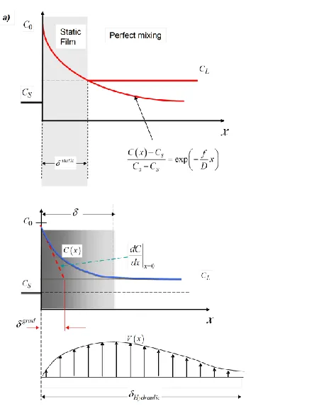
The starting point of the BPS model is the assumption that a stagnant-film exists between the solid-liquid interface and the perfectly mixed region (Fig. 2 a). Within the static film, the concentration profile is exponential, and equal to the steady-state diffusion-controlled profile (Tiller et al. 1953),

 

0

exp

S S

C x C f

x

C C D

 _{ }

 _ _

   (3)

D[cm2/s]is diffusion coefficient, and f[cm/s] is the rate of crystallization. The static-film thickness is introduced by imposing



static



L C  C ,

0

exp static

L S

S

C C f

C C D

 _ _ 

 

   (4)

Here we use superscript ―static‖ to distinguish the static film. Rearranging and using

0 S/ 0

k C C , gives the BPS formula,





_

0

_

0 1 0

static S eff L static C k k

C k k e

f D          (5)

Note that static films do not exist on Earth2. Thus, static _{is a fictitious parameter, and as such it}

can not be calculated (Levich 1961, Wilcox 2004). For small enough values of f cm s



/



, the BPS model makes the unjustifiable assumption,

1/3 1/6 1/ 2

0 1.61

static grad

f D

   



  (6)

where superscript ―grad‖ is used because grad _{is distance between x=0 and the point where}

the gradient

0 /

x

dC dx _ intersects , see Fig. 2 b). Equation (6) was derived by Levich in

(1942) and (1961). It is based on the exact flow solution3. Levich derived the mass flux j from the surface of the impermeable rotating disk to be (see p.69, Levich 1961)





2/3 1/6 1/ 2

0 0.62 0

f L

j   D   C C (7)

where [cm2/s] is kinemetaic viscosity, and [1/s] is disk rotation rate. Levich defined the film thickness as,





0 0

0 /

grad L L

x

C C C C

D

j D dC dx





 

 

 (8)

Substituting eq. (7) into (8) gives eq. (6),





1/3

0 1.61 / /

grad

f D

 _     (9)

Furthermore,





1/3

0 0.5 /

grad

f D Hydraulic

     (10)

0 0.5

grad f

    ₍₁₁₎

2

Static films are presumed to exist in steady-state diffusion-controlled segregation in space laboratories (Witt et. al. 1975)

3 _{von Karman‘s (1921) and Cochran‘s (1934) similarity solution of Navier-Stokes equations for} laminar flow near an infinite rotating disk.

where _Hydraulicand  _{are respectively the actual velocity and concentration boundary layer}

thickness, unrelated to



static

(see Fig. 2b).

2.2 keff vs. dynamic film thickness, grad

Wilson (1978) and Garandet (1993) recognized the shortcomings of the stagnant film formulation, and the exponential concentration profile used in BPS. Wilson and Garandet defined film thickness as Levich, equ. (8), and proceeded to show that the correct formula for

keff is,





_

0

_

0

1 1

grad eff

k k

k

 

   (12)

where _{, is based on gradient thickness,}



3



0

/ exp

grad

f D z Bz dz



  

_

  (13)

whereB0.17f3 3/2 1/2D2. Equations (12) and (13) will be referred to as the Wilson-Garandet’s exact solution.

Wilson(1979) proposed the following approximation,

2/3 1/6 1/ 2 1.61

1

D f

 

   

   

(14)

and determined that it yields less than 0.8 % if 0  0.5. Equation (12) with (14) will be referred to as Wilson‘s approximation-model.

3.Convection coefficient formulation

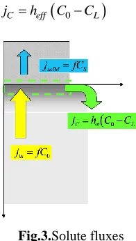
In steady-state, mass conservation requires that all solute released at the crystal-melt interface, is swept away by convection (Ostrogorsky 2012), see Fig. 3,

in solid C

j j j

where the convective mass flux is expressed via the convection coefficient h_eff



cm s/



,



0



C eff L

j h C C (15)

Fig.3.Solute fluxes

The heat transfer analog of equ. (15) is known as the Newton‘s law of cooling. Referring to Fig. 3,



0 S



eff



0 L



f C C h C C

Rearranging and using k₀ CS /C₀, and yields,

 





0

0

1 1

S eff eff

L

ff

C k

k h

f C

k h

 

 

(16)

Comparing eqs. (12) and (16) gives,

/ eff f h

 

3.1

Impermeable Interface

The interface can be considered impermeable for f 0.1h_mix. (Ostrogorsky 2012).

Numerous analytical and empirical correlations for h (i.e. Nu) have been developed for impermeable interfaces (Incropera and DeWitt 1985; Cengel and Ghajar 2010). For forced convection,



1/3



Re ,n

FC

FC L

h L

Nu f Sc

D

  (17)

where Re is Reynolds number and Sc is Schmidt number. n=0.5 and n=0.8 for laminar and turbulent flow respectively. It is interesting to note that Levich did not provide a formula for h, although it is obvious from the flux (7) and the eq. (15),

2/3 1/ 6 1/ 2 0.62

FC

h  D   (18)

The dimensionless form of eq. (18) is,

1/3 /

0.62

FC

h

Nu Sc

D

 

  (19)

where L  / is the characteristic length scale. Equations (18) and (19) are valid only for steady laminar flow, forced convection from impermeable rotating disk (f=0), for Sc .

The general form of the correlations for natural convection is,





n

NC

NC L

h L

Nu f Gr Sc

D

  . (20)

where Gr is Grashof number. n=1/3 and n=1/4 for laminar and turbulent flow respectively. For mixed convection,





1/

/ m m m

mix nix FC NC

Nu h L D Nu Nu

or,

1/m

m m

mix FC NC

h  h h (21)

where m=3 for a vertical surface and m=3.5 for a horizontal surface. hmix is mass transfer

coefficient which accounts for ―mixed convection‖(Incropera and DeWitt 1985; Cengel and Ghajar 2010), and the sign is: + when forced and buoyant convection act in the same direction, or - when forced and buoyant convection act in the opposite direction.

3.2 Permeable interface with uniform or suction

Using the fluid mechanics terminology, the flow velocity perpendicular to the porous interface is ―uniform suction‖ velocity (Schlichting 1968; White 1991). The effect of suction is to stabilize the boundary layers4 by reducing their thickness (Schlichting 1968).

Reducing boundary layer thickness also enhances convection. Since correlations for interfaces with suction are not available, it has been proposed to use an effective convection coefficientdefined as (Ostrogorsky 2012),



_{n n}



1/n eff mix

h  h  f (22)

where n is to be determined from experiments or theory. Combining eqs. (16) and (22) gives,

 









0 0 1/ 1 1 S eff L n n n mix C k k h f C _k h f     

. (23)

Comparing eqs. (12) and (23) gives,





1/n

n n

eff mix

f f

h _{h f}

  

 (24)

3.4 Czochralski growth

In most CZ melts, natural convection and/or turbulence are significant. Since forced and buoyant convection act in the opposite direction, hmix=(hmix

3.5

+f3.5)1/3.5 . The convection coefficients to be used in eq. (21) are (Ostrogorsky 2012):

for laminar flow and 10<Sc<100,







0.373 1/ 4 0.485 / 0.54 / FC NC

h D Sc

h D L Gr Sc

 



  ;

or for turbulent flow,











0.8 0.6

1/3

/ 0.0267 Re

0.15 /

FC r

NC

h D r Sc

h D L Gr Sc



  .

4.Assessment of the models applied to forced laminar convection

For forces laminar convection near a rotating disk, and Sc , the Wilson-Garandet‘s Model, eqs. (12) with (13), provides accurate reference values for keff , because it is based on the

exact solution of the concentration field near the disk. To asses the precision of the models, keff

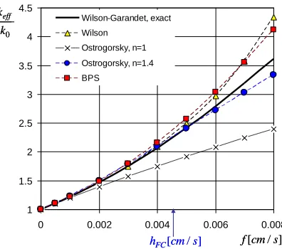
was calculated for the properties and parameters used are for the BPS experiments with Ga-doped Ge: =0.0013 cm2/s , D=2.8x10-5 cm2/s, 60 RMP5, while the range of growth rate is

0<f<0.008 cm/s (=80 μm/s=28.8 cm/hr).

Figure 4 shows keff as a function of the growth rate f, calculated using:

(i) BPS model, eq.(5) with (6), assuming 0

static grad f

  _

(squares)

(ii) Wilson-Garandet‘s exact model eqs. (12) and (13) , where  is obtained by numerical integration (full line).

(ii) Wilson‘s Approximate-model, eqs. (12) and (14) for  (triangles),

(iii) Ostrogorsky‘s model, equ. (23); hmix=hFC = 0.0045 cm/s is calculated using eq. (18). Crosses are for n=1; circles for n=1.4.

Figure 4. verifies the validity of the convection coefficient model, for laminar forced convection in CZ growth. n=1.4 gives a perfect fit for 0<f/hFC<1.3, or f<0.006 cm/s~ 21 cm/hr. n=1 is useful up to ~ 0.001 cm/s=3.6 cm/hr.

Fig. 4.k_eff /k₀ vs. growth rate. Full line: exact Wilson-Garandet‘s model eqs. (12) and (13). Triangles: Wilson‘s model, eqs. (12) and (14). Circles, and crosses are respectively n=1, n=1.4

in eq. (23) . Squares: BPS model.

5. Discussion

The stagnant film concept is unsatisfactory, because their thickness can not be calculated apriori (Levich 1961). In the BPS model, the exponential profile within the stagnant film thickness leads to a great deal of confusion. Assuming static₌

0

grad f

  has no foundation, since static corresponds to the exponential profile, while grad₀

f

  corresponds to the linear profile (Fig. 2).

Fig. 4 reveals that the BPS model is accurate for 1k_eff /k₀2 or f h_FC. In typical CZ system, convection leads to thin solute layers while the f is low. For small   f_fgrad_0 /D, the one term Taylor series expansion, transforms fictitious exponential profile into linear,

1

e  

and turns the BPS formula into eq. (12) or (16). For



static 0, the exponential and linear profiles nearly overlap, Fig. 2). This, Wilson‘s (1979) comment: ―the right answer has been obtained for the wrong reason‖ appears justified.

Kodera‘s (1953) use of the BPS model to determine the diffusion coefficients in Si is problematic. Kodera grew Si crystals at 5, 55 and 200 RPM. Note that at 5 RPM, convection is dominated by buoyancy forces, while at 200 RPM it is likely to be of turbulent. Kodera did not provide the dimensions of the crystals and melts, but according to Ristorcelli and Lumley (1992) even relatively small silicon melts are expected to be turbulent. In turbulent flow,

1 1.5 2 2.5 3 3.5 4 4.5

0 0.002 0.004 0.006 0.008

Wilson-Garandet, exact Wilson Ostrogorsky, n=1 Ostrogorsky, n=1.4 BPS [ / ] f cm s

[ / ]

FC

h cm s

0 eff k k 1 1.5 2 2.5 3 3.5 4 4.5

0 0.002 0.004 0.006 0.008

Wilson-Garandet, exact Wilson Ostrogorsky, n=1 Ostrogorsky, n=1.4 BPS [ / ] f cm s

[ / ]

FC

h cm s

0

eff k

momentum, heat, mass transfer are dominated by eddy-mixing (Muller and Ostrogorsky 1994), while molecular transport weak. In turbulent flow, a concentration gradient C/x induces an apparent mass flux,





apparent D

C

j D

x

 

  

 (25)

where εD is turbulent eddy-diffusivity. Typically, εD>>D. Thus, Kodera‘s high diffusion coefficient for indium, DIn= 6.9x10

4

cm2/s compared to that of boron DB=2.4x10 4

cm2/s may be explained by the presence of eddy-diffusivity, not by high molecular diffusivity. Furthermore, to fit the data, Kodera used viscosity three times higher than the actual. Kodera‘s diffusion coefficients are listed in most handbooks. Diffusion coefficients should not be measured in turbulent melts.

The Wilson-Garandet’s formulation based on the linear profile is consistent, and exact. Its limitations originate in the von Karman‘s/Cochran‘s similarity solution: it is applicable exclusively to laminar flow near a rotating disk, and Sc→∞.

The Wilson’s approximation, (using eq. (14) for ) is precise for 1k_eff /k₀2, or

FC

f h .

The Convection Coefficient Formulation (Ostrogorsky 2012), is based on mass conservation, and as such, equation (16) is exact. For steady laminar flows, the formula

heff=(hmix1.4+f1.4)1/1.4 gives a solid agreement with the exact solution. For impermeable

interfaces, well established correlations for hFC and hNC are available. Thus, Convection

Coefficient Formulation can be applied to a variety of melt-flow conditions, including: (a) turbulent flow; (b) natural convection/mixed convection; (c) finite Sc numbers.

The remaining issue is the lack of correlations for convective coefficients h along interfaces with suction. More data are needed to determine n for turbulent flow with suction.

6. Conclusions

The film-thickness based models are limited by the restrictions carried over from the von Karman‘s/Cochran/ Levich solution. They are valid only for steady laminar flow near a rotating disk.

The recently proposed convection-coefficient formulation (Ostrogorsky 2012), is more general than the models based on Levich‘s film thickness. It is based on mass conservation and as such is exact. It is applicable to turbulent flow, natural and mixed convection, finite Sc numbers. This is a principal advantage considering that (i) most semiconductor melts are turbulent (Ristorcelli and Lumley 1992), and (ii) natural convection on Earth is unavoidable.

For steady laminar flow near a rotating disk, n=1.4 should be used in eq. (23).

Извод

Дебљина слоја и формулација конвективног коефицијента k

eff

A. G. Ostrogorsky

MMAE, Illinois Institute of Technology, Chicago, IL 60616 [email protected]

Резиме

Burton, Prim и Slichter‘s (BPS) модел публикован 1953. год. се сматра најкориснијим моделом за раст кристала и приказан је у већини књига за очвршћавање. Овај модел карактерише коефицијент сегрегације keff као функција константне дебљине филма .

Последњих година се уочавају недостаци BPS модела и предлажу се нови модели који се заснивају на дебљини слоја. У овом раду поново се разматрају модели засновани на дебљини слоја и пореде са недавно предложеним моделом где је коефицијент keff

функција конвективног коефицијента

_h

.

Кључне речи: BPS, сегрегација, конвекција, Czochralski процес

References:

Burton J.A, Prim R.C. , Slichter W.P. (1953) J. Chem. Phys. 21 1991. Burton J.A, Prim R.C. , Slichter W.P. (1953) J.Chem.Phys. 21 1987.

Cengel J.A. and Ghajar A.J. (2010) ―Heat and Mass Transfer‖ 4th Ed., McGraw Hill, New York

Cochran W.G. (1934), Proc. Cambridge Phil. Soc. 30 365. Garandet J.P , (2008) J. Crystal Growth 310 3268– 3273 J.P. Garandet, (1993) J. Crystal Growth 131, 431-438

Glicksman M. E. (2011) ―Principles of Solidification‖ , Springer Verlag,. Hurle D.T.J. and Rudolph P. (2004) J.Crystal Growth 264, 550–564

Incropera F. P. and DeWitt D. P. (1985) ―Introduction to Heat Transfer‖, 2nd ed. Wiley. Kodera H (1963). Jpn. J. Appl. Phys. 2, 212.

Levich V.G. (1942) Acta Physicochem. U. R. S.S. 17, 257

Levich V.G. (1961) Physicochemical Hydrodynamics (Prentice-Hall, Englewood Cliffs, NJ Muller G and Ostrogorsky AG (1994) "Convection in Melt Growth", Chapter 13, Handbook of

Crystal Growth, Vol. 2, Editor: D.T.J. Hurle, North-Holland/Elsevier, pp. 709–819. Ostrogorsky AG (2012) J. Crystal Growth 348, 97-105

Ostrogorsky AG and Muller G (1992) J. Crystal Growth 121, 587–598 Ristorcelli J.R. and Lumley J.L (1992) J. Crystal Growth 116, 447-460.

Welty J.R.,Wicks C.E.,Wilson R.E. (1969) ―Fundamentals of Momentum Heat and Mass Transfer‖, John Wiley and Sons.

White F. (1991), Viscous Fluid Flow (2nd ed.) M. McGraw-Hill, Inc.. Wilcox W.R. (2004) Book Reviews, Cryst. Growth Des. 4, 639, Wilson L.O. (1978) , J. Crystal Growth 44, 247-250

Witt AF, Gatos HC, Lichtensteiger M. , Lavine MC, Hermn CJ (1975), J. Electrochem. Soc. 122-276.