INTRODUCTION
Today, the noise pollution is one of the prin-cipal types of urban natural contamination. What is more, it is responsible for the negative effects that are harmful to the Earth and the personal wel-fare of the people. The increase in noise pollution relies upon numerous elements and in addition, they increase in the urban population and thus the expansion in the number of development ex-ercises and vehicles [Directive EP, 2002]. Noise pollution can be considered as one of the signifi-cant toxins present in urban areas. Its assessment, control, and decrease are among the major natu-ral well-being concerns for specialists [Moham-madi, 2009; Zannin, et al., 2013]. Many research-ers have also reported that road traffic is the most general and prominent noise pollution source in the developing countries [Mocuta, 2012]. Some researchers from different countries also inves-tigated and characterized noise pollution under different types of traffic conditions [Boer, 2007; Stoilova and Stoilove, 1998, Zannin, et al., 2003;
Piccolo, et al., 2205; Zannin, et al., 2006]. The increase in noise pollution is not sustainable be-cause it involves direct, but also cumulative, ad-verse health effects. It also harmfully affects the future generations and has socio-cultural, aes-thetic and economic effects. Noise monitoring under different road and environment condition is one of the best tools to discover the critical lo-cations in residential, commercial and industrial areas [Akhter, et al., 2016]. In order to develop an acoustic model, it is necessary to know as many details as possible [Iliescui, et al., 2015]. The traf-fic noise prediction models are required to assist in the design of highways and roads and some-times, in the evaluation of the existing or planned changes in the traffic noise conditions. Normally, for prediction of the sound pressure levels, the noise levels in terms of Leq are required by most of the sound prediction models [Steele, 2001]. The results from the noise prediction model may further be used for the development of 2D and 3D noise maps [Stoter, et al., 2008]. Noise map-ping is the graphic representation of the sound
Accepted: 2020.04.04 Available online: 2020.04.17
Volume 21, Issue 4, May 2020, pages 82–93 https://doi.org/10.12911/22998993/119804
Noise Monitoring, Mapping, and Modelling Studies – A Review
Pervez Alam
1*,
Kafeel Ahmad
1, Shakil S. Afsar
1, Nasim Akhtar
21 Department of Civil Engineering, Jamia Millia Islamia, 110025, New Delhi, India
2 CSIR, CRRI, Mathura Road, New Delhi, India
* Corresponding author’s e-mail: pervezjmi@gmail.com
ABSTRACT
This paper reviews the literature on noise monitoring, noise mapping and noise modeling studies carried out in
different countries by many researchers. The article reveals the current status of the noise-related studies and noise mapping studies. It was discovered that 90% of the noise monitoring studies were focused on the traffic noise, while
the remaining 10% focused on the residential, commercial and industrial areas. Sometimes, there may be a necessity to analyze the sound pressure levels all over the place, or around a particular piece of land and machinery of indus-try. Researchers have used the noise monitoring data for the development of 2D and 3D noise maps which gives a clear picture of the noise level around the source of noise in X, Y, and Z direction. For taking a decision regarding the
noise level for any development project, predicting the noise level is always necessary. The traffic noise models are
generally used for the purpose of prediction. Early models are based on constant vehicle speed, later some models
predicted the noise level for interrupting the traffic flow. For instance, the Stop and Go model can be used for the prediction of the noise level in an interrupted flow. Four such models were reviewed and compared in this article.
level distribution existing in a given region and environmental condition, for a defined period of time. Noise mapping is broadly divided into two categories i.e., 2D and 3D. The 2D mapping has been extensively and successfully used for envi-ronmental impact studies like Air pollution, Soil pollution and Noise in the existing environment. Noise monitoring, mapping, and modeling stud-ies are interrelated. The results of noise monitor-ing can be used for the prediction of the sound pressure level employing different prediction models; the predicted results may further be used for the development of noise maps.
NOISE MONITORING STUDIES
IN DEVELOPING COUNTRIES
Significant negative effects on the children’s blood pressure and mental health due to noise pollution have been found. Some studies show that the people who are exposed to high street traffic noise levels often suffer from hyperten-sion [Chang, et al., 2011]. The noise monitoring studies are especially needed for monitoring the sound levels and appropriate reduction measures can be implemented to control the noise pollution [Garg, et al., 2017]. Studies on monitoring and applying noise abatement measures to ambient noise and controlling them have been conducted in various parts of the world. The advancement of developing countries is accompanied by in-dustrialization. We see not only a higher level of noise in industry and traffic, but also a concentra-tion of populaconcentra-tion, on the one hand, and a higher construction of high rise buildings on the other [Barrekette, 1973]. The noise monitoring studies of 22 developing countries and 25 cities for two decades were reviewed to demonstrate the current state of the investigation on the acoustic pollution in developing countries and the gaps in the stud-ies. Table 1 shows the maximum, equivalent and minimum noise level of developing countries. A noise monitoring study was performed by [Chow-dhury, et al., 2010] at Dhaka city of Bangladesh. The monitoring results show a maximum noise level of 87 dB (A) and Leq of 82 dB (A) is enough to create discomfort for the people living in the nearby areas. A study conducted in China, Brazil, Egypt, and Iraq [Bengang, et al., 2002; Henrique, et al., 2002; Zekry and Ghatass, 2009] revealed that the equivalent noise level at the study area of these countries remains in between 75.2 dB to
75.35 dB, which is also higher than the prescribed standard of these all locations. The noise study at Columbia [Danie, et al., 2014] and Poland [41] only shows the Leq noise level within the pre-scribed standard. However, noise monitoring in Nigeria [Avwiri, and Nte., 2003] and the Philip-pines [Vergel et. al., 2004] shows the maximum noise level among all 22 developing countries i.e., 81.4 and 84.3 dB, respectively. The noise monitoring was carried out in three states of India by Rajiv B. Hunashala, Yogesh B. Patil, Pervez Alam et al., and Ambika N. Joshi et al. The re-sults show that the equivalent noise level remains maximum at Mumbai [72.0 dB] followed by Delhi [70.2 dB] and Kolhapur [65.3]. Thus, the noise level of these three cities of India remains higher than the prescribed standard of Central pollution Control Board (CPCB). Furthermore, it has been found that most of the study areas of the selected developing countries have been exposed to the noise levels higher than the prescribed stan-dard of the competent authority in the respective countries.
NOISE MAPPING
OF DEVELOPING COUNTRIES
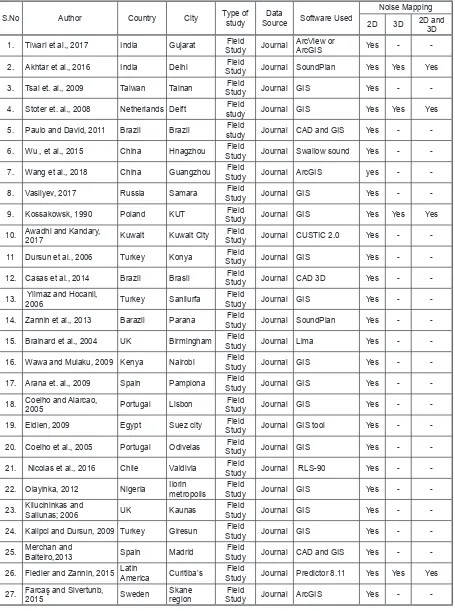
cities for around two decades to demonstrate the current state of the noise mapping studies in de-veloping countries and the gaps in the studies. Table 2 shows the assessment of 2D and 3D noise mapping of developing countries. In India [Ti-wari et al., 2017; Akhtar et al., 2016] performed the 2D and 3D noise mapping for Gujarat and Delhi, using ArcView and soundPlan software,
respectively. Using 2D noise mapping in Guja-rat, Tiwari et al. were able to establish a critical location where remedial measures are required to reduce the adverse effect of noise on human beings. Furthermore, [Nasim Akhtar et al., 2016] has also developed 2D as well as 3D noise maps for selected locations of Delhi. Their study shows the importance of a 3D noise map, as using 3D
Table 1. Maximum, equivalent and minimum noise level of developing countries
S.No Author Country City Type of study SourceData measurementNoise Noise levels (dB A) Lmax Leq Lmin 1. Chowdhury et,al., 2010 Bangladesh Dhaka SurveyField Journal Yes 87 82.0 53
2. Bengang et.al., 2002 China Beijing SurveyField Journal Yes 87.3 75.2
-3. Zannin, 2002 Brazil Curitiba SurveyField Journal Yes - 75.6
-4 Ghatass, 2009 Egypt Alexandria SurveyField Journal Yes 47.7 75.6 98.7
5. Essandoh and Frederick, 2011 Ghana Cape Coast SurveyField Journal Yes 87.3 73.5 51.1
6. Galindo, et al., 2017 Colombia Santa Marta SurveyField Journal Yes 76.04 64.0 54.8
7. Daniel et al., 2014 Colombia Bagota SurveyField Journal Yes 65.3 56.5 45.7
8. Mesfin, et.al., 2018 Ethiopia Dire-Dawa City surveyField Journal Yes 68.08 - 52.26
9. Abankwa, et al., 2017 Ghana Kumasi surveyField Journal Yes 83.5 72.6 66.8
10. Hunashala and Patil, 2012 India Kolhapur SurveyField Journal Yes 73.7 65.3
-11. Akhtar et al., 2016 India Delhi SurveyField Journal Yes 79.3 70.2 60.2`
12 Joshi, et.al., 2015 India Mumbai SurveyField Journal Yes 80.6 72.0 64.5
13. Sondakh et. al., 2014 Indonesia Ratulangi Manado SurveyField Journal Yes 87.4 71.6 49.2
14. Biglari et al., 2016 Iran Tehran surveyField Journal Yes 102.57 75.3 66.7
Rauf et al., 2015 Iraq Sulaimani surveyField Journal Yes 75.5 65.3 55.4 Awadhi and kandari,
2017 Kuwait Kuwait City SurveyField Journal Yes 82.0 80.0 70.5 Aziz et al., 2012 Iraq Erbil SurveyField Journal Yes 85.0 75.2 69.1
Fernandez et. al., 2013 Maxico Maxico City SurveyField Journal Yes 80.1 77.2 58.1
Avwiri, and Nte., 2003 Nigeria Nigeria Delta SurveyField Journal Yes 93.2 81.4 68.3
Vergel et. al., 2004 Philippine Quezon City SurveyField Journal Yes 95.6 84.3 70.1
Vasilyev et. al., 2017 Russai Samara SurveyField Journal Yes 80.1 65.3 52.0
Zytoon, 2016 Saudi Arabia Jeddah SurveyField Journal Yes 70.1 62.3 50.5
Vasilyev, 2017 Russia Samara SurveyField Journal Yes 65.6 59.8 46.2
Çoban et al., 2018 Turkey Turkey City surveyField Journal Yes 76.2 61.3 52.5 Szopinska and Rącka,
mapping enables to locate the effects of noise pol-lution in X, Y and Z direction on any residential building or setup. Most of the researchers used GIS as a tool for development of 2D noise map in different countries like Taiwan, Netherlands, Russia, Poland, Turkey, Kenya, Spain, Nigeria, Portugal and Egypt. In some countries, research-ers used other tools for the development of noise maps; for instance, Nasim Akhter et al. (in India), and Zannin et al. (In Brazil) used soundPlan for the development of 2D and 3D mapping. In Chi-na, [Wu, et al., 2018] used Swallow sound for the development of a 2D noise map for the selected locations. In Latin America [Fiedler and Zannin, 2015], used Predictor 8.11 for the development of 2D and 3D noise mapping for the selected loca-tion of the Curitiba city. CAD 3D software has also been used in two countries i.e., in Spain and Brazil, in Madrid and Brasilia, respectively, for the 2d noise mapping only. Most of the research-ers have developed 2D noise maps only for the selected locations of different countries such as [Kartikey Tiwari et al., 2017] for India, [Tsai et al., 2009] for Taiwan, [Paulo and David, 2011] for Brazil, [Wu, 2015] for China, [Vasilyev, 2017] for Russia, [Awadhi and Kandary, 2017] for Kuwait, [Dursun et. al., 2006] for Turkey, Brainard et al., 2004 for United Kingdom, [Wawa and Mulaku, 2009] for Kenya, [Arana et al. 2009] for Spain, [Coelho and Alarcao, 2005] for Portugal, [Eldien, 2009] for Egypt, [Nicolas et al., 2016] for Chile, [Olayinka, 2012] for Nigeria, and [Farcaş and Sivertunb, 2015] for Sweden. Few researchers have developed 3D noise maps for a selected lo-cation of some countries, such as [Nasim Akhtar et al., 2016] for India, [Stoter et al., 2008] for the Netherlands, [Kossakowski, 1990] for Poland, [Fiedler and Zannin, 2015] for Latin America. As per the above literature review of 2D and 3D noise mapping, it has been established that the 2D noise maps have been developed by most of the researchers for their respective developing coun-tries to find out the distribution of noise along a central line of a road or along the periphery of an industry. However, the literature survey also shows that the 3D noise gives a clear picture of the noise distribution in all three directions X, Y, and Z. In one of the studies of India, 3D noise maps have been developed by [Akhtar, et al., 2016] for the selected location of Delhi which gives clear picture of noise distribution in all three directions and also provides a number of the people affected in a particular residential building. Thus, from the
review of noise mapping it can be concluded that the 2D noise mapping is an effective way to show the noise level distribution along with any source of noise in X and Y direction only. The 3D noise mapping is more effective than 2D in the residen-tial areas, as it can also provide noise exposure level in the Z direction and also gives a number of people affected in high rise residential buildings. The review also shows that very few research works has been performed in the field of 3D noise mapping. On the other hand, 2D noise mapping has been used extensively by researchers.
NOISE PREDICTION MODELS STUDY
Noise prediction is one of the essential tools for decision-makers to reduce the adverse effect of noise and their control. The prediction mod-els are generally used by three major sections of society.
1. Acoustic Engineers: Acoustical engineers are generally worried about the plan, investigation, and control of sound.
2. Acoustic specialist: They are generally part of the team to prepare an environmental impact assessment report.
3. Decision maker: Prediction models are gener-ally used by decision-makers to identify the distribution of noise in the upcoming days.
in 2001, but some of them have been revised between 2007–2013 and updated by [Garg and Maji, 2014] in 2014. Now, they have been around for six years; thus, it is imperative to update the
comparison done by Garg and Maji again. The present study reviews the implication and strat-egies of the recently developed models such as CoRTN, Start and Stop, FHWA, etc.
Table 2. Assessment of 2D and 3D noise mapping of developing countries
S.No Author Country City Type of study SourceData Software Used Noise Mapping 2D 3D 2D and 3D
1. Tiwari et al., 2017 India Gujarat StudyField Journal ArcView or ArcGIS Yes -
-2. Akhtar et al., 2016 India Delhi StudyField Journal SoundPlan Yes Yes Yes
3. Tsai et. al., 2009 Taiwan Tainan StudyField Journal GIS Yes -
-4. Stoter et. al., 2008 Netherlands Delft studyField Journal GIS Yes Yes Yes
5. Paulo and David, 2011 Brazil Brazil studyField Journal CAD and GIS Yes -
-6. Wu , et al., 2015 China Hnagzhou StudyField Journal Swallow sound Yes -
-7. Wang et al., 2018 China Guangzhou StudyField Journal ArcGIS yes -
-8. Vasilyev, 2017 Russia Samara StudyField Journal GIS Yes -
-9. Kossakowsk, 1990 Poland KUT StudyField Journal GIS Yes Yes Yes
10. Awadhi and Kandary, 2017 Kuwait Kuwait City StudyField Journal CUSTIC 2.0 Yes -
-11 Dursun et al., 2006 Turkey Konya StudyField Journal GIS Yes -
-12. Casas et al., 2014 Brazil Brasil StudyField Journal CAD 3D Yes -
-13. Yilmaz and Hocanli, 2006 Turkey Sanliurfa StudyField Journal GIS Yes -
-14. Zannin et al., 2013 Barazil Parana StudyField Journal SoundPlan Yes -
-15. Brainard et al., 2004 UK Birmingham StudyField Journal Lima Yes -
-16. Wawa and Mulaku, 2009 Kenya Nairobi StudyField Journal GIS Yes -
-17. Arana et. al., 2009 Spain Pamplona StudyField Journal GIS Yes -
-18. Coelho and Alarcao, 2005 Portugal Lisbon StudyField Journal GIS Yes -
-19. Eldien, 2009 Egypt Suez city StudyField Journal GIS tool Yes -
-20. Coelho et al., 2005 Portugal Odivelas StudyField Journal GIS Yes -
-21. Nicolas et al., 2016 Chile Valdivia StudyField Journal RLS-90 Yes -
-22. Olayinka, 2012 Nigeria Ilorin metropolis StudyField Journal GIS Yes -
-23. Kliucininkas and Saliunas; 2006 UK Kaunas StudyField Journal GIS Yes -
-24. Kalipci and Dursun, 2009 Turkey Giresun StudyField Journal GIS Yes -
-25. Merchan and Balteiro,2013 Spain Madrid StudyField Journal CAD and GIS Yes -
-26. Fiedler and Zannin, 2015 Latin America Curitiba’s StudyField Journal Predictor 8.11 Yes Yes Yes
-FHWA Traffic Noise Model Version 3.0 (2016)
Federal Highway Administration (FHWA) Traffic Noise Prediction Model [Anon, 1978] was developed for the United States of America (USA) Department of Transportation Federal Highway administration by Barry and Reagan (1976); they received help from preceding Na-tional Cooperative Highway Research Program (NCHRP) [Anon, 1976]. The prediction noise model was published as a Report No. FHWA-RD-77–108 which included calculation and pro-grammable program. The reference noise level is the maximum noise level of the vehicle, emitted by the vehicle passed at a distance of 15 m. In the FHWA model, Leq (Near) and Leq (Far) were calculated and the average of far and near were taken into consideration for noise average Leq noise level.
Leq (near)=10log (∑alli 10Leq (hi) (near)/10) (1)
where Leq (near)= Noise level of all classes of ve-hicles from the near side of the road
Leq (hi) (near)= The noise level of vehicle class-I from near side of the road
Leq (far): 10log ∑alli 10Leq (hi) (far)/10) (2)
where: Leq (far) = Noise level of all classes of ve-hicles from the far side of the highway
Leq(hi) (far)= Noise level of vehicle class I from the far side of the highway
Leq(hourly)= ELi + A(traffic) + Ad + As (3) where: A (traffic) = Correction for traffic flow
Ad = Correction for distance between the roadway and receiver
As = Correction for all shielding and ground effects between the roadway and the receiver.
Assumption for noise prediction (FHWA)
The following are the major assumption for the prediction of the noise level by FHWA
1. The vehicles will be represented as an acoustic source .
2. Noise emission levels will be assumed as group noise source such as (Bus, medium and heavy trucks) are normally distributed.
3. Noise propagation losses will be adequately represented by the effect of distance.
Input Parameters required for prediction of noise level (FHWA)
For validating the FHWA model, traffic noise monitoring, the characteristics of traffic, includ-ing its composition and volume of traffic on the road, are required. For the FHWA model, traffic composition is normally divided into each type of vehicle such as medium truck, heavy truck and passenger car. The light vehicles included per-sonal cars, local taxis, vans, and motorized two-wheelers, while trucks and buses are included as the heavy vehicles.
RLS-90 model
RLS90 is an efficient model, able to determine the noise pollution level of road traffic and, in current days, is the main appropriate calculation method used in Germany. It is a German national model for the prediction of road traffic noise and parking noise. It is made up of two different mod-els; the first corresponds to the determination of noise level emission (Lme) at a distance of 25 m from the center of the road and 4 m above the ground level. Lme is determined by taking into consideration traffic such as the speed of the ve-hicle, distribution of the veve-hicle, road surface condition. The sound pressure level for a street:
LT = Lm + K (4)
where: Lm = mean A-weighted noise level
K = Addition for increase in noise due to effect of traffic signal controlled intersec-tions and other intersecintersec-tions
Lme = L25 + Cs + Crs+ Cg + Cr (5) where: L25 = Standardized noise level for assump-tion of a speed amounting to 100 km/h for cars and 80 km/h for trucks.
Cs = Speed correction
Crs = Road surface correction
Cg = Gradient correction
Cr= Multiple reflection correction
L25 = 37.5+10×log10 [M× (1+0.082×P)] (6) where: M = Number of vehicles (h-1)
P = tracks exceeding 2800 kg (%)
addition of all the contributions carried out by the sources taking into account the length of the road, the reduction of noise due to the distance, air absorption, and sound propagation due to the temperature gradient.
Assumption for noise prediction (RLS-90)
The following are the major assumption for the prediction of noise level by the RLS-90 model 1. The day and night time has been assumed as 6
AM to 10 PM and 10 PM to 6 AM, respectively. 2. It will take into account the major features
which influence the noise propagation, such as obstacles, vegetation, absorption, reflections and diffraction [Quartieri et al., 2012 ].
3. Parking spots and the number of vehicles in parking spots will be considered for noise prediction.
Input Parameters required for noise prediction (RLS-90)
Prediction of the noise level by RLS- 90 re-quired some input parameters such as the aver-age hourly flow of traffic, separated two-wheel-ers, light and heavy motor vehicles, the aver-age speed for each group of traffic, road dimen-sion, the geometry of road and road type and any natural and artificial obstacles. This model considers the fundamental highlights which impact the propagation of noise, for example, obstacles, vegetation, reflections, and diffrac-tion. Specifically, it makes checking the noise decrease created by obstacles conceivable and likewise considers the reflections delivered by the screens.
Stop and Go model
Pamanikabud and Tharasawatpipat [1999] of the Urban Transport Department in 1997 de-veloped the Stop and Go model for the central part of Bangkok. The model gives emphasis on formulating an empirical model of the intermit-tent flow of traffic in Bangkok using two ana-lytical approaches. The first is the single model analysis and the second is the separate lane analysis or dual model analysis. Traffic noises due to interrupted or stop and go flow of traf-fic situation on urban roads create considerably diverse noise
Volume of traffic =
= (AU) +1.04(LT) + 1 1.12(MT+TT) + + 1.14(HT) + 1.09(MC+BU + MB) (7) where: MC = Motorcycles
MT = Medium truck
BU = Bus
TT = Tuk-Tuk
MB = Minibus
The single Stop and Go model approach has been firstly applied to build a single stop and go traffic flow, noise model. This model can be used to both sides of an urban roadway. The Leq by Stop and Go single-lane model can be predicted by:
Leq = 71.05 + 0.10Sn + 0.95 Log Vn + + 0.04 Sf + 0.015 Log Vf – 0.111Dg (8) where: Dg – Geometric mean of road section
(m); = (Df x Dn)
In a separate lane model, the Leq noise level for acceleration and deceleration lane are taken into consideration and the average of both lanes remains the actual Leq level. The equation men-tioned below is generally used for the determina-tion of Leq by a separate lane model.
Acceleration lane Stop and Go separate lane model
Leq = 56.91 + 0.09Sn(a) + 5.22 Log Vn(a) + + 0.04Sf (a) + 0.02 Log V (a) – 0.006D(a)
Deceleration lane Stop and Go separate lane model
Leq = 71.12 + 0.07Sn(b) + 0.42 Log Vn(b) + + 0.08Sf (b) + 0.44 Log V (b) – 0.061D(b)
Assumption for noise prediction (Stop and Go Model)
For the prediction of noise characteristics for interrupting traffic flow, the Stop and Go model is used. This model is based on the following assumption.
1. Two modes of vehicles motion
a) Cruising with a steady uniform speed of traffic b) Stopping of traffic
2. The road is a straight, good surface condition, no variation
3. No noise barrier between the observer and the noise source
4. Traffic noise is measured in equivalent noise level (Leq)
Input Parameters required for prediction of noise (Stop and Go Model)
Several parameters are required while pre-dicting noise using the stop and go model. The parameters considered are vehicle volume classi-fied into the different vehicle types appearing on the both sides of the road, average spot speed of vehicles in the traffic stream and roadway width.
CoRTN Model
The noise prediction model CoRTN has been developed by Delany, Harland, Hood, and Scho-les for the United Kingdom (UK) Department of Environmental Engineering [Steele, 2001]. It is generally used as assistance for the design of the road, and also for the prediction of noise level around a noise source. CoRTN assumes a line source and constant speed of traffic, and in the UK it is the only tool for the classification of environmental impact due to the road traffic. Cal-culation of Road Traffic Noise (CoRTN) [Anon, 1975] has been replaced by a handier, Predicting Road Traffic Noise (PRTN) which also followed [Delany et. al., 1976] rationale for the proce-dure. The noise level (predicted or measured) is expressed in terms of L10 (hourly) dB (A) and L10 (18-hour) dB (A): 6:00 to 24:00 hrs. If traffic data has been available hourly, then CoRTN can be used to produce the hourly values of L(A)10 which can then be converted to Leq (A) hourly values. However, for the non-motorway roads when hourly traffic flows are below 200 vehicles per hour during the period 24:00 to 06:00 hours, the following should be used:
Leq(A), hourly = 0.57*L10(A),1h + 24.46 dB For motorways Leq may be calculated using the formula below:
L(Day) = 0.98 X L10,18h + 0.090 dB L(Evening) = 0.89 X L10,18h + 5.080 dB L(Night) = 0.87 X L10,18h + 4.240 dB L(Den) = 0.90 X L10,18h + 9.690 dB
For Non motorways the Leq may be calcu-lated using below mention formula
L(Day) = 0.95 X L10,18h +1.44 dB L(Evening) = 0.97 X L10,18h -2.87 dB L(Night) = 0.90 X L10,18h -3.77 dB L(Den) = 0.92 X L10,18h +4.20 dB
Assumption for noise prediction (CoRTN)
The following parameters have been assumed during noise level prediction.
1. The source height should be 0.5 m above the carriage level.
2. Source distance should be 3.5 m from the near side carriageway edge
3. Noise has been estimated at 1 meter in front of the most exposed part of an external window or door.
4. Meteorological conditions are not taken into consideration.
5. No background noise is taken into consideration.
Input Parameters required for noise prediction (CoRTN)
For validating the CoRTN model, traffic noise monitoring, characteristics of traffic including its composition, the volume of traffic, and vehicle speed on the road have been recorded. In the pro-cess of validation, the CoRTN model and traffic composition are normally divided into the light and heavy vehicles. For this study, the light vehi-cles included personal cars, local taxis, vans, and motorized two-wheelers, while trucks and buses are included as the heavy vehicles.
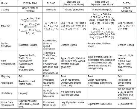
COMPARISON OF MODELS
A comparison of different aspects of princi-pal traffic noise prediction models was shown in Table 3. The main aspects of FHWA-TNM, RLS-90, Stop and Go (Single Lane Model) and Stop and Go (Separate Lane Model) were discussed in the table. Only the Stop and Go model is pre-dicting noise level for interrupting traffic flow. In turn, all remaining models are designed to predict the noise level for uninterrupted traffic flow. In India, the traffic flow is usually interrupted. Thus, the traffic noise model able to predict the noise level in such a complex scenario is still pending to design.
CONCLUSION
1. 90% noise monitoring studies focused on the traffic noise, the remaining 10% focused on the residential, commercial and industrial areas. 2. The 2D noise maps were developed by 95% of
researchers only 5% developed 2D as well as 3D noise maps.
3. Most of the noise prediction models use uni-form traffic flow for the prediction of noise levels, only a few predict the noise levels for uniform as well as interrupted flow.
4. On the basis of the above-mentioned literature survey, it has also been concluded that the noise monitoring has not been carried out in differ-ent seasons and 24 X 7 and the 3D noise maps have not been developed for the assessment of noise level. However, the 2D noise maps are readily developed for noise assessment.
REFERENCES
1. Directive 2002/49/EC of the European Parliament
and of the Council of 25 June 2002 relating to the
assessment and management of environmental noise
(END). Brussels, the European Parliament and the
Council of the European Union, 2002.
2. Mohammadi, 2009. An Investigation of
Commu-nity Respond to Urban Traffic Noise. J Environment Health Science, 2, 137 .
3. Zannin, P.H.T., Engel, M.S., Fiedler, P.E.K., Bunn,
F., 2013. Characterization of Environmental Noise
Based on Noise Measurements, Noise Mapping and
Interviews: a Case Study at a University Campus in
Brazil. Cities, 31, 317.
4. Mocuta, G.E., 2012. Noise Pollution Emitted as a Consequence of the Urban Transport Development. J Environ Prot Ecol, 13 (2A), 852.
5. Eelco, L.C., Boer, D., Schroten, A., 2007. Traffic
Noise Reduction in Europe. CE Delft.
6. Stoilova, K., Stoilov, T., 1998. Traffic Noise and Traffic Light Control. Transportation Research Part D: Trans Environ, 3 (6), 399.
7. Zannin, P. H. T., Calixto, A., Diniz, F. B., Ferreira,
J. A. C., 2003. A Survey of Urban Noise Annoyance
in a Large Brazilian City: the Importance of a Sub
-jective Analysis in Conjunction with an Ob-jective
Table 3. Comparison of noise prediction models
Model FHWA- TNM RLS-90 (Single Lane Model)Stop and Go (Separate Lane Model)Stop and Go CoRTN
Country United State of America Germany Thailand (Bangkok) Thailand (Bangkok) KingdomeUnited
Equation
Leq (near)=10log (∑alli 10Leq (hi) (near)/10)
Leq (far): 10log ∑alli 10Leq (hi) (far)/10)
Leq(hourly)= ELi + A(traffic) + Ad + As
LT = Lm + K Lme = L25 + Cs + Crs+ Cg + Cr
Leq = 71.05 + 0.10Sn + 0.95 Log Vn + 0.04 Sf + 0.015 Log Vf – 0.111Dg
Leq(Acc) = 56.91 + 0.09Sn(a) + 5.22 Log Vn(a) + 0.04Sf (a) + 0.02
Log V (a) – 0.006D (a)
Leq(dec) = 71.12 + 0.07Sn(b) + 0.42 Log Vn(b) + 0.08Sf (b) + 0.44
Log V (b) – 0.061D (b)
Leq(A), hourly = 0.57*L10(A),1h + 24.46 dB
Traffic
Condition Constant, Grades
Acceleration, Uniform speed, intermittent
Uniform Speed Acceleration, Uniform speed, Uniform Speed
Data Requirement
Speed of Traffic, Traffic Flow, Environment Condition and Local characteristics Traffic type, Traffic Flow,, Road data, and Environment Condition and Local characteristics
Type of traffic, Detail of interrupted flow, speed of traffic and road geometry
Type of traffic, Detail of interrupted flow, speed of traffic(Acceleration and deceleration lane) and road geometry
Heavy to Light vehicle Ration, Low, speed, road and environs data.
Mapping Grid Point Point Point Grid
Application Prediction road Traffic noise, Prediction road traffic noise
Urban road traffic, uninterrupted traffic flows (Leq)
Urban road traffic, interrupted traffic flows (Leq)
Prediction of Single traffic noise
Limitations Leq only No local characteristics take cares.
Not take care traffic flow of both lanes
On the basis of L10 Leq is being determine that is obsolete Noise Data
requirement
Equivalent Noise Level and L10 noise level
Equivalent
Analysis. Environ. Impact Asses, 23 (2), 245.
8. Piccolo, A., Plutino, D., Cannistraro, G., 2005, Eval -uation and Analysis of the Environmental Noise of
Messina, Italy. Appl Acoust, 66, 447.
9. Zannin, P.H.T., Ferreira, A.M.C., Szeremetta, B.,
2006, Evaluation of Noise Pollution in Urban Parks. Environ Mon Asses, 118, 423.
10. Akhtar, N., Ahmad, K., and Alam P., 2016, Noise
Monitoring and Mapping for Some Pre-selected Lo-cations of New Delhi, India, Fluctuation and Noise Letters Vol. 15, No. 2.
11. Iliescu, M., Cadar, Y., Beca, M., 2015. Monitoring
Noise Pollution in Urban Area Through SUNET
System, Bulletin USAMV series Agriculture 72(1).
12. Steele, C., (2001), A critical review of some traf
-fic noise prediction models, Applied Acoustics 62, 271–287.
13. J.E. Stoter, H. de Kluijver, V. Kurakula: 3D noise
mapping in urban areas, International Journal of
Geographical Information Science Vol. 22, No. 8,907–924, 2008.
14. Chang T.Y., Liu C.S., Bao B.Y., Li S.F., Chen T.I., Lin Y.J. , Characterization of road traffic noise exposure
and prevalence of hypertension in Central Taiwan,
Science Total Environment, 409, 1053–1057, 2011.
15. Naveen Garg, A.K. Sinha, M. Dahiya, V. Gandhi R.M. Bhardwaj, A.B. Akolkar; Evaluation and
Analysis of Environmental Noise Pollution in Seven Major Cities of India, Archives of Acoustics, Vol.
42, No. 2, pp. 175–188, 2017.
16. E. S. Barrekette, Pollution Springer Science Busi
-ness Media New York 1973.
17. Sanjib Chandra Chowdhury, M. Mahbubur
Raz-zaque, and Md. Maksud Helali; Assessment of Noise Pollution In Dhaka City; 17th international congress of sound and vibration, ICSV17, Cairo, Egypt, 18–22 July 2010.
18. Bengang Li, Shu Tao, R.W. Dawson; Evaluation and analysis of traffic noise from the main urban roads in Beijing; Applied Acoustics 63, 1137–1142, 2002.
19. Paulo Henrique Trombetta Zannin, Fabiano Belisa
-rio Diniz, Wiliam Alves Barbosa; Environmental noise pollution in the city of Curitiba, Brazil; Ap
-plied Acoustics 63 351–358, 2002.
20. Zekry F. Ghatass; Assessment and Analysis of Traf
-fic Noise Pollution in Alexandria City, Egypt; World Applied Sciences Journal 6 (3): 433–441, 2009.
21. Paul K. Essandoh and Frederick Ato Armah; De -termination of Ambient Noise Levels in the Main
Commercial Area of Cape Coast, Ghana;
Research Journal of Environmental and Earth
Sci-ences 3(6): 637–644, 2011.
22. Angélica Patricia Garrido Galindo, Yiniva Ca -margo Caicedo, Andres M Vélez-Pereira; Noise level in a neonatal intensive care unit in Santa
Marta – Colombia; Colombia Médica – Vol. 48, 2017.
23. Paez, Danie; Thirouin, Maïté; Behrentz, Eduardo;
Pacheco, José; Perry, Anthony; Where Are We out?
Spatial Analysis Of Noise Pollution In Bogota; con
-ference_proceedings/Inter Noise 2014.
24. Kinfe Mesfin*, Abdrie Seid Hasen and Mohamed Birhanu; Determination of Noise Pollution Level in
Dire-Dawa City, Ethiopia; Int J Environ Sci Nat Res
8(2): IJESNR.MS.ID.555733, 2018.
25. Abankwa E.O., Agyei-Agyemang A., Tawiah P.O;
Impact of Noise in the Industry and Commercial
ar-eas in Ghana: Case Study of the Kumasi metropolis;
Int. Journal of Engineering Research and
Applica-tion; Vol. 7, Issue 7,, pp.11–19, July 2017
26. Rajiv B. Hunashal, Yogesh B. Patil, 2012. Assess
-ment of noise pollution indices in the city of Kol
-hapur, India; Procedia – Social and Behavioral Sci
-ences 37, 448–457.
27. Nasim Akhtar, Kafeel Ahmad and Pervez Alam;
Noise Monitoring and Mapping for Some Pre-se-lected Locations of New Delhi, India; Fluctuation
and Noise Letters, 15(2), 2016.
28. Ambika N. Josh, Nitesh C. Joshi, Dr. Payal P. Rane;
Noise Mapping in Mumbai City, India; IJISET; 2(3),
2015.
29. Daniel Sondakh1, Maryunani, Soemarno , Budi
Setiawan; Analysis of Noise Pollution on Airport
Environment (Case study of International Airport of Sam Ratulangi Manado, Indonesia); International Journal of Engineering Inventions; 4(2), 2014.
30. Hamed Biglari, Mehdi Saeidi, Mohsen Poursa
-deghiyan, Hooshmand Sharafi, Mohammad Reza
Narooie,Vali Alipour, Somayeh Rahdar, Razieh
Khaksefidi, Amin Zarei, Morteza Ahamadabadi1; A Study On Noise Pollution In The City Of Tehran,
Iran; International Journal of Pharmacy & Technol-ogy; Vol., 3, 2016.
31. Kani M Rauf, Hussein Hossieni, Saro S Ahmad,
Sarkhel Jamal and Aras Hussien; Comparison of the Noise Pollution in Sulaimani City between the Years
2009 and 2014;Pollution effects and control;Volume
3, Issue 1, 2015.
32. jasem M. Al-Awadhi, Dhary S. AlKandary; Map
-ping and Validation of Noise Level in Kuwait City;
Transactions on Science and Technology Vol. 4, No.
1, 38–47, 2017.
33. Shuokr Qarani Aziz Lulusi, Faridah A.H. Asaari,
Nor Azam Ramli Hamidi, Abdul Aziz Amin Mojiri
and Muhammad Umar; Assessment of Traffic Noise Pollution in Bukit Mertajam, Malaysia and Erbil City, Iraq; Caspian Journal of Applied Sciences Re
-search, 1(3), pp. 1–11, 2012.
on Environment, Energy, Ecosystems and Develop-ment 2013.
35. G.O. Avwiri, F. Nte; Environmental sound quality of some selected flow Stations in the Niger delta of
Nigeria; Journal of Applied Sciences and
Environ-mental Management Vol. 7(2) 2003, 75–77
36. Karl N. Vergel, Frielly T. Cacho and Cheryl Lyne E. Capiz; A Study on Roadside Noise Generated
by Tricycles; Philippine Engineering Journal, 2004;
25(2), 1–22.
37. Andrey V. Vasilyev, 2017. New methods and ap -proaches to acoustic monitoring and noise mapping of urban territories and experience of it approbation in conditions of Samara region of Russia; Procedia
Engineering 176, 669–674.
38. Mohamed A. Zytoon; Opportunities for Environ -mental Noise Mapping in Saudi Arabia: A Case of
Traffic Noise Annoyance in an Urban Area in Jed -dah City; Int. J. Environ. Res. Public Health 2016, 13, 496.
39. Nilgün Akbulut Çoban, Cengiz Dalkılıç, Sezer Kaya, Mevlüt Türkmenoğlu, and Mustafa Çoban;
Smart Solutions for Recreational Noise Pollution
in Turkey; Noise Mapp. 2018; 5:21–32.
40. Kinga Szopińska and Izabela Rącka; Assessment
of the Sound Environment and Prices of
Noise-Sensitive Real Estate – Case Study of a Polish City; (ICCSEAS 2017) Paris, France on November 28–29, 2017.
41. Kartikey Tiwari, Shivendra ku. jha and Bhaven N. Tandel; GIS Based Approach for Noise Mapping of Urban Road Traffic; NAP-2017, S.V.N.I.T.
42. Nasim Akhtar, Kafeel Ahmad and Pervez Alam;
Noise Monitoring and Mapping for Some Pre-se-lected Locations of New Delhi, India; Fluctuation
and Noise Letters, 15(2), 2016.
43. Kang-Ting Tsai, Min-Der Lin, Yen-Hua Chen;
Noise mapping in urban environments: A Taiwan
study; Applied Acoustics 70 (2009) 964–972.
44. Jantien Stoter, Henk De Kluijver, Vinaykumar Kur -akula; 3D noise mapping in urban areas;
Interna-tional Journal of Geographical Information Science Vol. 22, No. 8, 2008, 907–924.
45. Paulo Henrique Trombetta Zannin, David Queiroz de Sant’Ana; Noise mapping at different stages of a freeway redevelopment project – A case study in Brazil; Applied Acoustics 72 (2011) 479–486.
46. R. Wu, B. Zhang, L. Liu, J. Yang; Application of
noise mapping in environmental noise management in Hnagzhou, China; Euro noise 2015, Maastricht.
47. Haibo Wang, Hanjie Chen , Ming Cai; Evaluation
of an urban traffic NoiseeExposed population based
on points of interest and noise maps: The case of
Guangzhou; Environmental Pollution 239 (2018) 741–750.
48. Andrey V. Vasilyev; New methods and approaches to acoustic monitoring and noise mapping of urban territories and experience of it approbation in con-ditions of Samara region of Russia; Procedia
Engi-neering 176 (2017) 669–674.
49. Paweł Kossakowski; Strategic Noise Maps; Envi
-ronment; 1–9.
50. Jasem M. Al-Awadhi, Dhary S. Al Kandary; Map
-ping and Validation of Noise Level in Kuwait City;
Transactions on Science and Technology Vol. 4, No.
1, 38 – 47, 2017.
51. Şukru Dursun , Celalettin Ozdemir, Hakan Karabörk, Saim Koçak; Noise Pollution And Map Of Konya
City In Turkey; J. Int. Environmental Application
& Science; Vol. 1 (1–2): 63–72, 2006.
52. W J P Casas, E P Cordeiro, T C Mello, P H T Zannin; Noise mapping as a tool for controlling industrial
noise pollution; Journal of Scientific & Industrial Research Vol. 73, April 2014, 262–266.
53. Guzel Yilmaz and Yuksel Hocanli; Mapping of Noise By Using GIS In S¸Anliurfa; Environmental Monitoring and Assessment (2006) 121: 103–108.
54. Paulo Henrique Trombetta Zannin, Vinícius Luiz Gama, Maurício Laçoni da Cunha, Eduardo Fer
-raz Damiani, Marcello Benetti, Henrique Bianchi, André Luiz Senko da Hora, Guilherme Bortolaz Guedes, Tiago Luiz Portella, Vitor André Jastale Pinto and David Queiros de Sant´Ana; Noise Map -ping of an Educational Environment; Canadian
Acoustics; 40(1), 2013, 20–27.
55. Julii S. Brainard, Andrew P. Jones, Ian J. Bateman
and Andrew A. Lovett; Exposure To Environmental
Urban Noise Pollution in Birmingham, UK; Urban Studies, 41(13), 2581–2600, 2004.
56. Enock Abe Wawa, Galcano Canny Mulaku; Noise Pollution Mapping Using GIS in Nairobi, Kenya; Journal of Geographic Information System, 2015, 7, 486–493.
57. Miguel Arana, Ricardo San Martín, Iñaki Nagore,
David Pérez; Using Noise Mapping to Evaluate the
Percentage of People Affected by Noise; Acta Acus
-tica United With Acus-tica Vol. 95 (2009) 550–554.
58. J. L. Bento Coelho, Diogo Alarcao; On Noise Map -ping and Noise Action Plans for Large Urban Areas;
Forum Acusticum 2005 Budapest.
59. Bany Bossam Eldien; Noise Mapping In Urban En -vironments: Application at Suez City Center; IEEE
Explore, 2009, 1722–1727.
60. J. L. Bento Celho, J. R. Mteus, M. J. Palma, A. M Almeida, C. Patcerio; Noise Mapping of road Traffic Noise in Portugal; Inter. Noise, 2000, 1–4.
61. Nicolás A. Bastián-Monarca, Enrique Suárez, Jorge P. Arenas ; Assessment of methods for simplified traffic noise mapping of small cities: Casework
Environment 550 (2016) 439–448.
62. Oyedepo Sunday Olayinka; Noise Map: Tool for
Abating Noise Pollution in Urban Areas; 2012, 1, 185.
63. L. Kliučininkas and D. Šaliūnas; Noise mapping for the management of urban traffic flows; Mechanika. 2006, 61–66.
64. E. Kalipci and S. Dursun; Presentation of Giresun city traffic noise pollution Mpa Via Geographical
Information system; Journal of applied Science;
2009, 479–487.
65. Carlos Iglesias Merchan, Luis Diaz-Balteiro; Noise
pollution mapping approach and accuracy on land-scape scales; Science of the Total Environment 449,
2013, 115–125.
66. Paulo Eduardo Kirrian Fiedler, Paulo Henrique
Trombetta Zannin; Evaluation of noise pollution in
urban traffic hubs–Noise maps and measurements.
Environmental Impact Assessment Review 51,
2015, 1–9.
67. Farcaş F. and Sivertunb Å. Road Traffic Noise: Gis
Tools for Noise Mapping and A Case Study For Skåne Region; The International Archives of The Photogrammetry, Remote Sensing and Spatial
In-formation Sciences, 34, 2015, 1–10.
68. A Hede, N.L. Carter, R.F.S. Job, „Environmental noise regulation: A public policy perspective”, Noise
as a Public Health Problem; Noise Effects; 1998, vol. 2, 687–96.
69. Chi-wing Law, Chee-kwan Lee, Aaron Shiu-wai
Lui, Maurice Kwok-leung Yeung, Kin-che Lam;
Advancement of three-dimensional noise mapping
in Hong Kong; Applied Acoustics 72, 2011, 534–543. 70. Steele C. A critical review of some traffic noise
prediction models. Applied Acoustics 2001, 62,
271–287.
71. Naveen Garg and Sagar Maji; A critical review of principal traffic noise models: Strategies and impli -cations; Environmental Impact Assessment Review
46, 2014, 68–81.
72. Anon. FHWA. traffic noise prediction model US.
Washington: Department of Transportation, Federal Highway Administration National Technical
Infor-mation Service, 1978.
73. Anon. Highway noise Ð generation and control. National Cooperative Highway Research Program
report 173. Washington: Transportation Research Board, 1976.
74. J. Quartieri, N.E. Mastorakis, G. Iannone, C. Guarnaccia,S. D’Ambrosio, A. Troisi, TLL Lenza 2012. A Review of Traffic Noise Predictive Mod -els. Recent Advances In Applied and Theoretical
Mechanics; Vol. 3, 72–80.
75. P. Pamanikabud and C. Tharasawatpipat (1999),
Modeling of urban area stop-and-go model. Journal
of Transportation Engineering; 125 (2), 257–271. 76. Campbell Steele (2001); A critical review of some
traffic noise prediction models; Applied Acoustics 62, 271–287.
77. Anon. Calculation of road traffic noise. London: United Kingdom Department of the Environment and Welsh Oce Joint Publication/HMSO, 1975. 78. Anon. Predicting road traffic noise. United Kingdom
Department of the Environment/HMSO, London. 79. Delany ME, Harland DG, Hood RA, Scholes WE.
The prediction of noise levels L10 due to road