Using LDA Method to Provide Mobile Location
Estimation Services within a Cellular Radio
Network
Junyang Zhou, Joseph Kee-Yin Ng
Department of Computer Science, Hong Kong Baptist University
Kowloon Tong, Hong Kong SAR, China
Email:
{
jyzhou, jng
}
@comp.hkbu.edu.hk
Abstract— Mobile location estimation is becoming an im-portant value-added service for a mobile phone operator. It is well-known that GPS can provide an accurate location estimation. But it is also a known fact that GPS does not perform well in urban areas like downtown New York and cities like Hong Kong. Then many mobile location estimation approaches based on the cellular radio networks have been proposed to compensate the problem of the lost of GPS signals for providing location services to mobile users in metropolitan areas, but there exists no general solution since each algorithm has its own advantage depending on specific terrain and environmental factors. In this paper, we propose a selector method with LDA among different kinds of mobile location estimation algorithms we had proposed in previous work to combine their merits, then provide a more accurate estimation for location services. And we build up a three-level binary decision tree to classify these four algorithms. These three levels are named as Stat-Geo level, CG-nonCG level and CT-EPM level. And the success ratios of these three levels are 85.22%, 88.45% and 88.89% respectively. We have tested our selector method with real data taken in Hong Kong and the experiment results have shown that our selector method outperforms other existing location estimation algorithms among different kinds of terrains.
Index Terms— Cellular Network, Selector Method, Linear Discriminant Analysis, Ubiquitous Computing.
I. INTRODUCTION
Mobile location estimation is receiving considerable attention in the field of wireless communications due to its great potential in different kinds of applications such as fleet and logistic management, tourism and entertainment. The Global Positioning System (GPS) is one of the positioning systems that are mature enough and commer-cially available [1], [2]. Although GPS is widely used for location estimation, it may not provide an accurate result in metropolitan areas, like Hong Kong. This is because satellite signals are often reflected, deflected or blocked by high buildings and thus causing inaccurate estimations or no estimation at all. On the other hand, it is also in these populated areas that the cellular radio
This paper is based on “A Selector Method for Providing Mobile Location Estimation Services within a Radio Cellular Network”, by Junyang Zhou; Joseph Kee-Yin Ng, which appeared in the Proceedings of The First International Conference on Availability, Reliability and Security (ARES), Vienna, AUSTRIA, April 2006. c°2006 IEEE.
network is providing an excellent coverage. Hence using a cellular radio network for location estimation could be an alternative approach to mobile positioning and is a more economical solution. Furthermore, the U.S. Federal Communication Commission (FCC) requires all cellular operators be able to estimate the mobile device locations for Enhanced 911 services in 19961 [3]. Thus, using a cellular radio network for providing location services has become a popular research topic in the field of mobile computing and ubiquitous computing.
Other proposed location estimation approaches include the Time-Of-Arrival (TOA), Time Difference Of Arrival (TDOA), Enhanced Observed Time Difference (E-OTD) and Angle-Of-Arrival (AOA) [4]. These technologies are based on timing information or angular information. Time based methods, for example, TOA, TDOA and E-OTD, calculate the distance between the Mobile Station (MS) and the Base Station (BS) by measuring the propagation time of the signal and multiply it by the speed of light. By using trilateration, the position of the MS can be estimated. On the other hand, the angular approaches, like AOA, measure the angle between the MS and the BS and then estimate the location of the MS by using triangulation. Although these positioning technologies are simple, these approaches are applicable to the CDMA system only since the system can provide the timing or angular information. Moreover, most of the mobile phone operators have adopted the GSM network instead of the CDMA network. The GSM network does not provide the full spectrum of the signal information like CDMA does. GSM can only provide the loss of the received signal strength (RSS) during signal transmission [5]. Moreover, since the loss of the RSS is the common attribute of all cellular radio networks, including the CDMA network, thus location estimation algorithms based on the RSS can be applicable to all cellular radio networks.
Our research group has proposed several location esti-mation algorithms based on the RSS [6]–[10], these meth-ods focus on the model about the RSS and the distance between the BS and the MS, then provide an estimation of the location of the MS based on the geometric method.
The Center of Gravity (CG) algorithm is a weighted mean of the locations of the BSs, and it has the convex hull problem. So the estimation of the CG algorithm is always within a convex hull formed by the locations of the BSs regardless the actual position of the MS is outside or inside this convex hull [6], [7]. While the Circular Trilateration (CT) algorithm uses the intersection of three circles formed by three BSs [8]. The CT algorithm is an improvement of the CG algorithm since the estimation of the CT algorithm can be outside or inside the convex hull formed by the locations of the BSs. Although the CT algorithm has no the convex hull problem, it has its defect, because these three circles can not be guaranteed to intersect in only one point due to signal fading and fluctuation. Namely, the CT algorithm does not always provide a solution. Moreover, both the CG algorithm and the CT algorithm are simple geometric algorithms based on the free space signal propagation model [4]. These algorithms have not considered the directional transmission property of the antenna. In view of this, we propose a directional transmission propagation model, the Ellipse Propagation Model (EPM), to improve the CG algorithm and the CT algorithm, and we also propose two algorithms, the Geometric Algorithm and the Iterative Algorithm, to provide an accurate estimation based on our directional signal propagation model for application [9], [10]. These geometric algorithms we proposed are simple and efficient, and experimental results in Hong Kong area have shown that they are useful.
On the other hand, many probabilistic approaches based on the RSS have been proposed to provide an estimation of the location of the MS in order to handle the signal fading and attenuation problem [11]–[15]. We follow the above research threads and presented another statistical propagation model considered the antenna directional transmission property—the Modified Directional Propa-gation model (MDPM), then use the iterative method to provide the estimation of the model parameters, and then provide a Bayes estimation as the location of the MS based on MDPM [16].
In this paper, we propose a statistical method as a selector in order to combine their merits of some existing algorithms. We choose a LDA method as our selector. It is a statistical method based on the variance analysis and its main idea is to use projection to separate difference classes data. We build up a three levels binary decision tree to separate these four algorithms. We name these three levels are Stat-Geo level, CG-nonCG level and CT-EPM level. The success ratios of these three levels are 85.22%, 88.45% and 88.89% respectively. The results have shown that our selector method has the best per-formance among these algorithms we have proposed in our previous work.
The rest of this paper is organized as follows. In section II, we will introduce the motivation of our selector method. Then we describe our selector method, the LDA classifier, in section III. We will depict our experiments and results in section IV. In section V, the conclusion and
future work for our research group in location estimation will be given. we will have an overview of some existing location algorithms that are used and be selected by our selector in the last section, section VI.
II. MOTIVATION
Many positioning technologies have been developed to provide the location services, but there is no general solution for the location estimation because of the terrain and environment differences.
Our research group has proposed several approaches for providing the mobile location services within a cellular radio network. We name these algorithms as CG, CT, EPM and MDPM for our convenience discussion in the following section. And these method can be divided into two classes: the statistical model approach and the geo-metric approach. MDPM is a statistical model approach, which is derived from another statistical model, DPM, and it provides a Bayes estimation as the estimation of the location of the MS. While CG, CT and EPM are all geometric methods to provide the estimation of the location of the MS. CG is a weighted mean of the locations of the BSs, and CT and EPM are all derived from the information of three locations of the BSs and their corresponding signals. CT is the intersection of three circles formed by the information of three BSs and their corresponding signals. EPM is an improvement algorithm of CT. Since CT can not be guaranteed to provide a solution, EPM always has a solution. When these three circles intersect in one point, the results of both CT and EPM are the same. While the CT algorithm has no solution, EPM still can provide a reasonable solution of the estimation of the location of the MS. In general, a statistical method can provide a more accurate estimation but it requires to spend more computing cost, while a geometric approach is simple and efficient to provide a solution of the estimation of the location of the MS, which is good for applications. On the other hand, these four algorithms have their own champion terrain regions in our experiments.
We are required to build up a rule based on the snapshot to combine the merits of these algorithms in order to provide a good location services in applications. We call this rule is a selector. Actually, to construct a selector based on the snapshot is a classification problem. So we are required to build up a selector based on a snapshot in order to choose a “best” algorithm to calculate the location of the MS.
III. SELECTORMETHOD
The selector includes two important parts: one part is the factors extracted from the snapshot, the other part is the selection algorithm.
A. Factors Extraction
We extract the important factors to represent the snap-shot. While in the GSM network, a mobile phone can receive the signal strengthes from the BSs and the Timing Advance (TA) information from the serving BS, one of the BS that the mobile phone received signal from. The snapshot is a record of the information of the locations of the BSs and theirs corresponding signals and the TA value of serving BS based on a mobile phone in the GSM network at one instance.
When a mobile phone has made a phone call and connected to the network, in addition to receiving signal from the serving BS, it can receive signals from the neighboring BSs as well. The handset we used in our experiment is a Nokia 6150 which can receives up to 9 signals from the surrounding BSs. Within these BSs, the one with the strongest signal is called the serving BS, and the mobile phone can receive Timing Advance (TA) information from it. So for a snapshot, we have up to 9 signals and their corresponding BSs locations and the TA value from the serving BS.
Based on our study, we notice that the algorithm we choose relies on the information of the serving cell and the polygon shape which is formed by the locations of the BSs where the mobile phone receives signal strength. Then we extract some factors from the snapshot to provide a rule to classify these four algorithm classes, and then provide the estimation of the location of the MS. These factors should include the information of the serving cell and the polygon formed by the locations of the BSs from which the MS receives signal strength.
Then we extract five factors from a snapshot based on above observation.
These extracted factors are listed below:
1) Region: Algorithms are closed tied with terrains like Urban, sub Urban and sea shore. And the terrain is closely related to the region of the user. Since we can find out where the user is through the CID of the serving cell, the region of the user becomes an important factor for our selector, 2) Area of the Convex Hull: Our observation is
that the area of the convex hull formed by the involved BSs is a major factor for algorithm selection. The CG algorithm is highly accurate where the area of the convex hull is small, and the CT algorithm and the others are more effective at Rural Areas where the area of the convex hull is large. And we can easily obtain this information by the locations of the BSs in-volved and by the Graham’s scan algorithm [17] to calculate the area of the convex hull. 3) Number of BSs involved: Another observation
is that the CG algorithm works perfectly when
there is a high density of BS in the neigh-borhood. Hence, the number of BS involved is significant.
4) Average area of BSs involved: This factor is used to describe the figure of the convex hull. its value is Area of the Convex HullNumber of BSs involved .
5) Timing Advance (TA): The TA value is an indicator to describe the distance between the serving BS and the MS. Based on the speed of light and the time of propagation, the distance function (d) in meter in terms of TA value is as follows:
½
0< d≤275, T A= 0,
550(T A−0.5)< d≤550(T A+ 0.5), o.w.
There are two types of variables among these five factors. The region factor is a qualitative variable, and the other four factors are quantitative variables. Thus we extract a 5×1 vector from one snapshot. Then we can use a LDA method to provide the projection vectors and then distinguish these classes, namely, we can build up a selector to classify a snapshot into one class of algorithm based on this 5×1 vector extracted from a snapshot.
B. Selector with Linear Discriminant Analysis (LDA) Linear Discriminant Analysis (LDA), sometimes re-ferred to as Fisher’s linear discriminant, is a statistical method based on the variance analysis to distinguish the data with its characters [18]. The original idea of the LDA came from R. A. Fisher, which uses projection to classify different types of the observed data [19]. The main idea of the LDA is projection. We introduce the LDA method in detail in the following section. First, we describe the two classes linear discriminant problem, which is to project the observed data onto a one-dimensional space (a real number) to classify these two classes data. Then we introduce the C (C >2) classes linear discriminant problem, which is an extension of the two classes linear discriminant problem.
1) Two classes linear Discriminant: Suppose that the observed data X1, X2, ..., Xn are from class A, and Y1, Y2, ..., Ym are from class B, where {Xi} and {Yi} are p×1vectors. We want to find out ap×1vectorl to build up a regress function l(X) =l0X to project these
p×1 vectors{Xi}n
i=1 and{Yi}mi=1 into real numbers in
order to separate these two classes data.
It is reasonable to require that the distance between these two classes data is too large, and its distances between among one class are too small after projection. Since we need to satisfy that the distance of two classed is too large and the distances among one class are to small, we choose the projection vector l based on these two distances. We describe this idea clearly in mathematics.
We set {xi} and {yi} are two real values of class A andB after projection, wherexi=l0Xi andyi=l0Yi.
We define x= 1
n Pn
i=1xi,y = m1 Pm
We choose the square value of the distance betweenx andyas a criterion of the distance of two classes observed dataAandB, and the variance of data{xi}and{yi}as a criterion of within-class scatter. We denoted2= (x−y)2,
ands2=Pn
i=1(xi−x)2+ Pm
i=1(yi−y)2.
We defineλ= ds22. So the problem of two classes linear
discriminant is to find out a projection vector l in order to maximizeλ(l). Namely, argmax{l∈Rp}λ(l).
We setX = 1
n Pn
i=1Xi,Y = m1 Pm
i=1Yiare twop×1
vectors. Sox=l0X, andy=l0Y.
We setD= (X−Y)(X−Y)0, then d2= (x−y)2=
l0Dl. AndS= (n−1)S
1+ (m−1)S2, where
S1= n−11
Pn
i=1(Xi−X)(Xi−X)0, and S2= m1−1
Pm
i=1(Yi−Y)(Yi−Y)0.
Then s2=l0Sl. By their definitions,B andS all are
psquare matrices. So we have λ(l) = d2
s2 =l
0Dl
l0Sl.
In order to find out the maximum of λ, we calculate its first derivative and set its first derivative zero.
∂λ(l) ∂l = 2
Dl l0Sl −2
l0Dl
(l0Sl)2Sl= 0
That isDl−λSl= (D−λS)l= 0.
Sincel! =0, it is requireddet(D−λS) = 0. Namely,λ is the generalized eigenvalue of these two square matrices D andS. Setλ is the maximum generalized eigenvalue of D andS, andl is its corresponding eigenvector.
So the solution of argmax{l∈Rp}(λ= l
0Dl
l0Sl) is the
corresponding eigenvector of the maximum eigenvalue of square matrices D and S, where D = (X − Y)(X − Y)0, S = (n − 1)S
1 + (m − 1)S2,
and S1 = n−11
Pn
i=1(Xi−X)(Xi−X)0, S2 = 1
m−1
Pm
i=1(Yi−Y)(Yi−Y)0.
D is called the between-class scatter, and its rank is at most one, while S is the sample covariance matrix of observed data class A and B, it is regarded as a criterion of the within-class scatter. We can use a formula to describe the solution of argmax{l∈Rp}(λ= l
0Dl
l0Sl).
l∗=argmax
{l∈Rp}{l
0Dl
l0Sl}=S
−1(X−Y)
We setc= (x+y)/2as a criterion. For our convenience discussing, we assume that x > y when it never incurs misunderstanding. When a new observed dataX0comes,
we calculate its projection value x0 =l∗0X, if x0 > c,
we class it as class A, and if x0 < c, then we classify
it as class B, but ifx0=c, we can not class it as class
A or classB. In this case, we need more information to determine its class.
2) Cclasses linear Discriminant: TheC-classes linear discriminant is similar to the two classes linear dis-criminant. The C-class linear discriminant problem is an extension of the two classes discriminant problem.
Suppose that we haveCclasses observed data{Xi,ni}, i= 1,2, ..., C, where{Xi,ni}arep×1vectors,{Xi,ni} ∈ ωi. Instead of one discriminant function of two class linear discriminant problem, the C-class linear discriminant problem at most requires (C−1)discriminant functions.
Then we introduce a formula to provide these (C−1) linear discriminant functions. These (C−1) projection vectors form a projection matrix. And its projection is from a p-dimensional space onto a (C−1) dimension space (p > C −1). So the LDA also can perform dimensionality reduction while preserving as much of the class discriminatory information as possible.
The generalization of the within-class scatter matrix is SW =
PC
i=1Si, where Si = P
X∈ωi(X−Xi)(X−Xi)0 and Xi = ni1 P
X∈ωiX. SW is proportional to the sample covariance matrix.
And the generalization for the between-class scatter matrix is SD =
PC
i=1ni(Xi−X)(Xi−X)0, where Xi = ni1
P
X∈ωiX and X = n1 PC
i=1niXi, n = PC
i=1ni,rank(SD)≤C−1.
For our convenience discussion, we assume that rank(SD) =C−1. So for the C classes problem, we seek C−1projection vectorsli,li∈Rp, which can be arranged by columns into a projection matrixL= [l1|l2|...|lC−1]so
thatyi=l0iX. SetY = [y1, y2, ..., yC−1]0, thenY =L0X,
it is a (C−1)×1 vector.
Similarly, we define the within-class and between-class scatters as:
g SW =
PC i=i
P
Y∈ωi(Y −Yi)(Y −Yi)0, and SfD = PC
i=1ni(Yi−Y)(Yi−Y)0, whereYi =ni1 P
X∈ωiL0X, Y = 1
n PC
i=1(niYi),n= PC
i=1ni.
Then we have the following relationships: SgW = L0S
WL, andSfD=L0SDL.
We need to find out a projection that maximizes the ratio between between-class and within-class scatters. Since the projection is not scalar, it is required to use the determinant of these scatter matrices as criterion.
We define λ(L) = det(SDf)
det(SWf), thenλ(L) =
det(L0SDL)
det(L0SWL).
TheC classes problem is required to provide a projec-tion matrixLwhich maximizes functionλ(L). The solu-tion of theCclasses problem is thatL∗=argmaxλ(L).
It can be shown that the optimal projection matrix L∗ is
the one whose columns are the eigenvectors correspond-ing to the largest eigenvalues ofSD andSW.
That is: L∗ = [l∗
1|l∗2|...|l∗C−1] = argmax{L
0SDL
L0SWL},
where l∗
i satisfies (SD −λiSW)l∗i = 0, which is the eigenvector corresponding to the eigenvalueλi, andλi is thei-largest generalized eigenvalue ofSD andSW. Each vectorl∗can build up a discriminant function, since there
areC classes data, we need at most(C−1)discriminant functions to classify them.
Then we find out a projection matrixL∗ to project the
observed data from a pdimensional space onto aC−1 dimensional space, whereCis the number of the classes. And we choose the Mahalanobis distance [20] in this C−1dimensional as the criteria to classify the observed data into one of our algorithms classes.
When a new observed data X arrives, we first project it into a C−1 dimensional space with matrix L∗, then
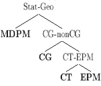
Figure 1. The binary decision tree
functionclassify, which is defined as follows:
classif y(X) =argmin{ωi}d(X) (1)
where d(X) =
q
(X−X(i))0
L∗(L∗0
SWL∗)−1L∗0(X−X(i)), SW =
PC
i=1Si,Si= P
X∈ωi(X−X(i))(X−X(i))0 andX(i)= 1
ni P
X∈ωiX.
IV. EXPERIMENT
We choose a LDA method as a selector based on one snapshot in order to provide an accurate estimation of the MS for location services. We extract 5 factors from each snapshot, which is described in section III. We have proposed several approaches to provide the estimation of the location of the MS for applications in our previous research work. We name these approaches as CG, CT, EPM and MDPM. Then we build up a database include the extracted factors from a snapshot and the results with four proposed algorithms.
For each snapshot, we classify it into one of algorithms classes based on its error, which is a criteria between the estimation of the location and the actual location of the MS. For example, if the result of MDPM algorithm reaches a minimum error within these algorithms, we classify these factors extracted from this snapshot into the MDPM class. And so on the other algorithms. Then we classify all these snapshots into one of these four algorithms classes based on our previous calculations. Then we have derived a new data source from our database of the extracted factors. We train the parameter of the LDA selector based on this new data source.
With the technical support of two mobile operators in Hong Kong, we have conducted an intensive field test in many regions in Hong Kong in order to validate our method. We choose total 116,284 sets snapshots to test our LDA selector.
Then the selector based on the information of snapshot is actual a C classes discriminant problem, where C
is four in our actual applications. We have discussed LDA method in C classes discriminant, which is just an extension of two classes discriminant. We need to find out three discriminant functions in order to distinguish these four classes. Namely, we need to provide three projection directions to classify these classes data.
Our research group has presented four algorithms for providing mobile location services within a cellular radio network: CG, CT, EPM and MDPM. And these four methods can be divided into two classes: the statistical model approaches and the geometric model approaches. MDPM is a statistical model approach. While CG, CT and EPM are all geometric methods to provide the mobile station location. The CG approach is a weighted mean of the locations of the BSs, thus it has the convex hull problem and CT and EPM have no this restraint. Then we can separate the geometric algorithms into two classes based on the restraint of convex hull problem. The EPM is an improvement algorithm of the CT algorithm. And EPM can always provide a solution while CT does not. So we also can separate the CT algorithm and EPM algorithm.
Then we can build up a three level binary decision tree to classify the snapshot into one of the four algo-rithms based on the above analysis. The decision can be illustrated in Figure. 1. Following our research thread, we set these three discriminant steps: statistical model and geometric model, CG and non CG methods and CT and EPM algorithm. We change aC classes discriminant problem into a(C−1)two classes discriminant problems in order to look insight into the character of our selector. We can clearly describe our selector in a three-level binary tree. It is a three levels binary tree, the nodes are these four algorithms. We distinguish the statistical model and geometric models in the first level, then classify the CG approach and non-CG approach in the second level within geometric model, then we discriminate the CT algorithm and EPM algorithm in the rest data in third level of this binary decision tree.
We use a table to show the results of our selector. And we choose the success ratio as a criterion to test our selector.success ratio= (1−error ratio)×100%, whereerror ratio= Error NumberTotal Number×100%. TableIare shown that the effect of these three discriminant functions. We have a good performance selector method with LDA inI. The success ratio of first level (Stat-Geo) is 85.22%. And the success ratio of second level (CG-nonCG) is 88.45% and the third level (CT-EPM) is 88.89%. As we can see, the success ratio becomes higher when in the deeper level of the binary tree (88.89% > 88.45% > 85.22%).
Discriminant Total Number Error Number success ratio %
Stat-Geo 116284 17186 85.22%
CG-nonCG 64989 7505 88.45 %
CT-EPM 38258 4252 88.89%
TABLE I. DISCRIMINANTRESULTS
Model Average Error Standard Deviation Imp.% sample number success ratio %
CG 482.99m 781.62 44.58% 116284 93.22%
CT 470.20m 904.24 43.08% 116284 78.58 %
EPM 359.47m 518.00 25.54% 116284 79.13%
MDPM with BE 324.22m 362.38% 17.44 116284 99.07%
Selector 267.66m 360.07 0% 116284 99.39%
TABLE II.
SELECTORRESULT: CG, CT, EPMANDMDPM
V. CONCLUSIONS ANDFUTUREWORK
We have presented a selector method with the LDA among some algorithms in this paper. The idea of selector is to find out a rule based on one snapshot to choose a “best” algorithm to provide an accurate estimation. The LDA is a statistical approach based on the variance analysis. The original idea of the LDA is attribute to R.A. Fisher, a great statistician, who presented a result known as Fisher’s Linear Discriminant in 1936. The LDA can be used to separate different classes data using projections, on the other hand, it also can be used to perform dimensionality reduction.
We have presented four algorithms in our previous work, denoted as CG, CT, EPM and MDPM. We are required to form a formula based on one snapshot in-formation to classify the data we have into one of these four algorithms. It is a4 classes discriminant problem of the LDA. We need to build up at most three discriminant functions in order to separate these four classes. Based on our research thread, CG, CT and EPM are all geometric algorithms. CG is a weighted mean of the locations of the BSs from which the MS receives signal strength, so CG is always inside a convex hull formed by these locations of BSs. CT is an algorithm which uses three BSs to provide the location of the MS. The CT estimation is a intersection of three circles formed by the locations of these three BSs and their received signal strengths. The CT algorithm has overcome the defect of the CG algorithm, which has a convex hull problem, but CT can not always provide a solution, since these three circles can not guarantee a intersection. In view of this, we proposed EPM algorithm to overcome the CT algorithm. EPM is derived from the CT algorithm, which is also using three BSs and their corresponding signal strengths to provide a solution. EPM extends the solution filed of the CT algorithm, then EPM can provide a feasible solution when the CT algorithm has no solution. If the CT algorithm has a solution, it is the same with the one of EPM. While MDPM is a statistical method to provide the location of the MS. First, we use some training data to build up a signal propagation
model, then provide a Bayes estimation based on this signal propagation model in test phrase.
Based on the above analysis, we change the C classes LDA problem into “C−1” two classes LDA problem, and then build up an at most C−1 steps decision tree to classify one snapshot into a class. It can improve the success ratio with this decision tree since it considers the properties of these algorithms. In our application, We build up a three-level binary tree for our selector. The first level includes two nodes, one is the geometric method, the other is the statistical approach (MDPM). If we can classify a snapshot into geometric method, we are required to have another discriminant. The second level of our binary tree has two nodes, one is the CG algorithm, the other is non-CG algorithm, since the CG estimation is always inside a convex hull, CT and EPM all have no convex hull problem. And the third level is a discriminant between CT and EPM. Each snapshot can be classified into an algorithm class at most three discriminants.
Our selector method is a try to provide a general solution for location services with different terrains and environments. Results have shown that the LDA selector is useful and outperforms other existing algorithms. Al-though our selector method is useful, it has two defects: One defect is that we need to build up a decision tree and then use a two-class LDA method to classify the snapshot in order to improve the success ratio. It is a semi-automatic selector since we need to build up a decision tree first, which depends on the properties of our algo-rithms. We are required to develop an automatic selector, which depends on the information of the snapshot and is independent with our algorithms. The other defect is that we use all the data to train the our selector, and then test it with the same data. It is admitted for academic research, but is unreasonable for application.
to abstract more features from a snapshot information. The more features of a snapshot we have, the easier we can classify it. The other is to try another statistical method or AI algorithm as a selector. LDA is one method to classify different classes data, other methods, such as SVM (Support Vector Machine), Bayes’s discrimi-nant, ANN(Artificial neural network) and KNN (k-nearest neighbor), can be chosen as a selector to provide an accurate estimation within a cellular radio network.
VI. RELATEDWORK
For the completeness of this paper, we list here the main ideas and approaches for each of the location estimation algorithm used for this investigation. Please refer to the following publications [7]–[10], [16] for the details.
Previously, our group has proposed two general al-gorithms for location estimation, namely, the Center of Gravity (CG) algorithm and the Circular Trilateration (CT) algorithm [7], [8]. Both CG and CT are making use of the RSS for estimating the position of a MS. They assumed the relationship between the MS-BS distance (d) and the RSS (s) iss∝d−2 based on theInverse Square Law[21]. However, due to the interference and distortion by buildings, this relationship is remodeled intos∝d−α, whereαis a variable relating to the environment.
A. Center of Gravity (CG) The CG approach is defined as:
x=x1s−1α+x2s2−α+x3s−3α+...+xns−nα s−α
1 +s−2α+s3−α+...+s−nα y= y1s−1α+y2s2−α+y3s−3α+...+yns−nα
s−1α+s−2α+s−3α+...+s−nα
(1)
where (x, y) is the estimated location of the MS. (x1, y1),(x2, y2), ...,(xn, yn) are the locations of n re-ceiving BSs.s1, s2, ..., snare the corresponding RSS from each BS [7].
Although the CG approach has proven its outstanding performance in metropolitan area, it can only estimate a mobile device inside the convex hull of the BSs involved, since the CG estimation is a weighted mean of the locations of the BSs involved.
B. Circular Trilateration (CT)
The basic idea of the CT algorithm is to construct 3 circles from the RSS of the corresponding three BSs. Given the locations of the three BSs and the mapping between the RSS and the MS-BS distance, the intersection of these three circles is the estimated location of the MS. Similar to CG, CT models the relationship between the MS-BS distance (d) and the RSS (s) asd∝(N+s)−α, whereN is a normalization constant. By making use of this relationship, we can construct three circles as follows,
(x−x1)2+ (y−y1)2= (sk1α)2 (x−x2)2+ (y−y2)2= (sk2α)
2
(x−x3)2+ (y−y3)2= (sk3α)2
(2)
where, s1, s2 ands3 are the RSSs from three receiving
BSs with their geographic locations as (x1, y1), (x2, y2)
and (x3, y3) respectively and k be a common scaling
factor. The location of the MS is then estimated as the intersection point of these three circles [8].
Although CT does not has the convex hull problem, it does not always provide an estimation. This is because the intersection may not always exist due to signal fading and signal fluctuation. Moreover, both CG and CT do not take the transmission direction of the BS into consideration, which is not realistic. Thus, we have designed a more realistic model, the Ellipse Propagation Model (EPM), which is an improvement of the CT algorithm.
C. The Ellipse Propagation Model
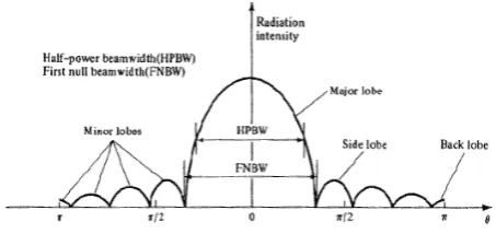
Figure 2. The directional transmission property
From our observations, we have found that BSs have directional transmission properties. The antenna transmits the signal in some specific directions. That is, the antenna transmits the largest power in one direction, while trans-mits small or none power in other directions. We can plot the signal strength with the same radius around an antenna as in Figure 2. As shown inFigure 2, the curve of the signal strength for a directional antenna is not a circle.
Thus, we assume that the contour line of the signal strength form an ellipse instead of a circle based on our studies. Furthermore, EPM adopts a different relationship between the MS-BS distance and the RSS. We can use the following mathematical formula to depict EPM.
d=k(s0/s)1/α 1−e
1−ecos(θ) (3) where
dis the distance between the MS and the BS; kis the proportion constant;
s0 is the transmitting power of the BS;
sis the signal power received;
eis the eccentricity of the ellipse, it describes the figure of the contour line;
θ is the deviation between the ellipse principal axis and the line of the MS-BS;
α is called the path loss exponent.
MS
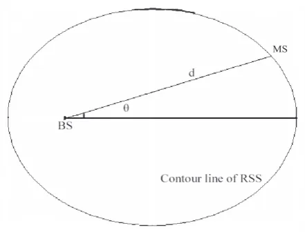
Figure 3. The Ellipse Propagation Model(EPM)
strength is an ellipse [9]. The Ellipse Propagation Model (EPM) can be illustrated in Figure 3.
EPM has four parameters:k,α,eandθ. We consider the parameters ofkandαas the region parameter, and the parametereis used to describe the figure of ellipse, while the deviation θ is a parameter for each MS. We use the field test data to estimate the values of these parameters, then translate the received signal strength (RSS) into a two-point distance.
We further combine this Ellipse Propagation Model (EPM) with the Geometric Algorithm, and with its en-hanced algorithm, the Iterative Algorithm, to provide a location of the MS in [9], [10]. The Ellipse Propaga-tion Model (EPM) considers the direcPropaga-tional transmission property of the antenna and assumes that the contour line of the signal strength for one antenna as an ellipse which the BS is at one of the focuses. On the other hand, the Geometric Algorithm derives from the CT algorithm to compensate its defect of not able to provide an estimation every time. We later on further propose the Iterative Algorithm to improve the Geometric Algorithm by choosing the convergence point as the location of the MS for estimation. Details of the Geometric Algorithm and the Iterative Algorithm with the EPM model are presented in the following sections.
1) The Geometric Algorithm under EPM: The Geo-metric Algorithm is used to provide an estimation of the location of the MS. We choose the value of deviation between the ellipse principal axis and the line of the BS and the center (or the weighted center) of the locations of the BSs as an estimation of θ, which is the deviation between the ellipse principal axis and the line of the MS and the BS. So EPM using the Geometric Algorithm exactly has three parameters:k, αande.
Suppose a MS receives RSSs,s1,s2,s3from three BSs
with locations,(x1, y1),(x2, y2),(x3, y3)respectively. In
addition, the distances between the MS and the BSs are denoted by d(s1),d(s2),d(s3), sometimes, and they are
simply denoted by d1,d2 and d3. Thus, by the formula
of the two points distance in a 2-D Euclidian space, we
can form these three circles formulas as follows,
(x−x1)2+ (y−y1)2=d21 (x−x2)2+ (y−y2)2=d22 (x−x3)2+ (y−y3)2=d23
(4)
Basically, the geometric interpretation of this equation group means three circles in a 2-D space, and the solution is the intersection point of these three circles. However, if an intersection point does not exist, we may not be able to provide an estimation for the location of the MS. In order to solve this problem, the Geometric Algorithm does not solve this equation group directly. Instead, the Geometric Algorithm derives another three equation groups from this equation group (4). As each new equation group can provide a solution, thus, we will have three solutions. The estimation of the location of the MS will then be the center of these three solutions [9]. Thus, the algorithm always provides a solution.
The solution of one equation group from (4) is: ½
x= (2m(y3−y1)−2n(y2−y1))/|A|
y= (−2m(x3−x1) + 2n(x2−x1))/|A| (5)
where
|A|= 4[(x2−x1)(y3−y1)−(x3−x1)(y2−y1)]; m= [d2
1−(x21+y12)]−[d22−(x22+y22)]; n= [d2
1−(x21+y12)]−[d23−(x23+y32)]; (x1, y1),(x2, y2),(x3, y3)are the BSs locations.
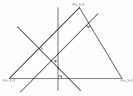
The Geometric Algorithm uses three distances between the MS location and the locations of BSs to estimate the MS location. The Geometric Algorithm used three lines formed by these three receiving BSs to provide the estimation. In this case, we always obtain a solution if these three receiving BSs are not in a straight line. We can form a straight line by subtracting one circle with another circle. Therefore, we can obtain three combina-tions of these three straight lines. These three straight lines intersect with each other if and only if they are not parallel. Thus, we have three intersections and then we can estimate the position of the MS as the center of these three intersections. Figure 4 demonstrates the Geometric Algorithm graphically. From Figure 4, these three vertexes marked by (x1, y1), (x2, y2) and (x3, y3)
are the locations of these three receiving BSs while the ”cross” point is the estimated location of the MS by the Geometric Algorithm, which is the center of these three intersections.
Figure 4. The Geometric Interpretation
have better accuracy than the Geometric Algorithm by eliminating these errors.
Suppose a MS received RSSs, s1, s2, s3 from three
BSs with the locations, l1(α1, β1),l2(α2, β2),l3(α3, β3)
and the output powers,o1,o2,o3respectively. In addition,
the distances between the MS and the BSs are denoted byd1,d2,d3.
From the Iterative Algorithm, we have, ½
x=f(x, y;s1, s2, s3;l1, l2, l3)
y=g(x, y;s1, s2, s3;l1, l2, l3) (6)
Then, we depict the Iterative Algorithm by using the Geometric Algorithm structure based on EPM. We can get the following formulas in [10]:
½
x= (2m(β3−β1)−2n(β2−β1))/|A|
y= (−2m(α3−α1) + 2n(α2−α1))/|A|
where
|A|= 4[(α2−α1)(β3−β1)−(α3−α1)(β2−β1)];
m= (α2
2+β22)−(α21+β12) + (d21−d22);
n= (α2
3+β32)−(α21+β12) + (d21−d23);
d1=k(o1/s1)1/α(1−e1)/(1−e1cos(θ1));
d2=k(o2/s2)1/α(1−e2)/(1−e2cos(θ2));
d3=k(o3/s3)1/α(1−e3)/(1−e3cos(θ3));
α is the path loss exponent; kis the proportion constant;
e1,e2 and e3 are the eccentricities of the ellipses;
θ1,θ2and θ3 depend onxand y.
D. The Modified Directional Propagation Model While CG, CT and EPM are all geometric approaches to provide the estimation of the location of the MS, the Modified Directional Propagation Model (MDPM) is a statistical method to provide an estimation of the location of the MS. Based on our studies, the probabilis-tic approach has better performance than the geometric approach in terms of accuracy.
The mean of the RSS is defined as:
µ(p, d, h, e, δ, β) =p+β0+β1cos(δ) +β2log(h)+
(β3+β4e+β5log(h))ln(d) +β6h
(7) where µ(p, d, h, e, δ, β) is the mean received signal strength in decibels; p is the transmitted signal strength in decibels; d is the distance in meter between the MS and the BS; e is the environment index and δ is the deviation between the direction of transmission and the direction of the receiver as measured from the transmitter, the values ofδare clearly between zero and 180 degrees. β= (β0, β1, β2, β3, β4, β5, β6)T are the parameters of the
signal propagation model, α = β3+β4e+β5log(h) is
called the path loss exponent, andhis the height in meter of the antenna.
We use the iterative method to provide the estimation of the model parameter, then provide a Bayes Estimate as the estimation of the location of the MS [16].
ACKNOWLEDGEMENT
The authors would like to thank the reviewers and the Editor-in-Chief for their helpful instruction and valuable comments on how to improve this paper.
The work reported was supported in part by the Innova-tion and Technology Fund (ITS/02/22) of the InnovaInnova-tion and Technology Commission and also supported by the Central Allocation Grant (HKBU 1/05C) of the Research Grant Council of University Grant Council of the Hong Kong SAR Government.
Some of this work was presented at the ARES 2006 conference. And a shorter version of this paper is pub-lished in the proceedings of ARES 2006 [22].
REFERENCES
[1] Peter H. Dana, Global Positioning
Sys-tem Overview, The University of Texas, http://www.colorado.Edu/geography/gcraft/notes/gps /gps.html.
[2] Richard Walter Klukas, Gerard Lachapelle, and Michel Fattouche, Cellular Telephone Positioning Using GPS Time Synchronization, The University of Calgary, http://www.geomatics.ucalgary.ca/Papers/Thesis /GL/97.20114.RKlukas.pdf.
[3] Federal Communications Commission, “Revision of the commission’s rules to ensure compatibility with enhanced 911 emergency calling systems,” Report and Order and Further Notice of Proposed Rulemaking, Tech. Rep. CC Docket No. 94-102, July 1996.
[4] Kaveh Pahlavan, Prashant Krishnamurthy, Principles of Wireless Networks a Unified Approach. Pearson Edu-cation, Inc., 2002.
[5] Svein Yngvar Willassen, Steinar Andresen, A Method of implementing Mobile Station Location in GSM, Norwegian University of Science and Technology, http://www.willassen.no/msl/bakgrunn.html.
[7] Joseph Kee-Yin Ng, Stephen Ka Chun Chan, and Shibin Song, “A Study on the Sensitivity of the Cen-ter of Gravity Algorithm for Location Estimation,” Hong Kong Baptist University, Tech. Rep., May 2003, http://www.comp.hkbu.edu.hk/tech-report/tr03014f.pdf. [8] Kenny K.H. Kan, Stephen K,C. Chan, and Joseph K.
Ng, “A Dual-Channel Location Estimation System for providing Location Services based on the GPS and GSM Networks,” inProceedings of The 17th International Con-ference on Advanced Information Networking and Appli-cations(AINA 2003), Xi’an, China, March 2003, pp. 7–12. [9] Junyang Zhou, Kenneth Man-Kin Chu, Joseph Kee-Yin Ng, “Providing Location Services within a Radio Cellular Network using Ellipse Propagation Model,” inProceedings of the 19th International Conference on Advanced Infor-mation Networking and Applications (AINA 2005), Taipei, Taiwan, March 28-30 2005, pp. 559–564.
[10] Junyang Zhou, Kenneth Man-Kin Chu, Joseph Kee-Yin Ng, “An Improved Ellipse Propagation Model for Loca-tion EstimaLoca-tion in facilitating Ubiquitous Computing,” in Proceedings of the 11th IEEE International Conference on Embedded and Real-Time Computing Systems and Appli-cations (RTCSA 2005), Hong Kong, Aug. 17-19 2005, pp. 463–466.
[11] Teemu Roos, Petri Myllym¨aki, Herry Tirri, “A Statistical Modeling Approach to Location Estimation,”IEEE Trans-actions on Mobile Computing, vol. 1, no. 1, pp. 59–69, January-March 2002.
[12] M. McGuire, K. Plataniotis, A. Venetsanopoulos, “Esti-mating Position of Mobile Terminals with Survey Data,” EURASIP Journal on Applied Signal Processing, vol. 2002, no. 1, pp. 58–66, January 2002.
[13] M. McGuire, K. Plataniotis, A. Venetsanopoulos, “Esti-mating Position of Mobile Terminal from Path Loss Mea-surements with Survey Data,” Wireless Communications and Mobile Computing, vol. 3, no. 1, pp. 51–62, February 2003.
[14] Kenneth M. Chu, Karl R.P.H. Leung, Joseph K. Ng, and Chun H. Li, “Locating Mobile Stations with Statistical Directional Propagation Model,” inProceedings of the 18th International Conference on Advanced Information Net-working and Applications (AINA 2004), Fukuoka, Japan, March 2004, pp. 230–235.
[15] Kenneth M. Chu, and Joseph K. Ng, “Estimat-ing Propagation Parameters us“Estimat-ing a Modified EM Algorithm for Mobile Location Estimation,” Hong Kong Baptist University, Tech. Rep., Nov. 2004, http://www.comp.hkbu.edu.hk/tech-report/tr04007f.pdf. [16] Junyang Zhou, Kenneth Man-Kin Chu, Joseph
Kee-Yin Ng, A New Approach to Mobile Location Es-timation within a Radio Cellular Network, submit to IEEE Transactions on Mobile Computing, avail-able at URL:http://www.comp.hkbu.edu.hk/ jyzhou/paper /MJPZhou2005.pdf.
[17] David Mount, “Computational Geometry,” Dept. of Computer Science, University of Maryland, College Park, MD, 20742, pp. 13–14, 2002, lecture Notes for the course CMSC 754. [Online]. Available: http://www.cs.umd.edu/ mount/754/Lects/754lects.pdf [18] Alvin C. Rencher, Multivariate Statistical Inference and
Applications. John Wiley & Sons, Inc., 1998.
[19] R.A.Fisher, “The use of multiple measurements in taxo-nomic problems,”Annals of Eugenics, vol. VII, no. II, pp. 179–188, 1936.
[20] Richard O. Duda, Peter E. Hart, David G. Stork, Pattern Classification, Second Edition. Wiley, 2000.
[21] “Inverse square law,” http://hyperphysics.phy-astr.gsu.edu/hbase/forces/isq.html.
[22] Junyang Zhou, Joseph Kee-Yin Ng, “A Selector Method for Providing Mobile Location Estimation Services within
a Radio Cellular Network,” in Proceedings The First International Conference on Availability, Reliability and Security (ARES 2006), Vienna, Austria, April 20-22 2006, pp. 82–89.
Junyang Zhou received a B.Sc. in Applied Mathematics, a M.Sc. in Probability and Mathematic Statistics from Sun Yat-sen University in 2000 and 2003, respectively. He is currently a Ph.D candidate in Department of Computer Science at Hong Kong Baptist University. His current research interests include: Mobile and Location-aware Computing, Ubiquitous/Pervasive Computing, Real-Time Network and Bayesian Network.
Joseph Kee-Yin Ng received a B.Sc. in Mathematics and Computer Science, a M.Sc. in Computer Science, and a Ph.D. in Computer Science from the University of Illinois at Urbana-Champaign in the years 1986, 1988, and 1993, respectively. Prof. Ng is currently a professor in the Department of Computer Science at Hong Kong Baptist University.
His current research interests include Real-Time Networks, Multimedia Communications, Ubiquitous/Pervasive Computing, Mobile and Location- aware Computing, Performance Evalua-tion, Parallel and Distributed Computing. Prof. Ng is the Tech-nical Program Chair for TENCON 2006, General Co-Chair for The 11th International Conference on Embedded and Real-Time Computing Systems and Applications (RTCSA 2005), Program Vice Chair for The 11th International Conference on Parallel and Distributed Systems (ICPADS 2005), Program Area-Chair for The 18th & 19th International Conference on Advanced Information Networking and Applications (AINA 2004 & AINA 2005) and he had served as the General Co-Chair for The Inter-national Computer Congress 1999 & 2001 (ICC’99 & ICC’01), the Program Co-Chair for The Sixth International Conference on Real-Time Computing Systems and Applications (RTCSA’99) and the General Co-Chair for The 1999 and 2001 International Computer Science Conference (ICSC’99 & ICSC’01).
Prof. Ng is a member of the Editorial Board of Journal of Per-vasive Computing and Communications, Journal of Ubiquitous Computing and Intelligence, Journal of Embedded Computing, and Journal of Microprocessors and Microsystems. He is the Associate Editor of Real- Time Systems Journal and Journal of Mobile Multimedia. He is also a guest editor of International Journal of Wireless and Mobile Computing for a special issue on Applications, Services, and Infrastructures for Wireless and Mobile Computing.